HAL Id: hal-00641722
https://hal.archives-ouvertes.fr/hal-00641722v2
Submitted on 18 Nov 2011HAL is a multi-disciplinary open access
archive for the deposit and dissemination of sci-entific research documents, whether they are pub-lished or not. The documents may come from teaching and research institutions in France or
L’archive ouverte pluridisciplinaire HAL, est destinée au dépôt et à la diffusion de documents scientifiques de niveau recherche, publiés ou non, émanant des établissements d’enseignement et de recherche français ou étrangers, des laboratoires
RAPID applied to the SIM-France model
Cédric David, Florence Habets, David Maidment, Zong-Liang Yang
To cite this version:
Cédric David, Florence Habets, David Maidment, Zong-Liang Yang. RAPID applied to the SIM-France model. Hydrological Processes, Wiley, 2011, 25 (22), pp.3412-3425. �10.1002/hyp.8070�. �hal-00641722v2�
RAPID applied to the SIM-France model
1 2
Cédric H. David1,2,3 ([email protected]), Florence Habets4 3
([email protected]), David R. Maidment2 ([email protected]) 4
and Zong-Liang Yang3 ([email protected]) 5
6
1. Centre de Géosciences, Mines Paristech, Fontainebleau, France 7
2. Center for Research in Water Resources, University of Texas at Austin, Austin, Texas, 8
USA. 9
3. Department of Geological Sciences, Jackson School of Geosciences, University of 10
Texas at Austin, Austin, Texas, USA. 11
4. UMR-7619 Sisyphe [CNRS, UPMC, Mines-Paristech], Paris, France. 12 13 Corresponding author 14 Cédric H. David 15
Department of Geological Sciences, Jackson School of Geosciences 16
The University of Texas at Austin 17 1 University Station C1160 18 Austin, TX 78712 19 [email protected] 20 +1 512 299 7191 (cell) 21 +1 512 471 5355 (office) 22
(No fax number available) 23
Abstract
24
SIM-France is a large connected atmosphere/land surface/river/groundwater modeling 25
system that simulates the water cycle throughout metropolitan France. The work 26
presented in this study investigates the replacement of the river routing scheme in SIM-27
France by a river network model called RAPID to enhance the capacity to relate 28
simulated flows to river gages and to take advantage of the automated parameter 29
estimation procedure of RAPID. RAPID was run with SIM-France over a ten-year 30
period and results compared with those of the previous river routing scheme. We found 31
that while the formulation of RAPID enhanced the functionality of SIM-France, the flow 32
simulations are comparable in accuracy to those previously obtained by SIM-France. 33
Sub-basin optimization of RAPID parameters was found to increase model efficiency. A 34
single criterion for quantifying the quality of river flow simulations using several river 35
gages globally in a river network is developed that normalizes the square error of 36
modeled flow to allow equal treatment of all gaging stations regardless of the magnitude 37
of flow. The use of this criterion as the cost function for parameter estimation in RAPID 38
allows better results than by increasing the degree of spatial variability in optimization of 39
model parameters. Likewise, increased spatial variability of RAPID parameters through 40
accounting for topography is shown to enhance model performance. 41
42
Keywords stream flow, river network, network matrix, parameters, estimation, dam,
quad-43
tree
44 45
1. Introduction
46
In the past two decades, several large scale river routing schemes have been used along 47
with land surface models for hydrologic modeling. Among the most notable applications 48
of large scale river routing are TRIP [Total Runoff Integrating Pathways, Ngo-Duc, et al., 49
2007; Oki and Sud, 1998], RiTHM [River-Transfer Hydrological Model, Ducharne, et 50
al., 2003], the routing model of Lohmann et al. [Lohmann, et al., 1996; 1998a; 1998b;
51
1998c; 2004; Maurer, et al., 2001], that of Wetzel [Abdulla, et al., 1996; Nijssen, et al., 52
1997; Wetzel, 1994], and that of Olivera et al. [2000]. These approaches have been used 53
along with land surface parameterization schemes to calculate river flow from runoff at 54
the regional, continental and the global scale. MODCOU [Modèle Couplé, Ledoux, et 55
al., 1989] is another model with routing capabilities that differs from the previously cited
56
models in that it has two separate networks of grid cells for horizontal routing of water on 57
the land surface: one for overland routing and one for routing within the river system. 58
MODCOU simulates flows throughout Metropolitan France (mainland France and 59
Corsica) as part of the SIM-France modeling framework [Habets, et al., 2008]. 60
SIM-France (SAFRAN-ISBA-MODCOU-France) is a large connected atmosphere, land 61
surface, river and groundwater model (see Figure 1) that involves coupling the national-62
scale atmospheric analysis system SAFRAN [Système d'Analyse Fournissant des 63
Renseignements Atmosphériques à la Neige, Durand, et al., 1993; Quintana-Seguỉ, et al., 64
2008], with the ISBA land surface model [Interactions Soil- Biosphere-Atmosphere, 65
Boone, et al., 1999; Noilhan and Planton, 1989], and with the MODCOU
66
hydrogeological model [Ledoux, et al., 1989]. ISBA computes the vertical water and 67
energy balance between the land surface and the atmosphere. The improved physics of 68
the land surface parameterization of ISBA that consist of an exponential profile for soil 69
hydraulic conductivity developed in Decharme et al. [2006] with calibration of soil 70
hydraulic conductivity and subgrid runoff over France by Quintana-Seguí et al. [2009] 71
are used in this study. Surface runoff and deep-soil drainage are computed by ISBA and 72
transferred to MODCOU which computes the horizontal flow routing on the land surface, 73
in rivers and in aquifers. Aquifers in MODCOU are modeled within the two main river 74
basins of France, the Seine and the Rhône, which together represent 30% of the land area 75
of France. 76
MODCOU handles the calculations of flow and volume of water within the river network 77
of SIM-France. This river network is made up of grid cells divided into a quad-tree 78
pattern and the calculations of MODCOU are made for groups of quad-tree cells; not for 79
each quad-tree cell separately. Using groups of cells for calculations is advantageous for 80
reducing computational costs but it limits the modularity of MODCOU. In particular, the 81
location and number of gaging stations are difficult to modify. 82
The work presented herein investigates the impact of replacing the routing module used 83
in MODCOU by a river network model called RAPID [Routing Application for Parallel 84
ComputatIon of Discharge, David, et al., 2011]. RAPID uses a matrix-based version of 85
the Muskingum method to calculate flow and volume of water for each reach of a river 86
network separately and has an automated parameter estimation procedure. RAPID 87
therefore allows greater flexibility than the routing module in MODCOU with regards to 88
changing the locations of computations in an existing domain or to running SIM on a new 89
domain. RAPID was previously applied to a GIS vector river network [David, et al., 90
2011], and the present study shows how it can also be applied to a quad-tree gridded river 91
network. In addition, RAPID is advantageous because of its ability to run in a parallel 92
computing environment and its fine time step allowing potential comparison with river 93
flow observations at high temporal resolution. Finally, replacing the routing module of 94
MODCOU by RAPID has already allowed computing river flow height and helping 95
quantify river/aquifer interactions at the regional scale [Saleh, et al., 2010; 2011]. 96
In this paper, the original river routing of MODCOU as well as that of RAPID are briefly 97
presented followed by a ten-year application (1995-2005) of SIM-France comparing the 98
two river routing applications for different sets of parameters used in RAPID. 99
2. Modeling framework
101
2.1. River modeling in SIM-France
102
The computational domain of SIM-France includes all of Metropolitan France, including 103
Corsica. Parts of Spain, Switzerland, Germany and Belgium are also included where 104
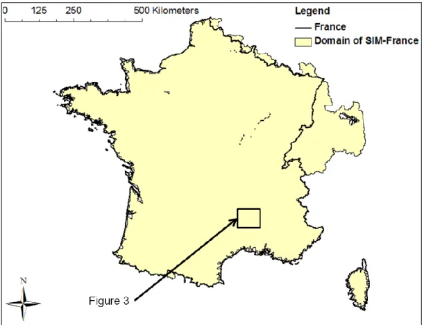
their drainage area flows through France, as shown in Figure 2. The total surface area of 105
the computational domain is 610,000 km2. 106
Surface routing and river routing in SIM-France are done by MODCOU [Ledoux, et al., 107
1989]. The surface and river networks of SIM-France and their connectivity were created 108
using a routine called HydroDem [Leblois and Sauquet, 2000] and consist of 193,861 109
surface cells and 24,264 river cells, each river cell being a particular surface cell. The 110
surface area covered by the river cells is 65,000 km2. The surface network uses a quad-111
tree structure with cell sizes of 1 km, 2 km, 4 km and 8 km. The river network has cell 112
sizes of 1 km and 2 km. The smaller quad-tree cells are used at the conference of 113
branches of the river network for better representation of the network connectivity and at 114
basin boundaries for more accurate basin surface area. 115
The connectivity between river cells is given by a table that provides for each 116
downstream river cell up to three upstream river cells. There are no loops or divergences 117
in the river network of SIM-France. The connectivity between catchments and rivers is 118
given by a table that provides for each surface cell a unique downstream cell where its 119
runoff enters the river. 120
For both surface and river routing, the calculations of flow and volume of water within 121
MODCOU are carried out using groups of cells as computing elements, therefore 122
minimizing the amount of calculations compared to computing for all cells separately. 123
These groups of cells – or isochrone zones – are based on the notion of isochronism 124
developed by Leblanc and Villeneuve [1978]. An isochrone is a line representing a 125
constant time of travel to a reference point downstream. An isochrone zone is the area 126
between two successive isochrones. This zone is represented by a set of cells which are a 127
single computational unit in MODCOU. Both the land surface isochrones and river 128
isochrones of MODCOU have three-hour time intervals, which means that the time of 129
travel between the upstream-most and the downstream-most cell in a given isochrone 130
zone is approximately three hours. All the isochrones of a given network are determined 131
using the travel time between connected cells which is estimated based on topography 132
and on the geometry of the quad-tree mesh. For surface cells and river cells, the travel 133
time i j, between two consecutive cells i and j is calculated using the distance
134
,
i j
d between the two cells and the slope si j, , as shown in Equation (1):
135 136 , , , i j i j i j d s (1) 137 138
where is the inverse of a velocity. In the current version of SIM-France, a unique 139
value of is calibrated for each major basin. 140
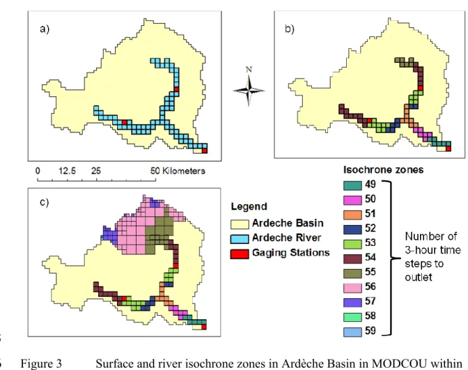
Figure 3 shows an example of the isochrone zones and connectivity between surface cells 141
and river cells in MODCOU for the Ardèche River Basin. Figure 3a) shows the Ardèche 142
River, its basin and three river gages. Figure 3b) shows the river isochrone zones of the 143
Ardèche River. Figure 3c) shows the surface isochrone zones corresponding to the 144
upstream-most river isochrone zone. Each surface cell belongs to a surface isochrone 145
zone, but only the isochrone zones corresponding to one river isochrone zone are shown 146
of Figure 3c) for clarity. The units used for isochrone zones are the number or 147
MODCOU 3-hour time steps to the outlet (here the Mediterranean). The quad-tree 148
structure of increasing resolution can be seen at the boundary of the basin in Figure 3c). 149
In MODCOU, the volume of water out
V that discharges across each isochrone line in a
150
computation time step is calculated differently for the surface network and for the river 151
network. For routing on the land surface, all the volume of water V available in the
152
isochrone zone is transferred to the downstream zone, as shown in Equation (2): 153 154 out V V (2) 155 156
For routing in the river network, out
V is proportional to the volume of water V available
157
within the isochrone zone as shown in Equation (3): 158 159 out V V (3) 160 161
where [0,1]is manually calibrated and usually set constant for large basins. Equation 162
(3) can be viewed as the linear reservoir equation associated with a first-order explicit 163
development of the continuity equation. The variation of volume related to lateral inflow 164
and groundwater inflow of water are added to the volume V before calculating Vout. In
165
SIM-France, has four possible values: 0.5, 0.7, 0.8 and 0.9 as shown in Figure 4. 166
Equation (3) is applied to isochrone zones. Hence, the volume of water within each 167
isochrone zone needs be partitioned among its several river cells before computation of 168
the river-aquifer exchanges. This interaction depends on the aquifer head, on the river 169
head – assumed constant – and on the volume of water in the river cell when the river 170
infiltrates water into the aquifer. The partitioning of water volume among all cells of an 171
isochrone zone is done using a weighted average of the total amount of water reflecting 172
the spatial distribution of lateral inflow in each isochrone zone. 173
This formulation has several inconsistencies, especially when the junction between two 174
streams lies in the interior of an isochrone zone. This can have a consequence in river-175
aquifer interactions, but also in the computation of river flow. Furthermore, using only 176
one set of isochrones in each basin can lead to two gages being located in one isochrone 177
zone (for example a zone containing a confluence with gaging stations on both sides), in 178
which case the flow computed by MODCOU has to match the flow at two different 179
gaging stations. In order to avoid such inconsistencies, MODCOU uses a unique set of 180
isochrone zones for each gage, such that each gage is the downstream-most river cell in 181
its isochrone zone. Therefore, several flow calculations can be performed for a given 182
cell, if the given cell belongs to several isochrone zones, which is inefficient and requires 183
time consuming processing work in case of change of number or locations or river gages. 184
The work done herein aims at simplifying the river modeling done within SIM-France 185
and to ensure evolution of the code as for instance the computation of river flow height 186
[Saleh, et al., 2010; 2011] and velocity. 187
2.2. RAPID
RAPID [David, et al., 2011] is a river network model that uses a matrix-based version of 189
the Muskingum routing scheme to calculate discharge simultaneously through a river 190
network. RAPID was first applied to the Guadalupe and San Antonio River Basins in 191
Texas using a vector-based river network extracted from a geographic information 192
system dataset called NHDPlus [USEPA and USGS, 2007]. The governing equation used 193
in RAPID is the following: 194
195
I C N Q 1
t t
C Q1 e
t C2
N Q
t Qe
t
C Q3
t (4) 196197
where t is time and tis the river routing time step. The bolded notation is used for
198
vectors and matrices. All matrices are square. Iis the identity matrix. Nis the river 199
network connectivity matrix which has a value of one in element N if reach j flows i j,
200
into reach i and zero elsewhere. C ,1 C and 2 C are parameter matrices which depend on 3 201
Muskingum k , x and time step t. Q
t is a vector of outflows from river reaches,202
andQe
t is a vector of lateral inflows to these reaches from land surface runoff or203
groundwater inflow. The number of river quad-tree cells – here 24,264 – is used for 204
dimension of all vectors and matrices, each element of the vectors corresponding to one 205
river cell. 206
Provided with a vector of lateral inflows Qe
t , RAPID calculates the flow and volume207
of water in all reaches of a river network, therefore allowing coupling of a river network 208
to most land surface models and groundwater models. A different value for the 209
parameters kand x of the Muskingum method can be assigned for each river quad-tree
cell, and RAPID uses two vectors k and xas input which are used to compute the values 211
of the matrices C ,1 C and 2 C . However, before routing with RAPID, horizontal surface 3
212
and subsurface routing is needed to transport runoff from a land surface cell to its 213
corresponding river cell. In the present study, this surface and subsurface routing is done 214
by MODCOU and RAPID replaces only the river modeling of MODCOU. 215
The connectivity information that already exists between the river cells in the SIM-216
France river network is used to create the network connectivity matrix Nneeded by 217
RAPID and described in David et al. [2011]. 218
RAPID uses an automated parameter estimation procedure which, given lateral inflow 219
e
Q everywhere in the river network, and gage measurements at some locations,
220
determines a best set of parameters based on a square error cost function. As in David et 221
al. [2011], the search for optimal vectors of parameters k and xis made by determining 222
two multiplying factors kand xsuch that:
223 224 0 [1, 24264] j k Lj , j x 0.1 j k x c (5) 225 226
where j is the index of a quad-tree river cell, kj
and
j
xare its Muskingum parameters,
227
j
L is the flow distance within a river cell and c01km h 10.28m s 1 is a reference
228
celerity for the flow wave. The parameterskj
and
j
x are the same developed in David et
229
al. [2011] and are referred to as parameters in the following. In this study, the size of 230
the side of each quad-tree river cell was used as an approximation of its flow distance. 231
The value of xis bounded by the interval [0,5]since the Muskingum method is stable
232
only for x[0.0, 0.5], as shown in Cunge [1969]. The two scalars kand xare
233
determined such that the corresponding vectors k and xminimize the value of an 234
optimization criteria, or cost function. At the end of the optimization procedure, one 235
couple
k, x
is determined for a given part of the network. The values of kand xcan 236be determined for the entire study domain, or for sub-basins. If a sub-basin is located 237
downstream of another sub-basin, observations at a gaging station are used to provide the 238
upstream flow. Therefore, the delineation of sub-basins has to be consistent with the 239
location of available gage measurements. 240
The optimization procedure uses a line-search algorithm called the Nelder-Mead method 241
[Nelder and Mead, 1965] to determine the two scalars kand x. 242
The use of RAPID within SIM-France allows for flow and volume calculation at each 243
river cell and RAPID allows for the ready inclusion of additional river gages to be used 244
for calibration. 245
3. Application of RAPID in France
247
3.1. Optimization of RAPID parameters
248
This section focuses on the optimization of RAPID parameters with various options used 249
for k and j x , for the optimization cost function and for the spatial variability of the j
250
optimization. Two formulations are applied for computing k and j x including one j
251
formulation taking topography into account, two cost functions are tested, and three 252
different domain decompositions are used for optimization of parameters. In order to 253
simplify the optimization procedure and to ensure its repeatability, the parameter 254
estimation of RAPID was run uncoupled from SIM-France. Lateral and groundwater 255
inflow to the river network were obtained from a simulation using the standard version of 256
SIM-France (without RAPID) augmented with improved physics of the land surface 257
parameterization of ISBA developed in Decharme et al. [2006] and calibrated over 258
France by Quintana-Seguí et al. [2009]. Daily gage measurements from the French 259
HYDRO database [SCHAPI, 2008] were used for the parameter estimation as well as for 260
comparison with daily-averaged flow calculations . 261
The period of interest of the present study is August 1st 1995 to July 31st 2005. However, 262
the parameter estimation was performed using five months of the first winter (November 263
1st 1995 to March 31st 1996). As part of the first year (1995-1996) was used for 264
calibration, separate statistical results are presented for 1995-1996 and 1995-2005. 265
RAPID is run using a 30-minute time step and forced with 3-hourly lateral inflow 266
volumes; daily averages of computed discharge are compared with daily observations at 267
gage locations. There are 907 stations within the river network of SIM-France but only 268
493 of these have daily measurements every day during the first year (August 1st 1995 to 269
July 31st 1996). Amongst the 493 available stations, the best 291 were utilized for 270
optimization of RAPID parameters. The criterion used for the selection of the 291 best 271
stations is a Nash efficiency [Nash and Sutcliffe, 1970] better than 0.5 in the existing 272
SIM-France model (without RAPID) over 1995-1996. This selection excludes the gages 273
that are affected either by dams or by water diversions, and thus avoids unrealistic model 274
parameters due to anthropogenic modifications of river flow. Therefore, the proposed 275
routing scheme is optimized at locations were the previous routing scheme already 276
performed well. 277
The optimization is first performed on all rivers of the domain, therefore obtaining unique 278
values of kand xfor all 24,264 river quad-tree cells. However, such an optimization
279
may not capture the variability between river basins and within sub-basins, due to the 280
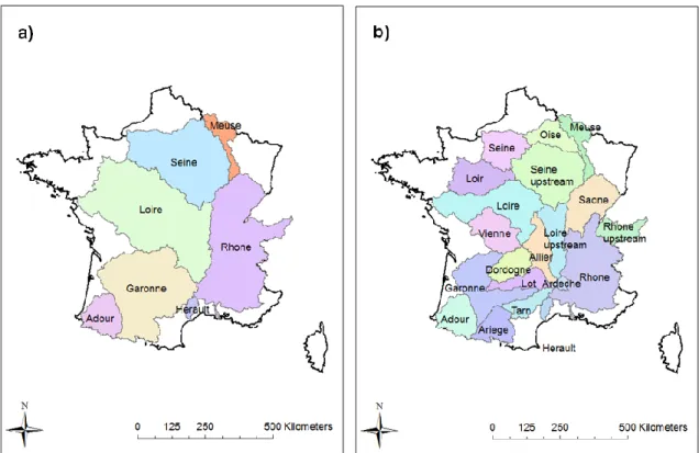
various slopes or soil types. Therefore, the optimization procedure was also run 281
independently within the seven main river basins of France shown in Figure 5a) and 282
within the twenty sub-basins shown in Figure 5b). 283
In order to limit the effect of the initial state of the system at the beginning of the 284
optimization procedure, the initial flows on 01 November 1995 were estimated using a 285
simple run of RAPID. This estimation was obtained through running the routing model 286
from 01 August to 31 October 1995 with uniform values of kand xover the study
287
domain and initial flows 3
0 m /sfor all river cells on 01 August 1995.
288
The results of a parameter estimation procedure depend slightly on the initial guess for 289
the parameters. Therefore, three different sets of initial guesses for kand x were used: 290
k, x
2,3 ,
k, x
4,1 or
k, x
1,1 . The numerical values of these three 291sets have no particular meaning and serve to start the optimization with a different initial 292
value for k and x. Each set of initial guesses leads to slightly different results for the 293
optimal kand x. Out of the three sets of optimal kand x that are determined for 294
each sub-basin, only the best is kept. This selection is based on the set of parameters that 295
leads to the smallest value of the optimization cost function. 296
Once the optimization procedure was completed, RAPID was run with SIM-France over 297
a 10-year period, from August 1995 to July 2005. This section focuses on the first year 298
while the next section studies the ten-year run. In order to compare the overall 299
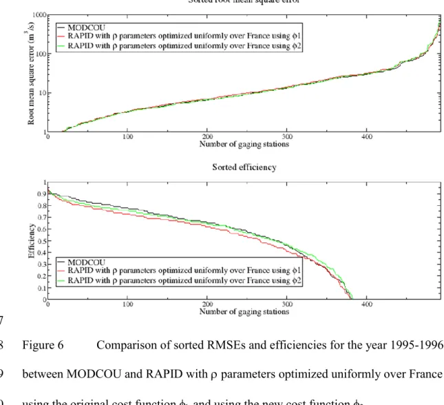
performance of both routing models on the river network, the Nash efficiency and the 300
root mean square error (RMSE) were calculated for each of the 493 gaging stations over 301
1995-1996. These criteria are sorted and comparisons between the computations of 302
MODCOU and those of RAPID are shown in Figure 6. The two graphs in Figure 6 do 303
not allow comparing both models at each gaging station since the criteria are sorted, but 304
they depict the overall relative performance of both models. Table 1 shows the average 305
Nash efficiencies and RMSEs obtained by the original version of SIM-France and with 306
RAPID using various optimization procedures. During 1995-1996, 382 stations have a 307
positive efficiency using the standard version of SIM-France. The averages presented in 308
Table 1 show the best 382 values for both efficiency and RMSE, but similar patterns are 309
found for all 493 values or the best 291 values. 310
In its original formulation, the criterion used in the optimization of RAPID is based on a 311
square error cost function 1. This function is the sum of the square errors between daily
measurements g
iQ t and daily-averaged Q t flow computations for several river i
313
gaging stations i and for everyday of a given period of time [ , ]t to f , as shown in
314 Equation (6). 315 316
2 291 1 1 , f o t t i g i i t t i Q t Q t f
k x (6) 317 318where the summation is made daily and at river cells with active gaging stations only. t o
319
and tfare respectively the first day and last day used for the calculation of 1.
320
[1, 291]
i is the index for gaging stations. The model parameter vectors k and x are
321
kept constant within the temporal interval [ ,t to f], and the cost function is calculated
322
several times with different sets of parameters during the optimization procedure. f is a 323
scalar that allows 1 to be of the order of magnitude of 101 which is helpful for automated 324
optimization procedures. One can notice that, in 1, a given fractional error (5% error
325
between modeled and measured flow for example) for two stations with different orders 326
of magnitude for river flow influences the cost function differently. A small fractional 327
error on a gaging station with a large flow penalizes the cost function more than the same 328
fractional error on a gaging station with small flow. The Nash efficiency Eis highly
329
influenced by the difference between the model computation and the mean average flow, 330
as shown in Equation (7): 331
2 2 1 f o f o t t g i i t t t t g g i i t t Q t Q t E Q t Q
(7) 333 334 where g iQ is the average daily flow observed at the gaging station i over a long
335
interval. Therefore, the use of 1 penalizes the Nash efficiency. In order to avoid that the
336
order of magnitude of flow at each gaging station influences their weight in the cost 337
function, a new cost function 2is created, as shown in Equation (8): 338 339
2 291 2 1 , f o t t i g i i g t t i i Q t Q t Q
k x (8) 340 341The new cost function 2results in the changes shown in Table 1 and Figure 6 where the
342
Nash efficiencies and RMSEs obtained with RAPID using 2are better than with 1.
343
Overall, the Nash efficiencies and the RMSEs in RAPID are comparable while not as 344
good as those obtained with the routing scheme of the original SIM-France. Therefore, 345
the choice of the cost function is crucial to determining a set of optimal parameters. 346
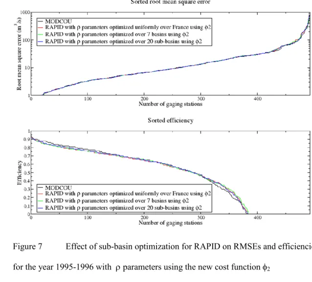
In order to estimate the effect of more spatial variability in the optimization of RAPID 347
parameters, the parameter estimation was done on different basins and sub-basins. Figure 348
7 shows the sorted Nash efficiencies and RMSEs obtained with three degrees of spatial 349
variability of optimization using 2as the cost function. These spatial variabilities 350
include “France” which has uniform parameters over the whole domain, “basins” for the 351
7 river basins of Figure 5a) (Adour, Garonne, Loire, Seine, Meuse, Rhône and Hérault) 352
and “sub-basins” where the major river basins have been divided into 20 sub-basins as 353
shown in Figure 5b). The increase in spatial variability of optimization increases the 354
efficiency while the RMSE remains almost constant, but the increase in efficiency is 355
limited compared to that triggered by a change in the cost function. The values of 356
parameters kand x obtained with the parameter estimation procedure using the second
357
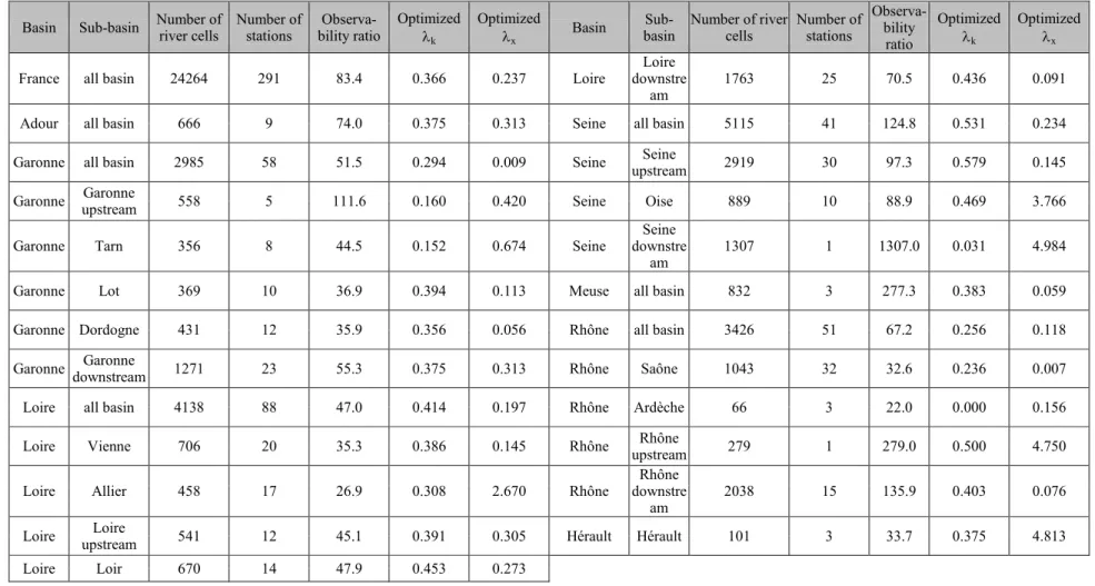
cost function are shown in Table 2. 358
The number of gaging stations in a basin can be divided by the number or river cells in 359
the basin to calculate an observability ratio O, as done in Table 2. This ratio ranges from
360
22
O on the Ardèche River to O1307downstream of the Seine River, showing a wide
361
spread in density of observations. The Seine River, of great interest to the French 362
community, has a higher resolution and therefore more river cells in SIM-France than any 363
other basin – all the river cells are of size 1 km – which explains the lower observability 364
ratio. Unrealistically low results are obtained for k in the downstream part of the Seine
365
River and for the Ardèche River Basin. The former is explained by the limited amount of 366
stations used for optimization in the downstream part of the Seine River Basin (only one 367
station). The latter is due to the basin being small with regards to the number of gages 368
(leading to a low observability ratio) and therefore over-constraining the optimization 369
procedure. The observability ratio is therefore a key metric for the quality of the 370
optimization. These unrealistic values for k may partly explain why the effect of
371
optimization from 7 basins to 20 sub-basins is very limited. As expected, the 372
optimization procedure converges to the largest values of the parameter k for the Seine 373
and Loire rivers which are the slowest rivers. For each of the 7 major basins, the value of 374
k
is bounded by the value of kfor each of their corresponding sub-basins. Also, one 375
can notice that upstream parts of a basin are usually faster (lower k) than downstream 376
parts as can be seen for the upstream part of the Loire Basin, and for the Allier Basin 377
which are located in high topography areas. This shows that – as expected – topography 378
plays an important role in the travel time of flow waves. This motivates a final 379
experiment where RAPID model parameters are estimated based on topography as shown 380 in Equation (9). 381 382 , , [1, 24264] j k i j , j x 0.1 i j d j k x s (9) 383 384
This formulation of kj is adapted from Equation (1) which is used to determine the
385
location of isochrone zones. In the following, the parameterskj and xj of Equation (9)
386
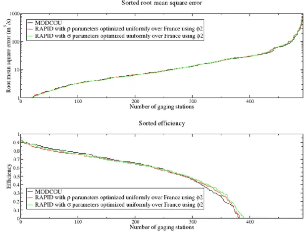
are referred to as parameters. Table 1 shows the average efficiencies and RMSEs 387
obtained with parameters using 1and 2uniformly over France, and with
parameters over the 7 major basins using 2. Figure 8 shows the sorted efficiencies
389
and RMSEs obtained with parameters using 1and 2uniformly over France. From
390
Table 1 and Figure 8 one can conclude that regardless of the optimization cost function 391
used, parameters allow to obtain better results than parameters. Therefore, taking 392
topography into account in the travel time of the flow wave is advantageous. Similarly, 393
regardless of the parameters used and of the spatial resolution of the optimization, 394
optimizing using 2allows obtaining better average results than with1. The average
395
results obtained using parameters and 2are comparable (slightly better) than those
396
obtained by the original routing module of SIM-France. One should note however, that 397
the best stations with MODCOU are better than the best with RAPID, while the worse 398
stations in MODCOU are worse than the worst in RAPID. This suggests a flattening of 399
the curves most likely due to equal treatment of all stations in the 2cost function. 400
Finally, regardless of the cost function used in optimization or the set of parameters 401
( and ) basin and sub-basin optimizations have a limited effect on overall 402
performance of RAPID. This suggests that increased inter-basin and intra-basin 403
variability of river routing parameters has little effect on efficiency or RMSE at the 404
spatial scale of France as it is modeled in SIM-France. 405
3.2. Comparison of routing schemes over 10 years
406
Over 1995-2005, only 3 gaging stations have a full daily record. Therefore, results 407
presented in this section are using stations with gaps in observations; efficiency and 408
RMSE are calculated only at times when measurements are available. A threshold of 409
70% of daily measurements available over 1995-2005 leads to selecting 493 gaging 410
stations. These stations differ slightly from the ones used in 1995-1996. Out of the 493 411
stations that have full daily record in 1996, 436 stations are included in the 1995-412
2005 period. Similarly, out of the best 291 stations that have full daily record in 1995-413
1996, 261 are included in 1995-2005. During 1995-2005, 427 out of the 493 stations 414
have a positive efficiency using the standard version of SIM-France. Table 1 shows 415
average statistics for 1995-2005 for the best 427 values for both efficiency and RMSE, 416
but similar patterns are found for all 493 values. The conclusions drawn in Section 3.2. 417
regarding the sets of parameters, the cost functions and the spatial resolution of the 418
optimization are still valid for the ten-year simulation. However, one should note that 419
over ten years, MODCOU performs slightly better than RAPID using the best set of 420
options. This may be explained by the slightly different stations used for the 5-month 421
optimization and for the ten-year study. However, five months of the first year seem to 422
be sufficient to capture RAPID parameters and allow comparable performance between 423
MODCOU and RAPID over ten years. Figure 9 shows the sorted efficiencies and 424
RMSEs obtained with MODCOU and with RAPID with parameters optimized 425
uniformly over France using 2. Globally the two models perform comparably although,
426
similarly to 1995-1996 results, the best stations are degraded and some stations with low 427
but positive efficiency are improved. Figure 10 shows observations and modeled 428
hydrographs during 1995-1996 and 1995-2005 for the Meuse River at Stenay (the 429
location of this station is shown in Figure 11) in which MODCOU and RAPID are almost 430
indiscernible. One should note, however, that in all the hydrographs plotted (not shown) 431
the timing of events differs slightly between the two models, none of which being 432
consistently better than the other regardless of the optimization options as expected from 433
results shown in Table 1 and Figure 9. 434
Figure 11 shows a spatial comparison of efficiencies obtained over France. 435
Improvements and degradations of statistical results between MODCOU and RAPID 436
have no particular spatial patterns. Overall, the discharge simulated by MODCOU and 437
RAPID are similar in RMSE and Nash efficiency. This similarity can be explained by 438
the strong dependence of discharge calculations on the lateral inflow forcing which is the 439
same for both river routing schemes. Furthermore, the routing equations used in 440
MODCOU and RAPID are comparable (the linear reservoir equation in SIM-France is a 441
simplified Muskingum equation, given x=0). The addition of RAPID to SIM-France can 442
be regarded as advantageous since RAPID provides with flow and volume of water in all 443
the cells of the river network separately and provides flexibility in the number and 444
location of river gages, which was not the case in the original version of SIM-France. 445
Also, the 30-min time step in RAPID allows potential comparisons with observations at 446
higher temporal resolution than the 3-hour time step of MODCOU. Finally, RAPID is 447
better suited than MODCOU for computation of river flow height in all grid cells of the 448
river network separately hence allowing the study of river-aquifer exchanges as shown in 449
Saleh et al. [2010; 2011]. 450
3.3. Influence of dams on river flow
451
RAPID does not have a specific physical model for treatment of dams. However, the 452
model is designed such that observations at gaging stations can easily be substituted for 453
upstream flow. This capability is not available in the routing scheme of MODCOU and 454
is useful for a gaging station located at the outlet of a dam because the flows discharging 455
from man-made infrastructures reflect human decisions. In France, the quality of flow 456
calculations at the outlet of the Rhône River (at Beaucaire) is influenced by the dam at 457
the outlet of Lake Geneva. Figure 12 demonstrates the influence of forcing with 458
observations at Pougny (downstream of the dam) on the calculation of flow at the outlet 459
of the Rhône River Basin. The gaging station a Pougny is the outlet of the “Rhône 460
upstream” basin in Figure 5b) and is also shown on Figure 11. The first year (August 1st 461
1995 – July 31st 1996) was used for this experiment. Forcing with observations at Lake 462
Geneva increases the Nash Efficiency from 0.49 to 0.62 at Beaucaire, the outlet of the 463
Rhône basin. 464
4. Conclusions
466
The river routing in SIM-France is done by MODCOU which uses groups of cells called 467
isochrone zones for its computations and does not directly compute flow and volume of 468
water for each cell of its quad-tree river network. The use of isochrones limits the 469
flexibility in the number and location of river gages. The work in this paper presents the 470
replacement of the river routing module in MODCOU by the river network model called 471
RAPID. Information on the network connectivity between the quad-tree river cells of 472
SIM-France is readily available in tables that relate upstream and downstream cells. 473
These tables can be used directly to create the network matrix of RAPID. A ten-year 474
study of river flow in Metropolitan France is presented comparing RAPID and the 475
routing module of MODCOU. An automated procedure for determining optimal model 476
parameters is available in RAPID and various options for the estimation of the 477
parameters are investigated. Sub-basin optimization increases model performance but its 478
influence is much smaller than the choice of the cost function. A cost function was 479
developed that normalizes the square-error between observations at each river gage and 480
RAPID computations by the average flow at the gage. This cost function is found to 481
globally increase the Nash efficiency of computed flow in all gages. We suggest that this 482
is due to the average flow having an influence on the computation of the Nash efficiency. 483
Therefore, the use of an appropriate criterion for quantifying the quality of river flow as 484
the cost function for the optimization procedure helps the betterment of model 485
computations. Also, flow wave celerities included in the temporal parameter of the 486
Muskingum method benefit from taking into account topography when compared to a 487
simple constant celerity formulation. Overall, the computation obtained with the addition 488
of RAPID are comparable to those of the original river routing module in SIM-France. 489
We consider the addition of RAPID as advantageous since flow and volume of water is 490
directly computed for each cell of the quad-tree river network. The formulation of 491
RAPID allows for easily substituting observed flows for the upstream calculated flow, 492
which is advantageous when considering a man-made infrastructure as was shown for the 493
Rhône River. 494
Acknowledgments
496
This work was partially supported by the French MinesParistech, by the French Agence 497
Nationale de la Recherche under the Vulnérabilité de la nappe du Rhin (VulNaR) project,
498
by the French Programme Interdisciplinaire de Recherche sur l'Environnement de la 499
Seine (PIREN-Seine) project, by the U.S. National Aeronautics and Space Administration
500
under the Interdisciplinary Science Project NNX07AL79G, by the U.S. National Science 501
Foundation under project EAR-0413265: CUAHSI Hydrologic Information Systems, and 502
by the American Geophysical Union under a Horton (Hydrology) Research Grant. 503
Thank you to Pere Quintana-Seguί for discussion about and for sharing data 504
corresponding to his work on SIM-France. Thank you to Firas Saleh and to Céline 505
Monteil for discussions on travel time within SIM-France. The authors are thankful to 506
the two anonymous reviewers and to the editor for their valuable comments and 507
suggestions that helped improved the original version of this manuscript. 508
References
510
Abdulla, F. A., D. P. Lettenmaier, E. F. Wood, and J. A. Smith (1996), Application of a 511
macroscale hydrologic model to estimate the water balance of the Arkansas Red River 512
basin, Journal of Geophysical Research-Atmospheres, 101, 7449-7459. 513
Boone, A., J.-C. Calvet, J. Noilhan, and euml (1999), Inclusion of a Third Soil Layer in a 514
Land Surface Scheme Using the Force-Restore Method, Journal of Applied Meteorology, 515
38, 1611-1630.
516
Cunge, J. A. (1969), On the subject of a flood propagation computation method 517
(Muskingum method), Journal of Hydraulic Research, 7, 205-230. 518
David, C. H., D. R. Maidment, G.-Y. Niu, Z.-L. Yang, F. Habets, and V. Eijkhout (2011), 519
River network routing on the NHDPlus dataset, Journal of Hydrometeorology, tentatively 520
accepted on 18 January 2011.
521
Decharme, B., H. Douville, A. Boone, F. Habets, and J. Noilhan (2006), Impact of an 522
Exponential Profile of Saturated Hydraulic Conductivity within the ISBA LSM: 523
Simulations over the Rhône Basin, Journal of Hydrometeorology, 7, 61-80. 524
Ducharne, A., C. Golaz, E. Leblois, K. Laval, J. Polcher, E. Ledoux, and G. de Marsily 525
(2003), Development of a high resolution runoff routing model, calibration and 526
application to assess runoff from the LMD GCM, Journal of Hydrology, 280, 207-228. 527
Durand, Y., E. Brun, L. Mérindol, G. Guyomarc'h, B. Lesaffre, and E. Martin (1993), A 528
meteorogical estimation of relevant parameters for snow models, Annals of Glaciology, 529
18, 65-71.
530
Habets, F., A. Boone, J. L. Champeaux, P. Etchevers, L. Franchisteguy, E. Leblois, E. 531
Ledoux, P. Le Moigne, E. Martin, S. Morel, J. Noilhan, P. Q. Segui, F. Rousset-532
Regimbeau, and P. Viennot (2008), The SAFRAN-ISBA-MODCOU 533
hydrometeorological model applied over France, Journal of Geophysical Research-534
Atmospheres, 113.
535
Leblanc, D., and J. P. Villeneuve (1978), Algorithme de schématisation des écoulements 536
d'un bassin versant 1-55 pp, Institut national de la recherche scientifique, Québec. 537
Leblois, E., and E. Sauquet (2000), Grid elevation models in hydrology. Part 2: 538
HydroDem technical note, 80 pp, Cemagref, Lyon. 539
Ledoux, E., G. Girard, G. de Marsily, J. P. Villeneuve, and J. Deschenes (1989), Spatially 540
Distributed Modeling: Conceptual Approach, Coupling Surface Water and Groundwater, 541
in Unsaturated Flow in Hydrologic Modeling Theory and Practice, edited by H. J. 542
Morel-Seytoux, pp. 435-454, Kluwer Academic Publishers. 543
Lohmann, D., R. NolteHolube, and E. Raschke (1996), A large-scale horizontal routing 544
model to be coupled to land surface parametrization schemes, Tellus Series a-Dynamic 545
Meteorology and Oceanography, 48, 708-721.
546
Lohmann, D., D. P. Lettenmaier, X. Liang, E. F. Wood, A. Boone, S. Chang, F. Chen, Y. 547
J. Dai, C. Desborough, R. E. Dickinson, Q. Y. Duan, M. Ek, Y. M. Gusev, F. Habets, P. 548
Irannejad, R. Koster, K. E. Mitchell, O. N. Nasonova, J. Noilhan, J. Schaake, A. 549
Schlosser, Y. P. Shao, A. B. Shmakin, D. Verseghy, K. Warrach, P. Wetzel, Y. K. Xue, 550
Z. L. Yang, and Q. C. Zeng (1998a), The Project for Intercomparison of Land-surface 551
Parameterization Schemes (PILPS) phase 2(c) Red-Arkansas River basin experiment: 3. 552
Spatial and temporal analysis of water fluxes, Global and Planetary Change, 19, 161-553
179. 554
Lohmann, D., E. Raschke, B. Nijssen, and D. P. Lettenmaier (1998b), Regional scale 555
hydrology: I. Formulation of the VIC-2L model coupled to a routing model, Hydrological 556
Sciences Journal-Journal Des Sciences Hydrologiques, 43, 131-141.
557
Lohmann, D., E. Raschke, B. Nijssen, and D. P. Lettenmaier (1998c), Regional scale 558
hydrology: II. Application of the VIC-2L model to the Weser River, Germany, 559
Hydrological Sciences Journal-Journal Des Sciences Hydrologiques, 43, 143-158.
560
Lohmann, D., K. E. Mitchell, P. R. Houser, E. F. Wood, J. C. Schaake, A. Robock, B. A. 561
Cosgrove, J. Sheffield, Q. Y. Duan, L. F. Luo, R. W. Higgins, R. T. Pinker, and J. D. 562
Tarpley (2004), Streamflow and water balance intercomparisons of four land surface 563
models in the North American Land Data Assimilation System project, Journal of 564
Geophysical Research-Atmospheres, 109, 1-22.
565
Maurer, E. P., G. M. O'Donnell, D. P. Lettenmaier, and J. O. Roads (2001), Evaluation of 566
the land surface water budget in NCEP/NCAR and NCEP/DOE reanalyses using an off-567
line hydrologic model, Journal of Geophysical Research-Atmospheres, 106, 17841-568
17862. 569
Nash, J. E., and J. V. Sutcliffe (1970), River flow forecasting through conceptual models 570
part I -- A discussion of principles, Journal of Hydrology, 10, 282-290. 571
Nelder, J. A., and R. Mead (1965), A Simplex Method for Function Minimization, The 572
Computer Journal, 7, 308-313.
573
Ngo-Duc, T., T. Oki, and S. Kanae (2007), A variable streamflow velocity method for 574
global river routing model: model description and preliminary results, Hydrol. Earth Syst. 575
Sci. Discuss., 4, 4389-4414.
Nijssen, B., D. P. Lettenmaier, X. Liang, S. W. Wetzel, and E. F. Wood (1997), 577
Streamflow simulation for continental-scale river basins, Water Resources Research, 33, 578
711-724. 579
Noilhan, J., and S. Planton (1989), A Simple Parameterization of Land Surface Processes 580
for Meteorological Models, Monthly Weather Review, 117, 536-549. 581
Oki, T., and Y. C. Sud (1998), Design of Total Runoff Integrating Pathways (TRIP) - A 582
Global River Channel Network, Earth Interactions, 2, 1-35. 583
Olivera, F., J. Famiglietti, and K. Asante (2000), Global-scale flow routing using a 584
source-to-sink algorithm, Water Resources Research, 36, 2197-2207. 585
Quintana-Seguỉ, P., P. Le Moigne, Y. Durand, E. Martin, F. Habets, M. Baillon, C. 586
Canellas, L. Franchisteguy, and S. Morel (2008), Analysis of near-surface atmospheric 587
variables: Validation of the SAFRAN analysis over France, Journal of Applied 588
Meteorology and Climatology, 47, 92-107.
589
Quintana-Seguỉ, P., E. Martin, F. Habets, and J. Noilhan (2009), Improvement, 590
calibration and validation of a distributed hydrological model over France, Hydrol. Earth 591
Syst. Sci., 13, 163-181.
592
Saleh, F. S. M., N. Flipo, F. Habets, A. Ducharne, L. Oudin, M. Poulin, P. Viennot, and 593
E. Ledoux (2010), CONTRIBUTION OF 1D RIVER FLOW MODELING TO THE 594
QUANTIFICATION OF STREAM-AQUIFER INTERACTIONS IN A REGIONAL 595
HYDROLOGICAL MODEL, paper presented at XVIII International Conference on 596
Computational Methods in Water Resources (CMWR 2010) 597
CMWR 2010, Barcelona. 598
Saleh, F. S. M., N. Flipo, F. Habets, A. Ducharne, L. Oudin, P. Viennot, and E. Ledoux 599
(2011), Modeling the impact of in-stream water level fluctuations on stream-aquifer 600
interactions at the regional scale, Journal of Hydrology, accepted. 601
SCHAPI (2008), Banque HYDRO, Service Central d'Hydrométéorologie et d'Appui à la 602
Prévision des Inondations available online at http://www.hydro.eaufrance.fr/index.php. 603
USEPA, and USGS (2007), NHDPlus User Guide, available online at 604
http://www.horizon-systems.com/nhdplus/documentation.php. 605
Wetzel, S. (1994), A hydrological model for predicting the effects of climate change, 85 606
pp, Princeton University, Princeton. 607
608 609
Table 1 Average efficiencies and average root mean square errors computed for MODCOU and for RAPID with 7 different 610
sets of parameters. The best 382 values are used for 1995-1996 and the best 427 values are used for 1995-2005. 611
1995-1996 1995-2005
Best 382 values Best 427 values Vector of
parameters used in optimization
Optimization
cost function Spatial optimization Model
Average
efficiency Average RMSE (m3/s) Average efficiency
Average RMSE (m3/s)
N/A N/A N/A MODCOU 0.617 8.37 0.650 12.67
1 France RAPID 0.581 8.85 0.614 13.64 2 France RAPID 0.611 8.39 0.638 13.07 2 7 basins RAPID 0.615 8.40 0.640 13.06 2 20 sub-basins RAPID 0.615 8.38 0.637 13.04 1 France RAPID 0.602 8.63 0.632 13.25 2 France RAPID 0.620 8.37 0.647 12.91 2 7 basins RAPID 0.624 8.32 0.646 12.92 612
Table 2 Results of optimization procedure using parameters and the 2 cost function 613
Basin Sub-basin Number of river cells Number of stations bility ratio Observa- Optimized
k
Optimized
x Basin
Sub-basin Number of river cells Number of stations
Observa-bility ratio Optimized k Optimized x
France all basin 24264 291 83.4 0.366 0.237 Loire downstreLoire
am 1763 25 70.5 0.436 0.091
Adour all basin 666 9 74.0 0.375 0.313 Seine all basin 5115 41 124.8 0.531 0.234
Garonne all basin 2985 58 51.5 0.294 0.009 Seine upstream Seine 2919 30 97.3 0.579 0.145
Garonne upstream Garonne 558 5 111.6 0.160 0.420 Seine Oise 889 10 88.9 0.469 3.766
Garonne Tarn 356 8 44.5 0.152 0.674 Seine downstreSeine
am 1307 1 1307.0 0.031 4.984
Garonne Lot 369 10 36.9 0.394 0.113 Meuse all basin 832 3 277.3 0.383 0.059
Garonne Dordogne 431 12 35.9 0.356 0.056 Rhône all basin 3426 51 67.2 0.256 0.118
Garonne downstream Garonne 1271 23 55.3 0.375 0.313 Rhône Saône 1043 32 32.6 0.236 0.007
Loire all basin 4138 88 47.0 0.414 0.197 Rhône Ardèche 66 3 22.0 0.000 0.156
Loire Vienne 706 20 35.3 0.386 0.145 Rhône upstream Rhône 279 1 279.0 0.500 4.750
Loire Allier 458 17 26.9 0.308 2.670 Rhône downstreRhône
am 2038 15 135.9 0.403 0.076
Loire upstream Loire 541 12 45.1 0.391 0.305 Hérault Hérault 101 3 33.7 0.375 4.813
Loire Loir 670 14 47.9 0.453 0.273
Captions to illustrations
615 616 617
618
619
Figure 1 Structure of SIM-France, from Habets et al. [2008] 620
622
Figure 2 France and computational domain of SIM-France 623
625
Figure 3 Surface and river isochrone zones in Ardèche Basin in MODCOU within 626
SIM-France 627
629
Figure 4 Map of the parameter used for river routing in MODCOU within SIM-630
France 631
633
Figure 5 Basins treated independently during optimization of RAPID parameters in 634
SIM-France. a) Seven major river basins. b) Twenty sub-basins 635
637
Figure 6 Comparison of sorted RMSEs and efficiencies for the year 1995-1996 638
between MODCOU and RAPID with parameters optimized uniformly over France 639
using the original cost function and using the new cost function
640
641 642
643
Figure 7 Effect of sub-basin optimization for RAPID on RMSEs and efficiencies 644
for the year 1995-1996 with parameters using the new cost function
645 646
647
Figure 8 Effect of set of parameters and for RAPID on RMSEs and efficiencies 648
for the year 1995-1996 using the new cost function 2 uniformly over France 649
650
Figure 9 Comparison of sorted RMSEs and efficiencies for the years 1995-2005 651
between MODCOU and RAPID with parameters optimized uniformly over France 652
using the new cost function 2 653
654
Figure 10 Comparison of 1995-1996 and 1995-2005 hydrographs for the Meuse 655
River at Stenay obtained by MODCOU and RAPID with parameters optimized 656
uniformly over France using the new cost function 2 657
658
Figure 11 Spatial difference of efficiencies obtained for the years 1995-2005 659
between RAPID using parameters optimized uniformly over France using the new cost 660
function 2 and MODCOU
661 662
663
Figure 12 Comparison of RAPID discharge calculation at the outlet of the Rhône 664
River (at Beaucaire) with and without forcing at the outlet of Lake Geneva (at Pougny). 665

![Figure 1 Structure of SIM-France, from Habets et al. [2008]](https://thumb-eu.123doks.com/thumbv2/123doknet/8287492.279172/36.918.246.663.152.633/figure-structure-sim-france-habets-et-al.webp)