Bramoullé : Department of Economics, CIRPÉE and GREEN, Université Laval
Rogers: MEDS, Kellogg School of Management, Northwestern University
We thank Andrea Galeotti, Sanjeev Goyal, Matthew Jackson, Bruno Strulovici, and Adrien Vigier, as well as seminar participants at the First Transatlantic Theory Workshop (Paris), The University of Essex, and Cambridge University for helpful comments and conversations. This research uses data from Add Heath, a program project designed by J. Richard Udry, Peter S. Bearman, and Kathleen Mullan Harris, and funded by a grant P01-HD31921 from the National Institute of Child Health and Human Development. Persons interested in obtaining data files from Add Heath should contact Add Health, Carolina Population Center, 123 W. Franklin Street, Chapel Hill, NC 27516-2524 ([email protected]).
Cahier de recherche/Working Paper 09-03
Diversity and Popularity in Social Networks
Yann Bramoullé Brian W. Rogers
Abstract:
Homophily, the tendency of linked agents to have similar characteristics, is an important feature of social networks. We present a new model of network formation that allows the linking process to depend on individuals types and study the impact of such a bias on the network structure. Our main results fall into three categories: (i) we compare the distributions of intra- and inter-group links in terms of stochastic dominance, (ii) we show how, at the group level, homophily depends on the groups size and the details of the formation process, and (iii) we understand precisely the determinants of local homophily at the individual level. Especially, we find that popular individuals have more diverse networks. Our results are supported empirically in the AddHealth data looking at networks of social connections between boys and girls.
Keywords: Social networks, Network formation, Homophily, Diversity
I
Introduction
A thorough understanding of homophily is essential to the study of social and economic net-works. Homophily is the tendency for similar individuals to be connected to each other. While its prevalence has been documented empirically across many contexts, it has been relatively neglected, so far, in theoretical studies on networks. Homophily implies positive correlations in the characteristics of individuals linked to each other in a network, and such correlations may have substantial implications for the operation of various processes within the network. The outcomes regarding diffusion of information, technologies, and disease, behavioral outcomes in games of strategic complements or substitutes played in a networked society, and observational learning may all depend non-trivially on homophilic aspects of the network.
We develop a model of network formation in order to advance our understanding of ho-mophily. The framework allows us to keep track of the characteristics of individuals, measured as a group identity, and how they relate to their pattern of connections in the network. We are able to uncover some systematic relationships that are not obvious a priori. We are especially in-terested in the relationship between degree (number of connections), degree distributions across society, and the extent of local and aggregate homophily. To investigate these relationships, we extend the model of Jackson & Rogers (2007). This model provides an ideal starting point as it is both tractable and able to replicate most empirically documented features of social networks
except for homophily. This paper overcomes this limitation, yielding new insights and empirical
predictions.
Notably, we show that individuals with a higher degree should have more balanced
neighbor-hoods. This prediction turns out to be strongly supported empirically, when looking at gender
bias in friendship networks among adolescents. Using Add Health data, we find that in high school, boys and girls who receive more friendship nominations indeed have a much more diverse network of friends.
This paper contributes to a growing literature studying stochastic models of network forma-tion. Until very recently, most studies have focused mainly on degree distributions and other summary statistics of the network independent of individuals’ types or other characteristics, see
for instance Barabasi and Albert (1999), Chung & Lu (2002a,b), Jackson & Rogers (2007), New-man (2003, 2004), and Watts and Strogatz (1998). Building on this literature, we acknowledge the empirical importance of community structure and investigate its interplay with the other network features.
Two other recent papers have started to tackle these issues.1 Currarini, Jackson, and Pin (2008) study a matching process of friendship formation. They document several empirical patterns of homophily and explain them through a combination of biases with respect to choice (preferences) and chance (opportunities presented by the matching process). By design, their model does not allow degree to vary across individuals. This makes their entire analysis quite different from ours. Interestingly, however, a number of their predictions are also supported by our model. Jackson (2008) incorporates homophily into the random graph model of Chung & Lu (2002a,b).2 Again by design, homophily cannot vary with degree in this approach. Also, degree distributions constitute an outcome of our model while they are an input of Jackson (2008). Thus, our analysis and these two papers study homophily patterns in networks from three distinct and rather complementary points of view. In particular, we provide the first study of the relationship between homophily and individual’s degree.
We now describe our model in more detail. As in Jackson & Rogers (2007), individuals are born sequentially. Upon entry, an individual meets others in two distinct ways: at random and through network-based search. The network-based search allows individuals to meet the neighbors of their randomly met partners. In either case, conditional on a meeting taking place, a connection is formed with some probability. We depart from Jackson & Rogers (2007) by assigning individuals a group identity or label, and allowing the meeting process to be affected by group identity.3 Specifically, we assume that random meetings take place in either of two “locations” and that nodes of a specific group are exogenously more likely to be in a specific location. These locations could indeed be spatially based, such as geographic neighborhoods, or
1The study of homophily dates back to Lazarsfeld and Merton (1954); McPherson, Smith-Lovin and Cook
(2001) document observations of homophilic biases in dozens of studies.
2Jackson & Golub (2008) use this extension to study how homophily affects communication dynamics in
networks, demonstrating one way in which homophilic structure impacts outcomes.
3A different approach by Vigier (2008) extends the Jackson & Rogers (2007) model to allow link formation to
instead they could represent more general social interaction settings, including church and club memberships. We leave the rest of the network formation process unchanged and study how this bias in random meetings propagates through the system.4 This allows us to develop a clean understanding of homophily patterns induced by random meeting biases.5
We obtain three sets of theoretical results about homophily, degree distributions and the relation between homophily and degree, which we now outline.
First, we study how the exogenously taken bias in random meetings relates to the observed homophily in society as the population grows large. Our main finding here is that network search has a dampening effect on homophily. Meeting “friends of friends” opens up more possibilities for diverse relationships. Thus, network homophily decreases as the ratio of search-based to random meetings increases. We also look at the relationship between the relative homophily within a particular group and the relative size of that group in society. As in Currarini, Jackson, and Pin (2008), we find that this relation exhibits an inverted U-shape. It is remarkable that two models built on very different premises lead to this similar conclusion.
Second, we use the mean-field approximation to characterize the degree distributions of the social network. In the presence of community structure, we are interested in seven distributions rather than only one. For instance, we can keep track of the distribution of the number of links that boys have with girls, boys have with boys, and so forth. We study the shapes and comparative statics of these distributions. We show that they all have a scale-free upper tail with
a common exponent, even though the distributions themselves are not scale-free. We also derive
a number of comparisons across distributions using first-order stochastic dominance. Finally, the distribution of total in-degree for two populations are identical, independent of the relative group sizes and extent of location biases.
Third, we examine the relationship between an individual’s degree and the homophily in its immediate neighborhood. That is, we examine how the number of links of a node is related to the proportion of its neighbors that belong to the same group. Our main result here is that
4We do not introduce a group-dependent bias in link formation conditional on meeting. We return to discussing
this issue in the conclusion.
5In fact, we derive many of our results under a general representation of random meeting biases that
this local homophily decrease with an individual’s degree. In other words, nodes with a higher degree have more diverse networks. In the limit, the homophilic bias completely disappears as degree becomes very high, independent of the bias in random meetings. In addition, we find that this decrease takes place at a decreasing rate and is less pronounced in larger groups. This analysis provides the first comprehensive results relating homophily and degree distributions in social networks.
Our final contribution is to bring data to bear on these novel predictions. We look at gender and friendship networks among high school students in the U.S. provided in the AddHealth data. First, we find that the distribution of in-degree is remarkably similar for boys and girls. Second, we test the hypotheses that individual homophily is decreasing and convex in degree, and that the relationship is more dramatic in smaller groups. Regressions yield highly significant coefficients for our variables of interest, all with the predicted signs. These findings may have important consequences for the debate on gender composition and social interactions at school. The paper proceeds as follows. The next section describes the formal model. Section III contains the fundamental results on homophily. Section IV derives degree distributions for the network under the mean-field approximation, and presents a number of relationships across de-gree distributions. Section V describes how local homophily varies with dede-gree, which highlights the importance of studying a model with non-trivial degree distributions. Section VI presents the results of the empirical analysis of homophily in networks, and relates the findings to the predictions of our model. The final section offers concluding remarks. An appendix contains some supplemental formal results.
II
A model of community structure in social networks
We introduce the notion of community structure to a version of the model from Jackson & Rogers (2007), which we now describe.
Nodes enter the world one at a time and are indexed by their date of birth t = 1, 2, .... Entering nodes meet some of the existing nodes via two processes: at random and through
network-based search. Some of these meetings result in a relationship, modeled as a directed link from the new node to the older node. In this case we refer to the older node as an “out-neighbor” of the entering node, and conversely to the entering node as an “in-“out-neighbor” of the older node.
Specifically, each entering node first meets mr existing nodes through the random meeting
process, where the meetings are drawn uniformly and independently at random from the set of existing nodes. We sometimes refer to nodes so met as parents. It then meets an additional
ms nodes chosen uniformly and independently at random from the set of nodes consisting of
the union of parents’ out-neighbors. Finally, it independently forms a directed out-link with probability p with each of these mr+ ms nodes that it has met. The expected number of links
thus formed is m = p(ms+ mr); r = mr/ms represents the ratio of the number of connections
formed through the random process versus through the search process.
Our key assumption is that individuals are endowed with types, which we refer to as group membership, and that group identity (potentially) impacts the meeting process. Specifically, nodes belong to one of two groups g1 and g2. At birth they are independently assigned to g1 with probability q and to g2 with probability 1 − q. Thus at time t, the expected number of nodes in g1 is qt and in g2 is (1 − q)t.
We suppose that there are two locations L1 and L2. Each node that enters goes to one location, and meets mr nodes uniformly at random among all individuals present at this location.
All biases in the meeting process are captured by the parameter γ ∈ [.5, 1], which represents the probability that a gi node goes to location Li, i = 1, 2.6 Thus, it is simply the resulting composition of types in the two locations that permits any group-dependent biases in the model. Once at a particular location, all random meetings ignore types. In addition, both the search-based meetings and the probabilities of forming a link conditional on a meeting taking place ignore types and are exactly as described above.
At any time t, the expected number of g1 nodes at L1 is qγt, while the expected number of 6Actually, the analysis below assumes away some implicit correlations in the meetings process described here.
To account for this, one can instead assume that each new node in gi spends a proportion γ of his time in Li,
g2 nodes in L1 is (1 − q)(1 − γ)t. Thus, the proportion of g1 nodes in L1 is qγ
qγ+(1−q)(1−γ) while the
proportion of g1 nodes in L2 is q(1−γ)
q(1−γ)+(1−q)γ. Defining bi as the proportion of a gi node’s random
meetings that are within its own group, i = 1, 2, this yields:
b1 = γ
qγ
qγ + (1 − q)(1 − γ) + (1 − γ)
q(1 − γ)
q(1 − γ) + (1 − q)γ (II.1)
and b2 is obtained by symmetry exchanging q and 1 − q.
Once the population sizes, q, have been fixed, a single parameter, γ, determines how the random meeting biases, b1 and b2, vary. However, we are able to prove many of our results in a more general setting in which b1and b2, taken as primitives of the model rather than implications of location-based biases, can vary freely with respect to each other. In these cases, the process can be viewed as follows. Independently for each random meeting of an entering node of type
gi, a coin is first flipped to determine the group of the individual to be met, with probability b i
of choosing another individual from gi. Then, conditional on the group, an individual is selected
uniformly at random from the appropriate type.
Whether or not the meeting process is location-driven, we can think of any resulting biases as being described by b1 and b2. Moreover we must interpret b1and b2 relative to q, which measures the relative proportions of the two groups. In particular, we say that there is no homophilic bias if b1 = q and b2 = 1 − q. In that case, the proportions of random meetings within and between the groups simply reflects the relative sizes of the groups in the population. When biases are driven by locations, this corresponds to γ = 1
2. In contrast, we say that there is homophilic bias if b1 > q and b2 > 1 − q and random meetings are relatively biased towards own group. This occurs whenever γ > 1
2. At the extreme when γ = 1, so that b1 = b2 = 1, individuals meet others only from their own group.7
7Notice that in general we can consider heterophilic bias, where b
1 < q and b2 < 1 − q, although this is not
possible when biases are location driven. We rule out values of γ < 1/2 without loss of generality since they correspond to cases we already consider by relabeling the locations.
III
Homophily in relationships
First, we want to understand how homophilic bias in random meetings relates to the homophily observed in the resulting network. In particular, for a given specification, does increasing the proportion of search-based meetings amplify or mitigate the homophilic bias?
Formally, define group i network homophily, βi, as the expected proportion of the links formed
by a new node in gi that are with other nodes in gi. A priori β
i depends on t, but we can show
that βi quickly reaches a steady-state, in which case βi measures the proportion of the links
formed by all nodes in gi that point to nodes also in gi. Given values of b
1 and b2, β1 and β2 must solve the following system of equations at the steady-state:
β1m = p [b1mr+ (β1b1+ (1 − β2)(1 − b1))ms]
β2m = p [b2mr+ (β2b2+ (1 − β1)(1 − b2))ms] .
To see why, consider, for instance, the first equation. The left hand-side is the expected number of links that a new node in g1 forms with existing nodes in g1. On the right hand side, this number is expressed as the sum of the expected number of links in g1 formed at random (pb
1mr)
and through search. Among all the parents’ out-neighbors, what proportion of them are in
g1? A fraction b
1 of parents are in g1, and the proportion of their out-neighbors in g1 is (by definition) β1, while the remaining proportion 1 − b1 of parents in g2 have a proportion 1 − β2 of their out-neighbors in g1. Since the new node has m
s search-based meetings, we get the second
term in the equation. Rewriting these equations as functions of the ratio of random to search meetings, we get
β1(1 + r) = b1r + β1b1+ (1 − β2)(1 − b1)
β2(1 + r) = b2r + β2b2+ (1 − β1)(1 − b2)
β1 = b1r + 1 − b2 r + 1 − b1+ 1 − b2 ; β2 = b2r + 1 − b1 r + 1 − b2+ 1 − b1 . (III.2)
Proposition 1 Network homophily βi is always strictly increasing in bi and strictly decreasing in
b−i. Under a homophilic bias, it is strictly increasing in r and strictly less than the corresponding
homophilic bias bi.
Proof. The results follow from examining the partial derivatives of equations (III.2). First,
∂βi
∂bi > 0 if and only if r(r + 1 + 1 − b−i) + 1 − b−i > 0, which holds since r > 0 and b−i < 1. Next, ∂βi
∂b−i < 0 if and only if r + 1 − bi > bir, which holds as r + 1 − bi > r > b1r. Now assume there
is a homophilic bias, i.e., b1 > q and b2 > 1 − q. Thus b1+ b2 > 1. We have ∂βi∂r > 0 if and only if b1+ b2 > 1, and similarly βi < bi if and only if b1+ b2 > 1, completing the proof.
Notice that Proposition 1 does not rely on assuming that the homophilic biases are driven by location choices, and is true for any specification of b1 and b2.
The intuition is as follows. As bi increases, new gi nodes form a higher proportion of their
randomly met out-links with other gi nodes. These parent nodes also have a higher proportion
of gi out-neighbors, and so β
i increases. As b−i decreases, the random meeting process for gi
nodes is unaffected. Since some of the parent nodes will be from g−i, and these nodes now have
a higher proportion of gi neighbors, gi nodes will form a higher proportion of within-group links.
Now consider the case of homophilic bias. Since the resulting network homophily is increasing in r, the meetings formed through the search process have a dampening effect on homophily. This phenomenon is central to our analysis and deserves some elaboration. Recall that through search a node has access to all the parents’ neighbors. This includes, of course, the neighbors of parents in the other group which, because of homophily, tend to also belong to the other group. Thus, search gives access to many nodes of the other group. In short, meeting the friends of distinct friends opens up possibilities for diverse relationships. Search acts here as a countervailing force with regards to the original bias in random meetings.
Introduce β10= 1−b1−b1+1−b2 2 as the limiting (group 1) network homophily when r tends to zero, or mr ¿ ms. It is the lowest possible value of network homophily for given values of q, b1 and
b2.8 When biases are location-driven, β10 = q and hence a homophilic bias implies network homophily.9 However, when b
1 and b2 can vary freely, the dampening effect can be so strong as to overturn the homophilic bias, resulting for instance in β2 < 1 − q.10
Next, we want to study relative homophily H1 = (β1− q)/(1 − q) and H2 = (β2− (1 − q))/q. Relative homophily is positive when a group forms a higher proportion of its links within the group than would be implied by the population sizes, and is normalized to have a maximal value at unity. The first result shows how relative homophily changes as the composition of society varies.
Proposition 2 H1 is symmetric around q = 1/2. It is equal to zero at q = 0 and 1; it increases
from q = 0 to q = 1/2, and decreases from q = 1/2 to q = 1, and is concave.
Proof. Substituting from equation (II.1), we have
H1(q) =
(1 − 2γ)2rq(1 − q)
rq(1 − q) + (1 + (1 − 2q)2r)γ(1 − γ)
From this expression, it is easily verified that H1(q) = H1(1 − q) and that H1(0) = H1(1) = 0. The first derivative of H1 is
∂H1(q)
∂q =
(1 − 2q)r(r + 1)(2g − 1)2γ(1 − γ) ((r + 1)γ(1 − γ) + (2γ − 1)2qr(1 − q))2,
which has the same sign as 1 − 2q, proving that H1 is increasing below q = 1/2 and then decreasing. To show concavity, write the second derivative as
∂2H 1(q)
∂q2 =
2γ(1 − γ)(2γ − 1)2r(r + 1) ∗ (r(3q2− 3q + 1) − γ(1 − γ)(3r(2q − 1)2− 1))
−r3(γ(1 − γ)((2q − 1)2+ 1) + q(1 − q))3 . The denominator is negative, and the term in the numerator before the asterisk is positive, so
H1 is concave if and only if r(3q2− 3q + 1) − γ(1 − γ)(3r(2q − 1)2− 1) > 0. Dividing by r and 8We show below that this parameter also plays a crucial role in degree distributions.
9Conversely, we can show that the model always exhibit network inbreeding homophily only when β 10 = q
and β20= 1 − q.
10Interestingly, network heterophily can only emerge for one of the two groups. This echos Proposition 3 in
rearranging, we must show that γ(1 − γ)(3(2q − 1)2− 1/r) + 3q(1 − q) < 1. γ(1 − γ) ≤ 1/4 and
−1/r ≤ 0; using these inequalities and collecting terms proves the result.
Thus, in the extreme cases where one group dominates society, relative homophily disappears. In all other cases, however, relative homophily is positive, and is strongest for intermediate size groups, reaching a maximum when the groups have equal size. Interestingly, the equilibrium mixing model of Currarini, Jackson, and Pin (2008) generates an analogous result through a very different analysis, and their result is supported empirically looking at racial composition in the AddHealth data.
The next result shows how relative homophily responds to changes in the meeting process. Proposition 3 H1(q) is shifted up by an increase in r or by an increase in γ.
Proof. The relevant derivatives are
∂H1 ∂r = (1 − 2γ)2γ(1 − γ)q(1 − q) (rq(1 − q) + γ(1 − γ)(1 + (1 − 2q)2)r)2 ∂H1 ∂γ = (2γ − 1)q(1 − q)r(1 + r) (rq(1 − q) + γ(1 − γ)(1 + (1 − 2q)2)r)2, both of which are easily verified as being positive.
That is, for a given society and homophilic biases, decreasing the role of search-based meetings increases relative homophily. This results from the “dampening effect” of search-based meetings on network homophily. The more prevalent search-based meetings are in the formation process, the lower homophily will be, as “friends of friends” are less likely to be of the same type than are individuals met through the biased random meetings. Since there is a homophilic bias whenever
γ > 1/2, this result is consistent with Proposition 1 which describes network homophily more
generally. Finally, increasing the location bias, all else equal, increases relative homophily for any value of r, since this is the parameter thats controls the extent to which random meetings are exogenously biased.
IV
Relationships among the distributions of links
In this section, we make use of the powerful mean-field approximation to study degree distribu-tions. Even with only two groups, the distribution of links becomes substantially more complex than the Jackson & Rogers (2007) case as nodes can connect to both same and different type nodes, and one wants to keep track of the different kinds of links. We focus on the distributions of in-degrees, as out-degrees are essentially homogenous, with all nodes of the same type forming their out-links according to the same (stochastic) rule. In this context, we can keep track of
seven different degree distributions rather than one. Define Fij as the distribution of the
in-degrees of type gi nodes paying attention only to links coming from nodes of type gj, i, j = 1, 2.
Then F1 and F2 are the standard in-degree distributions of g1 and g2 nodes (ignoring the types of in-neighbors), and finally F is the total in-degree distribution of the entire society.
We emphasize that we are able to derive many of the results of this section for arbitrary specifications of biases b1 and b2. It is not until we get to Proposition 8 that we specialize to consider biases driven by γ and location choices.
Consider a node i ∈ g1. Let kt
11 denote the number of in-links of i with other nodes from group g1 at time t, while kt
12 is the number of in-links with nodes from the other group. Then,
kt
1 = k11t + kt12 is the total in-degree of node i at time t.
Now consider the individual entering at time t > i. What are the probabilities that this node forms a link with i, and hence that kt
11 or kt12 increase by one unit?
P (kt+111 = kt11+ 1) = qp(b1mr qt + ms mmr (k11t b1mr qt + k t 12 (1 − b1)mr (1 − q)t ))
The new node is in g1 with probability q, and forms a link with i conditional on having met him with probability p. It meets i at random with probability b1mr (number of random meetings)
divided by qt (number of nodes in g1); or it meets i through search. In this case, one of i’s in-neighbors must have been found randomly, which happens with probability kt
11b1qtmr+kt12(1−b(1−q)t1)mr. To see this, note that i has kt
11 out-neighbors in g1, each of which is met at random by t with probability b1mr
with probability (1−b1)mr
(1−q)t . Given that one of i’s out-neighbors was met at random by t, i is met through search with probability ms
mmr, since t meets ms nodes through search and has mr parent
nodes to search from, each of whom has on average m out-neighbors. By similar reasoning we get P (kt+1 12 = kt12+ 1) = (1 − q)p( (1 − b2)mr qt + ms mmr (kt 11 (1 − b2)mr qt + k t 12 b2mr (1 − q)t)). Thus, under a continuous mean-field approximation, kt
11 and kt12 satisfy the following system of differential equations with initial conditions ki
11= k12i = 0 ∂kt 11 ∂t = m r 1 + rb1 1 t + 1 1 + rb1 kt 11 t + 1 1 + r(1 − b1) q 1 − q kt 12 t ∂kt 12 ∂t = m r 1 + r(1 − b2) 1 − q q 1 t + 1 1 + rb2 kt 12 t + 1 1 + r(1 − b2) 1 − q q kt 11 t
Solving these equation provides the expressions for degree growth. We have Proposition 4 k11 = mr[β10( t i) 1/(1+r)+ (1 − β 10)( t i) (b1+b2−1)/(1+r)− 1] k12 = mr 1 − q q β10[( t i) 1/(1+r)− (t i) (b1+b2−1)/(1+r)]
Proof. See the Appendix.
To obtain the total in-degree of node i as a function of time, we simply sum the two equations of Proposition 4. This yields k1 = mr[βq10(ti)1/(1+r)+ (1 −βq10)(ti)(b1+b2−1)/(1+r)− 1]. We can now see how results of Jackson & Rogers (2007) are obtained as special cases. Two specific situations give us back the same expression as in the model without homophily. First if there is no homophilic bias. This corresponds to b1 = q and b2 = 1 − q, hence β10 = q and b1 + b2 = 1 which leads to k1 = mr[(ti)1/(1+r) − 1]. Second if, in contrast, the homophilic bias is extreme and nodes do not meet any nodes from the other group. Then, b1 = b2 = 1 which also leads to k1 = mr[(ti)1/(1+r)− 1]. Thus, Proposition 4 indeed implies Theorem 1 in Jackson & Rogers
(2008).11
To obtain F11, observe that F11(k) = 1 − i/t, which means that t/i = 1/(1 − F11(k)). This defines F11 implicitly as a function of k, and a similar method works for the other distribu-tions. While these equations do not usually yield closed-form solutions, they still allow us to derive important properties of the degree distributions. Our first such result orders the degree distributions as the number of out-links is varied.
Proposition 5 Fix q, b1, b2 and r. Let Fij be the distributions corresponding to the parameter
m and let F0
ij be the distributions corresponding to m0. If m0 > m, then Fij0 strictly first-order
stochastically dominates Fij, for every i, j = 1, 2.
Proof. It is enough to show that the expressions for the kij are increasing in m, which follows
directly from Proposition 4. We can then apply Lemma 1 (see the Appendix) to prove the result.
This implies the result in Theorem 7 of Jackson & Rogers (2007), where the case of only one group is considered. Next we turn to approximating the upper tail of the various degree distributions. It turns out that all of the degree distributions have similar upper tails, and in particular, that they tend to a scale-free distribution with exponent −(1 + r).
Proposition 6 When k is large,
ln(1 − F11(k)) ∼ ln(mrβ10) − (1 + r) ln(k) ln(1 − F12(k)) ∼ ln(mrβ10 1 − q q ) − (1 + r) ln(k) ln(1 − F1(k)) ∼ ln(mrβ10 1 q) − (1 + r) ln(k)
Proof. From Proposition 4, we can obtain the implicit equation defining F11(k) :
k = mr[β10(1 − F )−1/(1+r)+ (1 − β10)(1 − F )−(b1+b2−1)/(1+r)− 1], 11Both situations are of course not equivalent. For instance, we see that k
11= qk1when there is no homophilic
which we write as k = mrβ10(1 − F )−1/(1+r)[1 + ε(k)], where ε(k) = 1−β10 β10 (1−F ) (2−b1−b2)/(1+r)−(1−F )1/(1+r). Since b 1+b2 < 2, we have limk→∞ε(k) =
0. Taking the log we get:
ln(1 − F ) = (1 + r) ln(mrβ10) − (1 + r) ln k + η(k),
where η(k) = (1 + r) ln(1 + ε(k)), and so η(k) tends to zero as k tends to infinity. Similar reasoning works for the other distributions.
This result says that all seven distributions have a fat upper tail following a power law with exponent −(1+r). In other words, the relative proportions of links coming to nodes of either type from nodes of either type are all identical for sufficiently high degree. This provides a particularly sharp and empirical testable prediction of the model. The upper tails of the distributions for nodes in group g2 can be derived analogously.
Next, we ask how Fi1 and Fi2 compare to each other. That is, we focus on one group gi, and
compare the distributions for that group of in-degrees coming from each of the two groups. We find that the answer very much depends on the size of group i.
Proposition 7
(i) When q > 1/2, F11 FOSD F12.
(ii) If q > 1/2 and b1+ b2 < 2, then F22 never FOSD F21.
(iii) F21 FOSD F22 if and only if (2q − 1)(1 − b1) ≥ (1 − q)(b1+ b2− 1).
Proof. For (i), use Proposition 4 to write
k11 = mrβ10 · (t i) 1/(1+r)− (t i) (b1+b2−1)/(1+r) ¸ + mr · (t i) (b1+b2−1)/(1+r)− 1 ¸ k12 = mrβ10 µ 1 − q q ¶ · (t i) 1/(1+r)− (t i) (b1+b2−1)/(1+r) ¸ .
equation is non-negative. Thus k11(t/i) > k12(t/i) for all t ≥ i, which allows us to apply Lemma 1.
Now consider the expressions for k22and k21obtained from the above equations by switching the group labels 1 and 2 and switching q with 1 − q. When q > 1/2 (meaning g1 is the majority group) then 1−qq > 1, and when b1+ b2 < 2 (meaning there is at least some inter-group linking) then for large values of t/i the second term in the expression for k22 becomes negligible, in which case k22< k21 in the upper tail, proving (ii) by application of Lemma 1.
For (iii), introduce the function ψ(x) = qβ20[xα1 − xα2] − (1 − q)[β20xα1 + (1 − β20)xα2 − 1], where α1 = 1+r1 and α2 = b1+b1+r2−1. Note that ψ(x) ≥ 0 if and only if k21(x) ≥ k22(x). Observe that ψ(1) = 0. Also,
ψ0(x) = xα1−1[(2q − 1)β
20α1− (1 − q + (2q − 1)β20)α2xα2−α1]
Since α1 ≥ α2, the second term of the RHS is weakly increasing in x. There are two cases. First,
ψ0(1) ≥ 0, in which case ∀x ≥ 1, ψ0(x) ≥ 0, thus ψ is weakly increasing and ∀x ≥ 1, ψ(x) ≥ 0.
Otherwise ψ0(1) < 0, in which case ψ0 is first negative then positive above 1 (since ψ0(∞) = ∞),
hence ψ is first decreasing and then increasing, which also means that ψ is first negative and then positive above 1. Therefore, F21 FOSD F22 if and only if ψ0(1) ≥ 0. The condition reduces to
(2q − 1)β20α1 ≥ [1 − q + (2q − 1)β20]α2 which after some algebra becomes
(2q − 1)(1 − b1) ≥ (1 − q)(b1 + b2− 1)
These results express the interplay of two effects. On the one hand, there is a direct size effect through which nodes receive more links from the larger group. On the other hand, homophily leads nodes to receive relatively more links from nodes from the same group. In the larger group, both effects are aligned which implies that F11 FOSD F12. In the smaller group, however, these
effects pull in opposite directions. The third item in the proposition says that if homophily is not too large, the size effect dominates and F21 FOSD F22. In contrast, the second item says that even if homophily is very large, as long as is is not perfect (b1 = b2 = 1), the homophily effect cannot dominate the size effect. The explanation lies with nodes of high degree. We can use our previous approximation result to show that, in the tails, F22 always lies above F21. In other words, the size effect dominates for the hubs of the smaller group, and they tend to get relatively more connections from nodes of the larger group. This is related to the fact that the largest degree nodes have the least homophilic neighbors. In other words, the hubs in the minority group have the greatest proportion of their in-neighbors from the majority group. This effect is proven in Section V.
Now let us return to the original model in which the biases b1 and b2 are driven by location choices, γ. In this case, we are able to derive sharper predictions concerning the relationships among the various degree distributions, as detailed in the remaining results of this section.
Working under the original model, previous equations reduce to k11 = mr[q(ti)1/(1+r)+ (1 −
q)(t
i)(b1+b2−1)/(1+r)− 1], k12 = mr(1 − q)[(ti)1/(1+r)− (ti)(b1+b2−1)/(1+r)] and k1 = mr[(ti)1/(1+r)− 1].
This gives us the following striking result.
Proposition 8 When biases are location-driven, F1 = F2.
This provides a particularly strong empirical prediction, as independent of the homophilic biases, the relative group sizes, and the proportion of links formed through the random meeting process, the in-degree distributions of the two groups must be identical.
We can also specialize the previous results on first order stochastic dominance to achieve the following.
Corollary 1 When biases are location-driven, F21 FOSD F22 if and only if γ(1 − γ) ≥ q ∗ (1 −
q)/(1 + 2(1 − q)(2q − 1))
This condition requires that γ be lower than or equal to some threshold value. Also, we can see that this threshold is increasing in q. As the size of the larger group increases, the size effect becomes relatively more important and F21 ends up dominating F22 for a larger range of the parameters.
The next result describes how the distributions of inter- and intra-group links respond to changes in the homophilic bias.
Proposition 9 Assume biases are location-driven. Fix q, m and r and take γ < γ0. Let F ij
be the distributions corresponding to γ and let F0
ij be the distributions corresponding to γ0, for
i, j = 1, 2. Then F0
11 and F220 strictly FOSD F11 and F22, while F21 and F12 strictly FOSD F210
and F0
12.
Proof. Observe that b1 + b2 − 1 increases with γ. This means that k110 (x) ≥ k11(x) and
k0
22(x) ≥ k22(x) while k120 (x) ≤ k12(x) and k021(x) ≤ k21(x). The result then follows from Lemma 1.
When the homophilic bias increases, no matter the group sizes, individuals tend to form more links within their own groups, and fewer links across groups.
V
The relationship between local homophily and degree
In this section, we want to analyze how the local homophily surrounding an individual varies with its degree. Since out-degree is constant, we look at in-degrees.
We define node i homophily as the proportion of i’s in-neighbors who belong to i’s group. When i belongs to group g1, this is equal to k
11(t)/k1(t). We show first that individual homophily decreases with degree, which again applies without the restriction that random meetings are location-driven. We then obtain sharper results under location-driven meetings.
Proposition 10 There exist functions hj, j = 1, 2, such that at any time t, the homophily of
a node with degree k belonging to group gj is equal to hj(k). Then, ∀k > 0, (hj)0(k) < 0 and
Proof. Without loss of generality, consider g1. Introduce α
1 = 1/(1 + r) and α2 = (b1 + b2 − 1)/(1 + r) < α1. Define the functions f and g over [1, +∞[ as follows
f (x) = mr[β10 q x α1 + (1 − β10 q )x α2 − 1] g(x) = β10x α1 + (1 − β 10)xα2 − 1 β10 q xα1 + (1 − β10 q )xα2 − 1
From Proposition 4, we know that k1(t) = f (t/i) and k11(t)/k1(t) = g(t/i). Function f is increasing, hence admits an inverse f−1. Define h(x) = g(f−1(x)). We have: k
11(t)/k1(t) =
h(k1(t)) and this relation turns out to be independent of t and i. Next, compute the derivative of h: h0(k) = (f−1)0(k)g0(f−1(k)). Here, (f−1)0 > 0 and g0(x) has the same sign as
−β10 1 − q q (α1− α2)x α1+α2−1[1 − α1 α1 − α2 x−α2 + α2 α1− α2 x−α1]
The expression between brackets is increasing in x and equal to 0 when x = 1. Thus, g0(x) < 0
if x > 1 and h0(k) < 0 if k > 0. In addition, lim
x→∞g(x) = q.
Thus, nodes with higher degree are always relatively less homophilic in their immediate neighborhoods. The intuition for the result comes, again, from the differences between the two ways to form links. Larger degree nodes get a higher proportion of their links via the search process. Recall, meeting friends of friends opens up access to more diverse nodes. Thus, larger degree nodes get relatively more links from nodes of the other group. In the limit, for nodes with extremely high degree, this effect even cancels out any bias originally coming from the random meetings.
Next, we look at location-based random meetings. This allows us to derive three additional properties on the relation between degree and homophily.
Proposition 11 Suppose that biases are location-driven. Then,
hj(k) = qj + (1 − qj)(1 + k/(mr))
b1+b2−1− 1
k/(mr) ∀k > 0, (hj)00(k) > 0, ∂hj/∂qj(k) > 0 and ∂2hj/∂qj∂k(k) > 0.
Proof. Here, f (x) = mr(xα1 − 1) hence f−1(k) = (1 + k/mr)1/α1. Given that g(x) = q + (1 −
q)(xα2 − 1)/(xα1 − 1) and α
2/α1 = b1+ b2 − 1, we obtain the expression for h(k) = g(f−1(k)). Without loss of generality, we can set mr = 1 in what follows. Introduce b = b1+ b2 − 1 and
y = 1 + k. Next, h00 = [(f−1)0]2g00◦ f−1+ (f−1)00g0◦ f−1. Developing and substituting shows that
h00 has the same sign as
ϕ(y) = yb+2(1 − b)(2 − b) + yb+12b(2 − b) − ybb(1 − b) − 2y2
A detailed study of ϕ and its first three derivatives then shows that ϕ(y) > 0 if y > 1, hence that h00(k) > 0 if k > 1.
The explicit expressions for the derivative with respect to q are not trivial given that b is a function of q. We have ∂h ∂k = −(1 − q) (1 + k)b−1(1 + (1 − b)k) − 1 k2 k2(1 + k)1−b ∂2h ∂k∂q = ψ(k) = 1 + (1 − b)k − (1 + k) 1−b+ (1 − q)(−∂b ∂q) [ln(1 + k)(1 + (1 − b)k) − k]
Also, note that h(0) = q + (1 − q)b. Thus, ∂h
∂q(0) = 1 − b + ∂b ∂q(1 − q). We have: b = 1 − γ(1−γ) q(1−q)(2γ−1)2+γ(1−γ) and ∂q∂b = − (2q−1)(2γ−1) 2γ(1−γ)
[q(1−q)(2γ−1)2+γ(1−γ)]2. Developing, we get that ∂h∂q(0) has the same
sign as 1 − (2γ − 1)2q(2 − q) − 3γ(1 − γ) ≥ 1 − (2γ − 1)2− 3γ(1 − γ) = γ(1 − γ) > 0 where the first inequality comes from the fact that q(2 − q) ≤ 1. Thus, ∂h
∂q(0) > 0 and 1 − b > (−∂b∂q)(1 − q).
Next, derive the function ψ with respect to k. We have:
ψ0(k) = (1 − b)(1 − (1 + k)−b) + (1 − q)(−∂b ∂q) £ (1 − b) ln(1 + k) − b(1 − 1 1+k) ¤ and (1 + k)ψ00(k) = (1 − q)(−∂b ∂q)(1 − b) − (1 − q)(− ∂b ∂q)b(1 + k)−1+ b(1 − b)(1 + k)−b Here, ψ00(0) = b(1 − b) + (1 − q)(−∂b ∂q)(1 − 2b). Since 1 − b > (−∂q∂b)(1 − q), we have ψ00(0) ≥ (1 − q)(−∂b
∂q)(1 − b) > 0. Also, limk→∞ψ00(k) = 0+. By looking at its derivative, we see
that the function (1 + k)ψ00(k) is either decreasing, or increasing and decreasing. In either case,
since it is positive when k = 0 and when k → ∞, it must be greater than or equal to zero for any k. Thus, ψ00 > 0 if k > 0 hence ψ0 is increasing. Since ψ0(0) = 0, ψ0 > 0 if k > 0. Thus, ψ
is increasing and as ψ(0) = 0, ψ > 0 and ∂2h
∂k∂q > 0 if k > 0 . Finally, given that ∂h
∂q(0) > 0 and ∂h
∂q is increasing in k, ∂h∂q > 0, ∀k.
As could be expected, homophily decreases with degree at a decreasing rate. In fact, this is true, and the functional form given in the proposition is valid, so long as β10 = q, which encompasses the case where biases are location-driven. Homophily is also higher in larger groups. Recall the discussion after Proposition 7 focusing on the interplay between homophily and the size effect of a group. Members of a relatively larger group, all else equal, will have a higher proportion of intra-group links due to the size effect. Perhaps more surprisingly, the relation between homophily and degree is also less decreasing in larger groups. Alternatively, the positive effect of group size on homophily is greater for nodes with higher degrees. Thus, the difference in homophily between low-degree and high-degree nodes is smaller in larger groups. Overall these results provide four sharp empirical predictions. In the next section, we test these predictions on data from friendship networks among adolescents.
Simulations of network formation
Before proceeding, we remark that our theoretical analysis relies on a mean-field approxima-tion. Therefore, we conducted a set of computer simulations of the underlying network formation process. This allows us to check directly the validity of the predictions against the results of the simulations.
Each simulation was run under location-driven biases for T = 3000 nodes with mr = 10. We
varied b1, b2, mr, ms, p, q. This allows us to have enough variation in the key parameters to have
some confidence in the global predictions of the model. Notice that this generates variation in
γ as well, since its value is pinned down by b1, b2, and q when biases are location-driven.12 The parameters are chosen such that bimrand mstake integer values. This is important, since
in the discrete process, there is not an obvious interpretation of non-integer meeting parameters. Taking these parameters as given, the possibility arises that a given node may not be able to
12Specifically, we take values of b
2mr from 5 to 9, values of b1mrfrom b2mrto 9, values of msof 2, 6, 10, and
30, and values of p of 0.6 and one. This allows us to solve for values of q and γ in each case via equations (II.1). Since b1≥ b2, we always have q ≥ 12.
meet as many individuals as required, due to network-dependent constraints. In fact, this is bound to happen for the oldest nodes, when t ≤ bimr. In these cases, we specify the process so
that node t meets as many nodes as possible, in this case, that would be all t − 1 existing nodes. In all of the simulations we conducted, these network constraints do not bind beyond roughly
t = 30.
One quantity that is easy to measure for each simulation is the resulting network homophilies
β1 and β2. Over the 120 combinations of parameters we studied, the average absolute difference between the predicted and realized value of β1 was 0.0075 with an average value of 0.720, and for β2 was 0.0099 with an average value of 0.550. There appears to be a slight positive bias in our predictions. However, we conducted a smaller set of simulations with values of T up to 10, 000 which show that such bias is the result of our finite simulations, and appears to vanish as T grows.
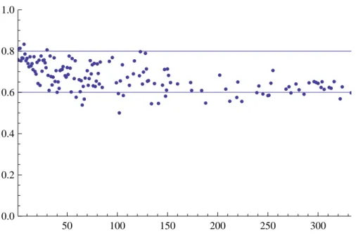
There are many ways to measure the quality of the theoretical predictions with the simulated data. Given that the results of Section V are most central to our motivating questions, we focus on discussing the relationship between degree and individual homophily in the simulated networks.13 In summary, we find strong support for the model’s predictions. Look at Figure 1, which depicts the relationship between individual homophily and degree for a typical simulation. Each point represents the average individual homophily among nodes of a particular in-degree. The bounds from Proposition 11 are depicted as horizontal lines in the the figure. The upper bound is given by h(0) = q+(1−q)(b1+b2−1), and the lower bound is given by limk→∞h(k) = q.
Values cluster very near the upper value for low degree nodes, and appear to asymptote to the lower value, exhibiting a decreasing, convex shape as a function of degree, as predicted.
VI
Empirical analysis
In this section, we study how the predictions of the model compare with empirical properties of social networks. To do so, we analyze the AddHealth data, which contains extensive information
50 100 150 200 250 300 0.0 0.2 0.4 0.6 0.8 1.0
Figure 1: Individual homophily as a function of in-degree for a typical simulation. The
parame-ters here are q = 0.6, b1 = .8, b2 = .7, r = 13 and p = 1. The implied value of γ is approximately 0.86.
on friendship networks in a sample of high schools in the U.S. This data allow us to look at homophily patterns in friendship networks with respect to gender composition. We first describe the data, as it applies to our analysis, in more detail. We then study the relationship between homophily and degree, checking whether the theoretical results of Propositions 10 and 11 hold empirically. Finally, we discuss other empirical properties in light of the model’s predictions. Overall, the theoretical predictions of the model are remarkably well supported by this data.
The analysis below is based on the AddHealth study. We use the first wave of the in-school survey, which was conducted between September 1994 and April 1995 in a representative sample of American high schools. One objective of this survey was to collect information on all students within any particular school. Most relevant from our point of view, students were asked to name their best friends. They could name up to five male friends and five female friends. Friendship nominations are not necessarily reciprocal so these friendship networks are, as such, directed. In what follows, we focus on the in-degree and homophily of a student. A student’s in-degree is defined as the number of other students (in the same school) who name him as one of their best friends. A student’s homophily is the proportion of students with the same gender among
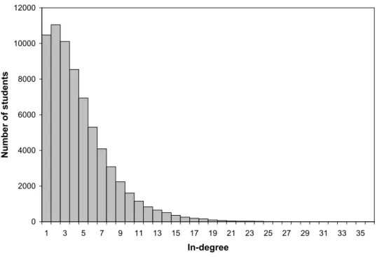
all the students who name him as one of their best friends. It is well-defined only if the student receives at least one nomination. Overall, there are 142 schools and 67,916 students who receive at least one friendship nomination in our sample. The overall proportion of boys is 0.498. Overall network homophily is 0.577 for boys and 0.617 for girls which indicates that, indeed, students are relatively more likely to be friends with others of the same gender.14 Very few links originating in one school of the sample end up in another school. So for our purposes, it is best to view the overall network as the collection of 142 smaller disconnected networks. The identification of our main regression below relies on two sources of variations. First, we have some variation across schools in terms of gender composition. Second, we have natural variation in degrees of students within schools. Figure 2 depicts the frequency distribution of in-degrees in the data.
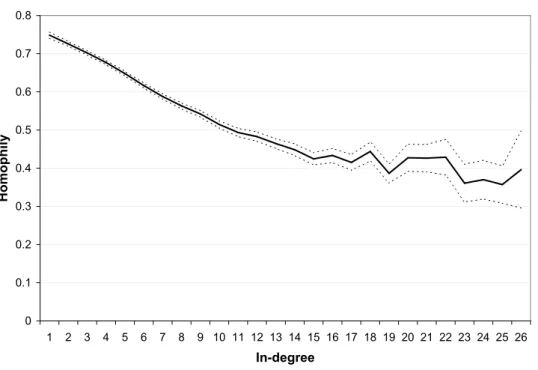
We now look at the relationship between homophily and degree at the individual level. Figure 3 depicts how average individual homophily varies with in-degree over the whole sample.15 The relation clearly shows a decreasing and convex shape. The effect of degree also seems to be qualitatively important. The average individual homophily is equal to 0.748 among students with degree 1, 0.515 among students with degree 10, and 0.427 among students with in-degree 20. Of course, this evidence is only suggestive as the effect of gender composition (q) is not controlled for. To provide a rigorous test of our results, we conduct a set of linear regressions. Denote by hij the individual homophily of student i in school j, by kij the in-degree of student i
in the friendship network of high school j, and by qij the proportion of students in high school j
who have the same gender as i.16 Our analysis in section V shows that under the Location-Bias model individual homophily hij should depend on kij and qij. In particular, the relationship
should be decreasing and convex in kij, increasing in qij and with a positive cross-derivative
between kij and qij. In order to test these hypotheses, we estimate a linear regression of hij on
kij, kij2, qij, and kijqij. We run these regressions over the whole sample as well as separately for
boys and girls. The estimation results are reported in Table 1.
14These figures also indicate a possible asymmetry between boys and girls. However, since these are aggregate
figures, it leaves open the question of whether the asymmetry can be explained by school-level variations. We explore this below.
15Dashed lines represent the 95% confidence interval. 16Thus, if i
1 and i2 have the same gender and are in the same school, qi1j= qi2j and if i1 is a boy and i2is a girl of the same school, qi1j = 1 − qi2j.
0 2000 4000 6000 8000 10000 12000 1 3 5 7 9 11 13 15 17 19 21 23 25 27 29 31 33 35 In-degree N u m b e r o f s tu d e n ts
Figure 2: The distribution of in-degree across students in the AddHealth sample. Whole sample Boys Girls
degree −0.0528 −0.0558 −0.0452 (0.0024) (0.0026) (0.0067) degree2 0.00059 0.00072 0.00058 (4 ∗ 10−5) (6 ∗ 10−5) (6 ∗ 10−5) qj 0.53 0.567 0.268 (0.018) (0.017) (0.087) degree∗qj 0.043 0.048 0.024 (0.004) (0.004) (0.013) Constant 0.512 0.456 0.689 (0.011) (0.012) (0.045) Observations 67916 32876 35040
Table 1. Regression estimates of individual homophily on degree, degree2, q, and an interaction
term degree∗q. Robust standard errors are given in parentheses.
0 0.1 0.2 0.3 0.4 0.5 0.6 0.7 0.8 1 2 3 4 5 6 7 8 9 10 11 12 13 14 15 16 17 18 19 20 21 22 23 24 25 26 In-degree H o m o p h il y
Figure 3: The relationship between individual homophily and in-degree shows a decreasing and
convex pattern.
The first column reports results for the whole sample. Remarkably, all coefficients have the predicted sign and are statistically significant at the 1% level. At q = 0.5, the estimated relationship between homophily and degree is decreasing and convex up through an in-degree of
k = 26, which almost entirely covers the data’s support.17 The effects of q and of kq are also both clearly positive. So holding degree constant, homophily is larger in relatively larger groups. Finally, degree has a lower effect (in absolute value) on homophily in relatively larger groups. The second column reports results for boys only and, likewise, the third column for girls only.
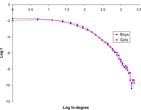
-12 -10 -8 -6 -4 -2 0 0 0.5 1 1.5 2 2.5 3 3.5 Log In-degree L o g f Boys Girls
Figure 4: The pdf of in-degrees for boys (blue) and girls (pink) shown in log-log scale. Again, all the coefficients have the predicted sign. They are also all statistically significant at the 1% level, except for the effect of kq for girls which is statistically significant at the 10% level. At q = 0.5, the predicted relationship between homophily and degree is decreasing and convex for degrees up to k = 21 for boys and k = 28 for girls. The effects of k and k2 are quantitatively similar for boys and girls. However, the effects of q and kq are roughly twice as large for boys than for girls. This indicates some asymmetry between the link formation processes of boys and girls, which is not accounted for in the model.18 In summary, we find strong empirical support for our theoretical predictions relating individual homophily to other network features.
The model yields further testable implications. In section IV, we derive several results con-straining the relationships among various degree distributions. However, the AddHealth data
18There are a number of ways to introduce heterogeneity between the groups beyond their relative sizes. For
consists of a collection of 142 relatively small networks. This prevents an accurate estima-tion of the full degree distribuestima-tions for each network, especially considering that the theoretical predictions rely on a mean-field approximation which becomes valid only for large networks. Still, under the Location-Bias model, F1 should be equal to F2 and should be independent of q (Proposition 8). So the distribution of in-degree for boys should be equal to the distribution of in-degree for girls over the whole sample, provided the other parameters of link formation are fixed throughout the sample. Figure 4 depicts the pdf’s of the two distributions in a log-log plot. While the two distributions are not precisely identical, they are reasonably close.19
Finally, in section III, we show that the relationship between relative homophily and school gender composition should have an inverted-U shape.20 To check for this relationship, we regress
Hj on qj and qj2 over all schools. This yields coefficients that are statistically not significant.21
So the empirical relation between network homophily and gender composition is essentially flat over our sample. Note, however, that empirical values of qj lie mostly between 0.4 and 0.6.22 A
flat relationship between homophily and gender composition around q = 0.5 is consistent with Proposition 8. However, the range is probably too small to lead to an informative test of the result.
VII
Conclusion
In this paper, we develop a parsimonious model of network formation that accounts for group identity and homophily. This is accomplished by introducing type-dependent random meeting biases to the model of Jackson & Rogers (2007). It turns out that doing so enriches the analysis significantly. In particular, we derive sharp theoretical results regarding the specific patterns of homophily in society and the way homophily interplays with other structural
characteris-19The proportion of students with a very low in-degree (0 or 1) is somewhat higher for boys than for girls.
Extending our model to account for such asymmetries, as in footnote 18, provides an interesting direction for future research; see the conclusion.
20Currarini, Jackson and Pin (2008) find empirical evidence of this inverted-U shape on the same data, but
with respect to racial homophily.
21We obtain H
j = 0.053 + 0.479qj− 0.400q2j, with standard errors 0.110, 0.388, and 0.367, respectively. Notice
that the graph of this curve is nearly flat over the range of q observed in the sample.
tics of the network. In particular, we obtain testable implications on the relationship between individual-level homophily, degree and group composition. We test these implications on data from friendship networks between boys and girls in high schools, finding strong empirical support for the model’s predictions. Well-connected students indeed have a more gender-diverse network than those who are relatively isolated.
Our objective is to develop a model that is capable of accommodating rich homophily patterns while keeping the analysis as tractable as possible. One observation that becomes clear is that by introducing a homophilic bias in the very simple way proposed here, the effects on network characteristics can be subtle and complex. However, the analysis has a number of limitations that leave open questions for future research.
First, the link formation process that agents follow is specified exogenously; the incentives that might generate such behavior are not modeled. While non-strategic behavior may be rea-sonable for studying friendships among adolescents, it may not be appropriate in other contexts. We have three comments on this point. First, as shown by Jackson & Rogers (2007), the decision rule can be viewed as a reduced form outcome of an explicit cost-benefit analysis. Their argu-ments can be extended to handle the case of group identities studied here. Second, Campbell (2008) presents a dynamic model of strategic interactions that generates the linking decision of Jackson & Rogers (2007), demonstrating that such a rule can be supported as equilibrium behavior in a fully strategic setting. Third, while the ability to tie network structure back to micro-level incentives is clearly useful, homophilic biases are observed across many settings, and taking this as fact as a primitive of the model, we generate testable implications that are supported in the data.
Second, our analysis handles only the case of two groups. Thus, we can study homophily with respect to any binary characteristic like gender, but not, by direct application of the model, with respect to characteristics that are continuous (e.g. income) or that have several categories (e.g. race). Many of our results and techniques would extend directly to an analysis of an arbitrary (finite) number of groups, however this comes at the cost of the analysis becoming cumbersome
quite quickly.23
Third, in our location-bias model the two groups differ only in terms of their relative propor-tions in the population. As stated, we intentionally introduced group-dependent linking in its simplest form. However, there are various ways to introduce further group heterogeneity into the model, and these have the potential to significantly enhance the analysis. For instance, the two groups could have different values of γ, mr or ms. In principle these effects may be identifiable
empirically as well. Extending the model to account for such asymmetries could help to explain some of the empirical facts presented in Section VI.
Finally, we abstract away from potential biases in the probabilities of initiating a link con-ditional on meeting. In some settings, observed homophily may arise from a bias in interaction opportunities, as in our model, or instead from a bias in preferences. That is, one could consider a model in which the probability of connecting to an agent depends on whether or not the two individuals belong to the same group, thereby introducing a second group-dependent bias. Our model allows us to provide a clean analysis of how homophily and network formation are affected by biases in the meeting process only. Examining the data, the analysis shows that empirical patterns of homophily may be well explained by such opportunity bias. Still, both types of biases may matter in other contexts. Empirically identifiying the precise source of homophily is an important question. A promising direction for future work is to account for both types of biases in a common framework, to study their interaction and their joint empirical implications.
23For instance, to derive the analog of Proposition 4 with G groups, we have to solve a system of G differential
APPENDIX
Consider a degree distribution F (k) obtained implicitly through a process such that ki(t) =
f (t/i) and another degree distribution G such that ki(t) = g(t/i), with ki(i) = 0. Assume f and
g are weakly increasing and continuous on [1, +∞[ and that limx→∞f (x) = limx→∞g(x) = ∞.
Lemma 1 F First-Order Stochastically Dominates G if and only if for all x ≥ 1, f (x) ≥ g(x),
with strict inequality for some x.
Proof. Assume f (x) ≥ g(x) for all x ≥ 1. Pick k and t arbitrarily. Define if as the birthdate of
the node with degree k at time t under f , and similarly for ig. We have f (t/if) = k ≥ g(t/if),
which, since g is non-decreasing implies that ig ≤ if. Since Ft(k) = 1−if/t and Gt(k) = 1−ig/t,
we have Ft(k) ≤ Gt(k).
Now take ¯x such that f (¯x) > g(¯x). Pick k and t arbitrarily. Define if = t/¯x and ¯k to be the
size of node if at time t under f . Then set ig to be the node with degree ¯k at time t under g.
We have ¯k = f (t/if) = f (¯x) > g(¯x) = g(t/if), which implies that ig < if. Thus Ft(¯k) < Gt(¯k).
To show necessity, fix t and choose if so that f (t/if) < g(t/if), and set ¯k = f (t/if).
Defin-ing ig as the node with degree ¯k at time t under f , we know that ig > if. This implies that
Gt(¯k) < Ft(¯k), completing the proof.
Proof. Proposition 4 Setting k = k11 k12
, in vector notation, the system of equations to solve is
˙k = 1
tA +
1
with A = m1+rr b1 m r 1+r(1 − b2) 1−q q B = 1 mr(1 + r) b1mr 1−qq (1 − b1)mr 1−q q (1 − b2)mr brmr ≡ 1 mr(1 + r) B0
In order to solve equations (VII.3), we transform the system by diagonalizing B. To that end we compute the eigenvalues of B0, by writing
det(B0− λI) = λ2− mr(b1+ b2)λ + m2r(b1b2− (1 − b1)(1 − b2)),
which has solutions
λ0 = mr 2 ³ (b1+ b2) ± p (b1+ b2)2+ 4[b1b2− (1 − b1)(1 − b2)] ´ = mr 2 (b1+ b2± (b1+ b2− 2)) ,
which are non-negative if and only if b1 + b2 ≥ 1. Let λ1 and λ2 be the eigenvalues of B, i.e., the solutions just computed scaled by 1
mr(1+r), which gives λ1 = 1 1+r and λ2 = b1+b2−1 1+r ; set Λ = λ1 0 0 λ2
. Then, there exists a matrix P such that B = P−1ΛP . Introduce x = P k.
Multiplying equation (VII.3) by P leads to ˙x = 1
tP A +
1
tΛx
Recall, the solution of ˙y = a t +
by
t with y(i) = 0 is y(t) = ab((ti)b − 1). The initial conditions are
x(i) = (0, 0)0 since k(i) = (0, 0)0. This yields
x1 = (P A)1 λ1 [(t i) λ1 − 1] x2 = (P A)2 λ2 [(t i) λ2 − 1],