HAL Id: hal-01582936
https://hal.archives-ouvertes.fr/hal-01582936
Submitted on 9 Sep 2019
HAL is a multi-disciplinary open access
archive for the deposit and dissemination of
sci-entific research documents, whether they are
pub-lished or not. The documents may come from
teaching and research institutions in France or
abroad, or from public or private research centers.
L’archive ouverte pluridisciplinaire HAL, est
destinée au dépôt et à la diffusion de documents
scientifiques de niveau recherche, publiés ou non,
émanant des établissements d’enseignement et de
recherche français ou étrangers, des laboratoires
publics ou privés.
Green energy aware scheduling problem in virtualized
datacenters
Gilles Madi Wamba, Yunbo Li, Anne-Cécile Orgerie, Nicolas Beldiceanu,
Jean-Marc Menaud
To cite this version:
Gilles Madi Wamba, Yunbo Li, Anne-Cécile Orgerie, Nicolas Beldiceanu, Jean-Marc Menaud. Green
energy aware scheduling problem in virtualized datacenters. ICPADS 2017 : IEEE 23rd International
Conference on Parallel and Distributed Systems, Dec 2017, Shenzen, China. pp.648-655,
�10.1109/IC-PADS.2017.00089�. �hal-01582936�
Green energy aware scheduling problem
in virtualized datacenters
Gilles Madi-Wamba
∗, Yunbo Li
∗†, Anne-C´ecile Orgerie
†, Nicolas Beldiceanu
∗and Jean-Marc Menaud
∗∗IMT Atlantique, LS2N, Nantes, France – Email: {gmadiw14, nicolas.beldiceanu, jean-marc.menaud}@imt-atlantique.fr †CNRS, IRISA, Rennes, France – Email: {yunbo.li, anne-cecile.orgerie}@irisa.fr
Abstract—With the generalization of cloud infrastructures usage, energy consumption has become a major issue. Scheduling heuristics have been proposed to optimize the resource usage of data center so as to take down the energy consumption. This paper tackles the problem with a different approach by taking into consideration the availability of renewable energy. First we formalize the green energy aware scheduling problem (GEASP) and propose a global model based on constraint programming as well as a search heuristic to solve it efficiently. The proposed model integrates the various aspects inherent to the dynamic planning in a data center: heterogeneous physical machines, various application types (i.e., active or online applications and batch applications), actions and energetic costs of turning ON/OFF physical machines, interrupting/resuming batch appli-cations, CPU and RAM resource consumption, tasks migration, migration costs, and integration of green energy availability. The model can therefore reduce both the costs related to energy consumption and the carbon footprint of a data center. We evaluate the model against the state-of-the-art framework PIKA on real-world workload and solar power traces.
I. INTRODUCTION AND RELATED WORK
Over the years, energy consumption has become a major concern in the field of information technologies. Amazon reports that the cost related to the energy consumption over a 3-years period is more than 40% of the overall cost of its data center [11]. Besides, in [3], Barrosso shows that over the lifetime of a data center, the expenses related to the energy consumption can easily surpass the hardware cost. In the literature, most work that attempts to reduce the energetic cost of a data center proceeds by reducing the overall energy consumption [9], [8]. Apart from the economic aspect, massive energy consumption also has repercussion on the environment, as the brown energy is produced from polluting sources. In this paper, we propose not only to reduce the brown energy consumption to handle the economic issue, but also to maximize green energy consumption to take care of the environmental issue.
The energy consumption of a system comprises a static and a dynamic part [16]. The static part is linked to the system size and the hardware type, and the dynamic part is linked to resources usage. In [15] and [6], Li et al. propose a novel framework, oPportunistic schedullIng broKer infrAstructure (PIKA) that aims at reducing the brown energy consumption of a small/medium-size data center. According to the amount of green energy available at each time slot PIKA turns physical machines ON/OFF, pauses, resumes or migrates jobs. However, this opportunistic scheduling is rather reactive than
proactive. In this paper, we first formalize the green energy aware scheduling problem (GEASP). Second, we propose a global constraint programming model as well as a search heuristic and show that our model can significantly optimize the overall energy consumption of a data center. The proposed model simultaneously takes into account each of the following aspects:
• compatibility with both active and batch applica-tion types,
• applications resources requirements varying over the time,
• migration of applica-tions from one physical server to another,
• energetic cost of
appli-cation migrations,
• interruption/resumption
of batch applications,
• compatibility with he-terogeneous physical servers i.e. the resources are variable from one physical server to an-other,
• turning ON/OFF the physical servers and resources management,
• extra energy
consump-tion to turn a physical server ON/OFF,
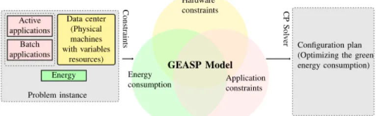
• green energy integration. The main advantages of constraints programming include a certain level of flexibility that PIKA lacks. Indeed, thanks to this feature, the proposed model is also compatible with business constraints inherent to data center infrastructure man-agement as well as with user preferences. Figure 1 illustrates different aspects of this context.
Data center (Physical machines with variables resources) Active applications Batch applications Energy Problem instance Constraints CP Solv er Hardware constraints Energy
consumption Applicationconstraints
GEASP Model
Configuration plan (Optimizing the green energy consumption)
Fig. 1: The GEASP model computes a global and pro-active configuration plan that minimizes the brown energy and max-imizes the green energy consumption of the data center while satisfying all the constraints. Hardware constraints are related to memory/CPU limitations and turning the servers ON and OFF. The application constraints are related to the interruption, the migration, and the placement of the applications as well as to some business constraints (ban, lonely, spread, . . . ).
The rest of the paper is organized as follows: Section II describes the problem and gives all the necessary definitions and Section III formalizes the GEASP problem and presents our model. In Section IV, we present the search heuristic to find suitable solutions to the GEASP. Finally, we evaluate our contribution using real data center workloads and green energy traces in Section V, and we conclude in Section VI.
II. PROBLEM DESCRIPTION AND DEFINITIONS
We consider the problem of scheduling in a small/medium size data center with limited resources [5]. The scheduling should minimize the brown energy consumption and maximize the green energy consumption. We recall that a data center is made up of one or more servers that host the applications. We have two types of applications, the active and the batch. Both types of application are introduced in Section II-A.
A. Definitions
Active Application An active application is an application that is executed throughout the time horizon without being interrupted. Each active application is described by its:
• Memory consumption, i.e. is the constant amount of RAM consumed by the application within the server it is hosted.
• CPU Usage, the processing power used by a server to execute the application; it may vary from one time slot to the next throughout the horizon.
• Migration cost, i.e. the extra energy consumption needed to migrate an application from one server to another. An active application ai of memory requirement memi,
CPU usage cpui and migration cost migri is denoted
ai(memi, cpui, migri).
Batch Application A batch application or batch job is an application that can be interrupted and resumed. A time slot during which a batch job is running is called a runtime. Each batch application is characterized by its :
• Memory consumption: its memory consumption of a batch job is constant.
• CPU Usage: CPU usage of a batch job is constant. • Duration.
• Migration cost.
• Slack. The total amount of time during which it is interrupted shall not exceed a given slack.
A batch job bi of memory memi, CPU usage cpui,
du-ration di, migration cost migri and slack si is denoted
bi(memi, cpui, di, migri, si).
Server We define a server in this problem as a machine that hosts the applications. It is characterized by:
• its Memory limit is the total amount of memory that is shared among the hosted applications.
• its CPU limit is the total amount of processing power that can be shared among hosted applications.
• its ON (resp. OFF) energy is the constant amount of energy required to turn the server ON (resp. OFF).
• its load/consumption relation, which relates the CPU load of the server to its energy consumption.
• its id is a unique integer that identifies each server. A server i of memory MEMi, CPU limit CPUi, ON energy
Eoni, OFF energy Eoffi, load/consumption relation r and id
idi is denoted si(MEMi, CPUi, Eoni, Eoffi, ri, idi).
Our goal is to compute an energy efficient configuration plan for the data center which, while reducing the amount of brown energy used and increasing the proportion of green energy, copes with the operational and the business constraints of different application types. Next definition introduces the notion of Configuration plan.
Configuration plan Given a time horizon, a set of active and batch applications and a data center, a configuration plan is a scheduling that meets the following requirements:
• At any time slot through out the horizon, it specifies for each active application an allocated server. A migration occurs when the host of an active application changes from one time slot to the next.
• It specifies when each batch job starts, when it ends, and eventual interruption and resumption times. For any batch job, the configuration plan specifies the hosting server at any timepoint. A migration occurs when the host changes from one time slot to the next.
• For each server of the data center, it specifies every time slot when the server is turned ON or OFF.
The configuration plan is energy efficient when it maximizes the green energy consumption of the data center. Indeed, the availability of green energy fluctuates over the time. Typical example is the solar energy.
Section III formalizes this problem into a constraint model. III. MODEL OF THE PROBLEM
In this section, we propose a constraint based model to capture the already mentioned aspects of the green energy aware scheduling problem in virtualized data centers. Before detailing different parts of the model, we first shortly recall key notions of constraint programming in the context of virtualized data centers.
A. Background on constraint satisfaction problems
Constraint satisfaction problem A constraint satisfaction problem (CSP) [17] is a triple P = (X, D, C) where :
• X is an tuple of n > 0 variables, X = hx0, x1, . . . , xn−1i.
• D is a tuple of n > 0 domains, D = hD0, D1, . . . , Dn−1i
such that xi∈ Di.
• C is a tuple of k > 0 constraints C = hC0, C1, ..., Ck−1i.
We now define the notion of constraint.
Constrain Given a CSP P = (X, D, C), a constraint Ci∈ C
is a pair hRi, Sii where Si is a subset of X, and Ri is a
relation over Si. The relation Rispecifies the tuples of values
forbidden among the Cartesian product of the domains of the variables in Si.
Solution of a CSP Given a CSP P = (X, D, C), a solution S of P is a tuple hv0, v1, ..., vni such that vi ∈ Di and for
every constraint Ci= hRi, Sii ∈ C, the relation Ri holds.
B. Constraint programming for the green energy aware scheduling problem in virtualized data center
Constraint programming is a suitable solution to solve most scheduling problems [2]. In the case of a green energy aware scheduling problem, constraint programming is well suited as it has a good expressiveness to precisely model each component of the problem. It also enables to add any new constraint to an existing model. In [13], Hermenier et al. present four side constraints that may be required by the administrator of a system or by the users to restrict the placement of the applications into servers.
• Ban. At a given time t, the system administrator may want to turn off a server to perform a hardware or a software maintenance.
• Spread. In order to achieve tolerance to hardware fail-ures, an application may use replication. For the fault tolerance, the application and its replication should run at any time on different servers.
• Lonely. For some reasons, an application may require to run alone in a server.
• Capacity. Sometimes, due to some shared resources, it might be useful to limit the number of applications executed in a server. The capacity constraint is used to ensure that the number of applications hosted on a given server is below a given limit.
This list of side constraints is not exhaustive. Besides the good expressiveness and the flexibility, the solving process of a constraint satisfaction problem through constraint propa-gation [17] ensures that all the constraints of the problem are satisfied.
We now formalize the definition of a green energy aware scheduling problem.
Green energy aware scheduling problem A green energy aware scheduling problem (GEASP) is a tuple such that P = {S, A, B, T, E} where:
• S is a set of servers.
• A is a set of active applications. • B is a set of batch jobs.
• T is the time horizon: an integer specifying the total number of time slots to consider.
• E is a time series of length T which specifies the quantity of green energy available at each time slot.
In Sections III-C up to III-G, we present how we formalize each aspect of a GEASP into a constraint satisfaction problem. We will use the toy example III.1 to illustrate our model. Example III.1. Throughout this paper, we use the following toy GEASP. P = {S, A, B, T, E} where:
• S = {s0(3, 50, 3, 3, r, 0), s1(3, 50, 3, 3, r, 0)} where we
have r(cpu load) = 10 + cpu load
• A = {ao(1, 20, 2)}
• B = {b0(2, 20, 3, 1, 5), b1(2, 20, 3, 1, 5)} • T = 10h
• E = 10, 10, 10, 90, 90, 10, 10, 10, 48, 43
An energy efficient configuration for the GEASP is given below:
• Slot 0 s0 is turned ON,
and a0 is placed on s0. • Slot 1 No change. • Slot 2 No change. • Slot 3 b0 is launched on s0. s1 is turned ON and b1 is launched on it. • Slot 4 No change.
• Slot 5 b0 and b1 are
interrupted and s1 is turned OFF. • Slot 6 No change. • Slot 7 No change. • Slot 8 b0 is resumed on s0.
• Slot 9 b1is resumed and
migrated from s1 to s0.
C. Turning a server ON or OFF
To model the action of turning a server ON and OFF, we have to consider two aspects. First we need to consider the inherent energetic costs of these actions, and second we need to ensure that no application can be scheduled on a switched off server.
1) Energetic cost: As seen in the definition of a server in Section II-A, each server has a turning ON/OFF cost. Let P = {S, A, B, T, E} be a GEASP. For each server Si(MEMi, CPUi, Eoni, Eoffi, ri, idi) ∈ S, a set of T + 1
boolean variables ON(i,t) indicate at each time slot t(t ∈
[−1, T − 1]) if the server is ON or OFF. ON(i,−1) = false
indicates that server Si is initially off.
Turning a server ON or OFF at a time slot t con-sumes an extra energy at this time t. For each server Si(MEMi, CPUi, Eoni, Eoffi, ri, idi), the model of this
en-ergetic cost relies on T switch task variables. Before we detail these variables, we first introduce the notion of task.
Task A task i is a tuple taski(si, di, ei, < ri >, hi) where:
• si is the start time of the task.
• di is the duration of the task.
• ei is the end of the task.
• < ri > is the list that contains all the resource
require-ments of the task. A task might consume one or more resources of different types.
• h is the server hosting the task.
Given a server si(MEMi, CPUi, Eoni, Eoffi, ri, idi), the
energy consumption of its switch task at time t depends of the server si being turned ON or OFF at that time t. It is a
variable switch energyi,t given by :
switch energyi,t= Eoni∗ (ON(i,t−1)< ON(i,t)
+ Eof fi∗ (ON(i,t−1)> ON(i,t)). (1)
where a term like ON(i,t−1) > ON(i,t) is interpreted as a
0 − 1 variable that will be assigned value 1 (resp. 0) if the corresponding conditions holds (resp. doesn’t hold).
Example III.2. According to the configuration plan given in Example III.1 we have:
• switch energy0,0 = 3 Since server s0 is turned ON at
t = 0.
• switch energy1,3 = 3 Since server s1 is turned ON at
t = 3.
• switch energy1,5= 3 Since server s1 is turned OFF at
t = 5.
• switch energy0,t = 0 for all t 6= 0 and besides
switch energy1,t= 0 for all t ∈ {0, 1, 2, 4, 6, 7, 8, 9}
2) Availability of a server: The availability of a server is the constraint that makes a server unavailable for scheduling at any time slot during which it is switched off. Since any application consumes a strictly positive amount of memory on the server on which it runs, a server can not host any application if it has no free memory available. Thus to make a server unavailable, we set its available memory to 0. To do so, we create memory tasks whose aim is to fill any server’s memory at any time t when the server is off.
In order to avoid creating T extra tasks, we add a memory resource memi,t to the switch tasks of Section III-C1. The
memory consumption mi,t of the switch task switch(i,t) of
a server si(M EMi, CP Ui, Eoni, Eof fi, ri, idi) at time t is
given by :
memi,t = M EMi∗ (ON(i,t)= 0). (2)
The switch tasks of the model are therefore indexed by the server index i and the time slot t, they are denoted switch(i,t)(t, 1, t + 1, < energyi,t, memi,t>, i).
Section III-D here after describes how we model active and batch applications using the notion of task introduced in Definition III-C1.
D. Modeling the applications
The most difficult part of a GEASP is the model of the applications. The model should take into consideration the following requirements:
• [Host]. At any time t any active application and any uninterrupted batch job should be hosted on a server. • [Migration]. Both active and batch applications can be
migrated from one server to another one. These migra-tions have costs that should be taken into consideration. Details on how to model the migration costs are given in Section III-E.
• Active applications are never interrupted.
• Batch jobs can be interrupted as long as the corresponding slack constraint is not violated.
In order to meet these requirements, we model each active application ai(memi, cpui, migri) (resp. each batch
appli-cation bi(memi, cpui, di, migri, si)) by a set Sai (resp. Sbi)
of tasks.
1) Active applications: As active applications are not interrupted, each active application ai(memi, cpui, migri)
is modeled by a set Sai of T tasks that are denoted
sub(ai,t)(t, 1, t + 1, < memi,t, cpui,t, energyi,t>, hi,t), t
from 0 to T − 1 where:
• memi,t (resp. cpui,t) is the memory consumption (resp.
the CPU usage) of the task ai(memi, cpui, migri) at
time t.
• hi,t is the server that hosts ai(memi, cpui, migri) at
time t.
• energyi,tis the amount of extra energy consumed by the
server hi,t to host sub(ai,t).
2) Batch applications: Since the duration of each batch job is fixed, any batch job bi(memi, cpui, di, migri, si)
is modeled by a set Sbi of di tasks which are denoted
sub(bi,j)(s(bi,j), 1, e(bi,j), < memi,j, cpui,j, energyi,j>, hi,j)
where j ∈ [0, di− 1].
The batch applications can be interrupted and resumed. Therefore s(bi,j) and e(bi,j) are variables taking values in
[0, T − 1] with the following constraints:
∀j ∈ [1, di− 1], s(bi,j)≤ e(bi,j−1) (3)
The slack constraint is modeled as follows:
e(bi,di−1)− s(bi,0)− di ≤ slack. (4)
For both active and batch jobs, the variables energyi,t and
energyi,jspecify how much extra energy is needed by a server
to host this given application. Its value varies from one host to another. Details on how this value is set are presented in Section III-G.
To ensure that a server s in which a task is scheduled at time t is ON at that time, we add the following constraint for each active and batch tasks.
∀sub(ai,t)(t, 1, t+1, < memi,t, cpui,t, energyi,t>, hi,t) ∈ Sai,
hi,t= s ⇒ ON(s,t)= 1 (5)
∀sub(bi,j)(j, 1, j+1, < memi,j, cpui,j, energyi,j>, hi,j) ∈ Sbi,
hi,j= s ⇒ ON(s,t)= 1 (6)
E. Migration cost
This section models the migration cost of both active and batch applications. For any active application ai(memi, cpui, migri) and any task
sub(ai,t)(t, 1, t + 1, < memi,t, cpui,t, energyi,t>, h(i,t)) ∈
Sai, we create a migration task
migr(ai,t)(t, 1, t + 1, < migr energyi,t>, h(i,t)) where
migr energyi,tis the energy that is consumed whenever this
active task ai is migrated from one server to another at time
t. Its value is given by: migr energyi,t =
(
0 t = 0
migri∗ (h(i,t)6= h(i,t−1)) t > 0
Similarly, we create migration tasks migr(bi,j) for batch
applications.
Example III.3. According to the configuration plan given in Example III.1, we have:
• migr energyb1,9 = 1 since batch application b1 is
F. Memory consumption and CPU usage
Each server has a limited quantity of memory and CPU. An application can be scheduled on a server si∈ S at time t if and
only if server sihas enough resources to satisfy the application
requirements. To take these constraints into consideration, we use a cumulative constraint [1], [14].
Cumulative constraint Given a set T of single resource tasks, the cumulative constraint ensures that at any time t, the cumulative resource of the set of tasks scheduled at t does not exceed a fixed limit.
The standard definition of the cumulative constraint given above assumes that there is one single host for the tasks. We will instead use the cumulatives constraint [4], a slightly generalized version of the cumulative constraint which allows more than one host, i.e. more than one server. The cumulatives constraint:
cumulatives(Tasks,Machines) where
• T asks is a set of single resource tasks of the form task(start, duration, end, resource, host).
• M achines is a set of fixed resource hosts of the form machine(id, resource limit).
holds if, for each machine m, at each point t, where at least one task is assigned to machine m, the cumulative resource of the set of tasks assigned to m at t is less than or equal to (respectively greater than or equal to) the capacity associated with machine m.
The host of a task is the id of the server where it is sched-uled. Before we detail the use of the cumulatives constraint in the case of memory and CPU usage, we first introduce the notion of restriction of a task to a given resource.
Restriction of a task Given a task t(start, duration, end, < r1, r2, . . . rn >, host) its restriction to the resource r ∈<
r1, r2, . . . rn > is the task t r(start, duration, end, r, host).
To model the memory consumption and CPU usage of a GEASP, we will use two cumulatives constraint, cumulatives(M emory T asks, M emory M achines) and cumulatives(CP U T asks, CP U M achines) where:
• M emory T asks is the set of active tasks, batch tasks and switch tasks restricted to the memory resource. • CP U T asks is the set of active tasks, batch tasks and
switch tasks restricted to the CPU resource plus a set of complementary tasks that we use to compute the energy consumption of each server at each time slot. Details on these complementary tasks are given in Section III-G. • M emory M achines and CP U M achines are the set
of machines built in the following way:
1 M emory M achines = {machine mem(idi, M EMi) such that
∃si(M EMi, CP Ui, Eoni, Eof fi, ri, idi) ∈ S}
2 CP U M achines =
{machine cpu(idi, CP Ui) such that
∃si(M EMi, CP Ui, Eoni, Eof fi, ri, idi) ∈ S}
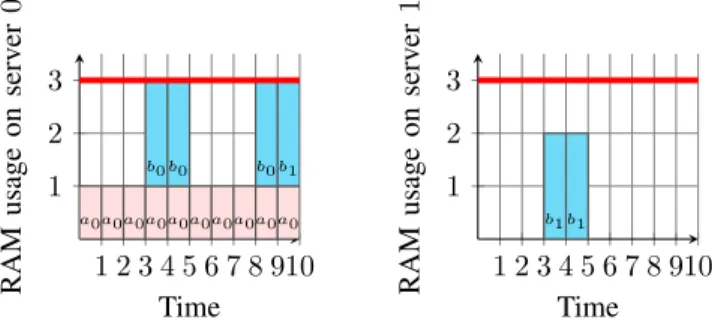
Example III.4. Figure 2 shows how the cumulatives constraint takes into consideration the RAM limit of each server at each time slot in the configuration plan given in Example III.1.
1 2 3 4 5 6 7 8 910 1 2 3 a0a0a0a0a0a0a0a0a0a0 b0 b0 b0 b1 Time RAM usage on serv er 0 1 2 3 4 5 6 7 8 910 1 2 3 b1 b1 Time RAM usage on serv er 1
Fig. 2: cumulatives constraint for the RAM resource limits
G. Minimizing the brown energy consumption
Before we detail how to minimize the brown energy con-sumption of a data center, we first need to specify how to compute the energy consumption of a server. We assume server si is already turned ON at time t ∈ [0, T − 1] and there is no
migration scheduled at time t. Then the energy consumption ei,t of si at time t is obtained from Equation (7) by:
ei,t = r(loadsi,t) (7)
where loadsi,t is the CPU load in percent of
si at time t. Therefore to know the energy
consumption of a given active (resp. batch) task sub(ai,t)(t, 1, t + 1, < memi,t, cpui,t, energyi,t>, hi,t)
(resp. subt,1,t+1,<memi,j,cpui,j,energyi,j>,hi,j)) at time t, we
first need to know the CPU capacity of the host hi,t (resp.
hi,j) in which it is scheduled at time t. The problem is that
hi,t (resp. hi,j) is not initially fixed, so we have no way to
know in advance the CPU capacity of the host. To overcome this issue, we introduce the element constraint [18]. element constraint Given a list L of integer values, two integer variables index and V , the element (L, index , V ) constraint ensures that V is the indexth element of L i.e
V = Lindex.
Let CP U Capacities be the list of the CPU capacities of the servers. The list is sorted in ascending order of servers id’s. For any time t ∈ [0, T −1] and for any active (resp. batch) task sub(ai,t)(t, 1, t + 1, < memi,t, cpui,t, energyi,t>, hi,t)
(resp. sub(bj,j)(s(bi,j), 1, e(bi,j), < memi,j, cpui,j, energyi,j
>, hi,j)) we state:
element(h, CP U Capacities, HostCapacity) (8) The energy consumption energy of the task is therefore given by:
energy = r( cpu ∗ 100
We now present the energetic model that we used in this paper to characterize the function r for all the servers.
Energetic model: As seen in Section II-A, each server is characterized by a relation r that relates its workload to its energy consumption. In [15], Li et al. experimented multiple tests on Taurus node at the Lyon site of Grid’5000, a large-scale and versatile test-bed for experiment driven research. Each node has 12 cores and each core presents 8.3% overall CPU utilization. They came out with the conclusion that, the overall energy consumption of the node depends on the number of activated cores. Table I summarizes these results.
# cores 0 1 2 3 4 5 6
Power (W) 97 128 150 158 165 171 177
# cores 7 8 9 10 11 12
Power (W) 185 195 200 204 212 220
TABLE I: Experimental energy consumption of a 12 cores node according to the number of activated cores
Following the idea of the PowerModel of CloudSim [7], we use Table I to implement the function getPower() in order to compute the energy consumption of a server. The pseudo code of getPower() is given in Algorithm 1. We thus have :
energy(h, t) = r(load(h, t)) = getP ower(CP Uh, cpu usedh,t)
(10) where CP Uh is the CPU capacity of host h and
cpu usedh,t is the amount of CPU used in host h at time
t.
Algorithm 1 Procedure getPower() to compute the energy consumption of a server according to its CPU load
Require: CPU Capacity . The CPU capacity of the server Require: CPU Used . CPU usage of the server P ower table ← [97, 128, 150, 158, 165, 171, 177, 185, 195, 200, 204, 212, 220] Step ← 1 12× CP U Capacity A ← 1 Step+1× CP U U sed B ← min(A + 1, 13) EA← P ower tableA EB ← P ower tableB
Energy ← EA + ((EB − EA) × CP U U sed ×
10)/(CP U Capacity × 10) return Energy
The value energy(h, t) only takes into consideration the load of the host h. To obtain the actual consumption of the data center, we need to take into consideration all the extra energy costs resulting from turning the servers ON and OFF, and migrating the tasks over the different hosts.
Equation 11 states the total energy consumption of the data center at a given time slot t.
Et= X h energy(h, t) +X a migr energy(ai,t) +X b migr energy(bi,t)+ X h,t switch energy(h,t) (11) where:
• migr energy(ai,t)(resp. migr energy(bi,t)) is the extra
energy consumed at time t whenever the active task a (respectively batch task b) is migrated from one host to another at time t.
• switch energy(h,t) is the extra energy consumed at time
t when host h is switched ON or OFF at time t. Equation 12 computes the total amount of brown energy consumed by the data center at time t.
Bt= max(0, Et− Gt) (12)
where Gt is the amount of green energy available at time
slot t. Finally, Equation 13 computes the total amount of brown energy consumed by the data center throughout the time horizon. B = T −1 X t=0 Bt (13)
Example III.5. Figure 3 shows the overall energy con-sumption of the data center with the configuration plan of Example III.1. As we can see from the plot, the batch jobs are run, migration are executed, and servers are turned ON preferably during time slots when the green energy is highly available. This is achieved by our heuristic that we present in Section IV. 1 2 3 4 5 6 7 8 9 10 10 20 30 40 50 60 70 80 90 S0 S0 S0 S0 S0 S0 S0 S0 S0 S0 S1 S1 S1 M B1 A0 A0 A0 A0 A0 A0 A0 A0 A0 A0 B0 B0 B0 B1 B1 B1 Time Ener gy consumption
Fig. 3: Energy consumption of the configuration plan. The red curve is the green energy availability per slot
An energy efficient configuration plan is one that minimizes the total amount of brown energy B consumed by the data center throughout the horizon. Thus the overall objective of the GEASP is to minimize B.
IV. SOLVING THEGEASP
According to the problem size, it might take a long time to find an optimal solution to a constraint satisfaction problem and to prove its optimality. To overcome this issue, it is important to have a dedicated search strategy that speeds up the process of finding a good solution.
We propose a dynamic heuristic that targets the starts of the batch tasks. Once these variables are fixed, the other variables of the problem will be fixed by propagation.
Since the batch tasks are the ones whose start and end variables are flexible, the intuition of the heuristic is to try to schedule them at times when the green energy is highly available. To do so, we proceed as follows.
1) Variables ordering: Let b(mem, cpu, d, migr, slack) be a batch application modeled by the set Sbof batch tasks of the
form sub(b,i)(s(b,i), 1, e(b,i), < mem, cpu, energy >, h). The
order in which the start variables of the batch tasks in Sb are
fixed is s(b,0), s(b,1), . . . , s(b,d−1). The purpose of this order
is to take into consideration the precedence constraint stated in Equation 3 through out the search.
2) Values ordering: This part of the search strategies deals with the order in which values are chosen from the domain of each start variable. Let s(b,i) be the start of sub(b,i). We
have dom(s(b,i)) = [0, T − 1]. Following the intuition, the
idea is to try to fix s(b,i) to a value t ∈ dom(s(b,i)) when the
green energy availability is maximal. Doing this ensures that we maximize the green energy consumption. We proceed in two steps:
1 Sort step. This is the first step that is performed each time a start variable has to be instantiated. Let E = e0e1. . . eT −1 be the green energy of a
GEASP where E(t) = et, t ∈ [0, T − 1] is the
amount of green energy available at time t. We sort the values et in descending order and obtain the list
SortedE = e(0,t0), e(1,t1), . . . , e(T −1,tT −1) such that
∀e(i,ti)∈ SortedE, E(ti) = eti = e(i,ti)
This gives the order in which values are chosen from dom(s(b,i)), namely t0, t1, . . . , tT −1.
2 Update step. This step is performed immediately after a start variable is fixed. Let a batch task sub(b,i)(s(b,i), 1, e(b,i), < mem, cpu, energy >, h) and
suppose s(b,i) is fixed to t ∈ [0, T − 1]. Since running
sub(b,i) consumes energy, this step updates the green
energy available at time t. This update is done by decrementing E(t) by energy. The following constraint updates the green energy.
E ← e0, e1, . . . , et− energy, et+1, . . . , eT −1 (14)
The Sort step and the Update step presented in this Section sketch the general idea of the heuristic to solve the GEASP. It is possible to optimize the Sort step by avoiding a total sorting over all the indices. The advantage of doing a partial sort is that, since some tasks are linked through a precedence relation, it does not delay too much the first tasks of the precedence chain.
V. EVALUATION
To measure how effective is the model when used in a small/medium size data center, we run simulations on real workload traces.
As stated in [6], finding real traces for data center’s activity is very difficult. For this, we studied anonymized traces provided by EasyVirt, a French SME monitoring Cloud data centers. We used 3 real workload data sets. Each data set reports the activity of a Cloud provider with 55 servers over a 12 hours period. The traces reports client requests for virtual machines with specified CPU and RAM needs. In the context of a virtualized data center, the virtual machines are used to encapsulate the applications that are executed on the physical machines. Before we present the results of the evaluation, we first give details on the used data set.
Data set description
Each of the 3 real workload data set is organized as follows: (1) We have 55 servers, where each server is characterized
by a limited amount of CPU and RAM resource. (2) A set of 567 active applications to be encapsulated
into virtual machines. As introduced in section III-D, each active application is executed throughout the time horizon. In our case, the time horizon is 12 hours. We see from the traces that the CP U and RAM needs of an active application may vary from one time slot to another. This translates into 6804 = 567 × 12 active tasks to handle. The migration cost in terms of energy consumption is also specified.
(3) A set of 2268 batch applications to be encapsulated into virtual machines. Each batch application has a fixed execution time, a slack value, a fixed start time and a migration cost. The requirements of the batch applications also vary from one time slot to another. This translates into more than 6500 batch tasks to handle.
(4) The renewable energy availability. Each data set includes a time series of length 12. This time series is the record of the renewable energy available every hour.
To evaluate our model and to follow the same protocol as in [15], we compared the results to those of a baseline first fit algorithm. The first fit algorithm tries to schedule the task as soon as possible when there is enough resources available. Both models were implemented in Prolog with the constraint solver Sicstus Prolog [10].
Figures 4a and 4b show how the model is able to move a considerable amount of the data center workload to slots where green energy is available.
0 1 2 3 4 5 6 7 8 9 10 11 12 0 0.5 1 1.5 2·10 5 Time axis Ener gy (W atts) Green energy Data center workload
(a) Baseline 0 1 2 3 4 5 6 7 8 9 10 11 12 0 0.5 1 1.5 2·10 5 Time axis Ener gy (W atts) Green energy Data center workload
(b) GEASP Fig. 4: Workload scheduling.
Total E.C Brown E.C. Green E.C
Baseline 78811 39019 39792
GEASP Model 78694 18500 60194
-0.14% -52.58% +51.27%
TABLE II: Energy saving on the first real trace (W).
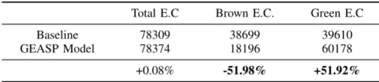
Total E.C Brown E.C. Green E.C
Baseline 78309 38699 39610
GEASP Model 78374 18196 60178
+0.08% -51.98% +51.92%
TABLE III: Energy saving on the second real trace (W).
Tables II, III and IV give details on how the GEASP model significantly reduces the brown energy consumption and increases the green energy consumption.
Total E.C Brown E.C. Green E.C
Baseline 79100 36195 42905
GEASP Model 78868 14670 64198
-0.29% -59.46% +49.62%
TABLE IV: Energy saving on the third real trace (W). On average compared to baseline, GEASP model reduces by 55% the brown energy consumption of the data center and increases by 50.9% its green energy consumption. Although PIKA [15] has a much higher green energy consumption as compared to the baseline algorithm, it does so with two major drawbacks. First, unlike PIKA [15] that uses opportunistic scheduling, our model finishes all the tasks not later than the baseline. This advantage comes from the time horizon that is fixed such that no task is allowed to be scheduled beyond it. If the time horizon constraint is dropped, then there will eventually be room for more optimization. For example, an amount of the workload at slot 11 of Figure 4b could be opportunistically postponed to a later slot where there is more green energy available. But this in turn will result to the tasks being finished later than with the baseline algorithm. Second, while the GEASP model slightly decreases the total energy consumption (Brown + Green), PIKA increases it by up to 31%. Most of this energy consumption increase occurs during slots that have a high green energy availability, therefore the green energy integration ratio is increased.
VI. CONCLUSION
Energy consumption and environmental issues have become major concerns over the recent years in cloud computing. In this paper, we introduced the green energy aware scheduling problem (GEASP) to optimize the energy consumption of a small/medium size data center. Using our model to solve the GEASP, we could optimize the energy consumption of a small/medium size data center in three ways. First, we slightly decrease its overall energy consumption, second we consid-erably decrease its brown energy consumption and finally we
significantly increase its green energy consumption. To achieve these results, our solution relies mostly on batch applications whose execution can sometimes be delayed to periods with high green energy availability. Active applications on the other hand can not be suspended. Future work involves optimizing the energy consumption of active applications, by means of adapting the quality of service (QoS) with respect to the green energy availability [12].
ACKNOWLEDGMENTS
This work has received a French state support granted to the CominLabs excellence laboratory and managed by the National Research Agency in the ”Investing for the Future” program under reference Nb. ANR-10-LABX-07-01.
The authors would like to thank the EasyVirt company for providing them real workload traces from Cloud providers.
REFERENCES
[1] E. Arafailova, N. Beldiceanu, R. Douence, M. Carlsson, P. Flener, M. A. F. Rodr´ıguez, J. Pearson, and H. Simonis, “Global Constraint Catalog, Volume II, Time-Series Constraints,” CoRR, 2016.
[2] P. Baptiste, C. Le Pape, and W. Nuijten, Constraint-based scheduling:
applying constraint programming to scheduling problems. Springer
Science & Business Media, 2012, vol. 39.
[3] L. A. Barroso, “The price of performance,” Queue, 2005.
[4] N. Beldiceanu and M. Carlsson, “A new multi-resource cumulatives constraint with negative heights,” in CP. Springer, 2002.
[5] N. Beldiceanu, B. D. Feris, P. Gravey, S. Hasan, C. Jard, T. Ledoux, Y. Li, D. Lime, G. Madi-Wamba, J.-M. Menaud et al., “The epoc project: Energy proportional and opportunistic computing system,” in Int. Conf. on Smart Cities and Green ICT Systems (SMARTGREENS), 2015. [6] ——, “Towards energy-proportional clouds partially powered by
renew-able energy,” Computing, 2017.
[7] R. N. Calheiros, R. Ranjan, A. Beloglazov, C. A. De Rose, and R. Buyya, “Cloudsim: a toolkit for modeling and simulation of cloud computing environments and evaluation of resource provisioning algorithms,” Soft-ware: Practice and experience, 2011.
[8] H. Cambazard, D. Mehta, B. O’Sullivan, and H. Simonis, “Bin packing with linear usage costs–an application to energy management in data centres,” in CP. Springer, 2013.
[9] ——, “Constraint programming based large neighbourhood search for energy minimisation in data centres,” in International Conference on
Grid Economics and Business Models. Springer, 2013.
[10] M. Carlsson and al, SICStus Prolog User´s Manual, SICS Swedish ICT AB, Mai 2014.
[11] J. Hamilton, “Cooperative expendable micro-slice servers (cems): low cost, low power servers for internet-scale services,” in Conference on Innovative Data Systems Research (CIDR’09), 2009.
[12] M. S. Hasan, F. Alvares, T. Ledoux, and J.-L. Pazat, “Enabling green energy awareness in interactive cloud application,” in IEEE International Conference on Cloud Computing Technology and Science 2016, 2016. [13] F. Hermenier, S. Demassey, and X. Lorca, “Bin repacking scheduling in
virtualized datacenters,” in International Conference on Principles and
Practice of Constraint Programming. Springer, 2011.
[14] A. Letort, N. Beldiceanu, and M. Carlsson, “A scalable sweep algorithm for the cumulative constraint,” in Principles and Practice of Constraint
Programming. Springer, 2012, pp. 439–454.
[15] Y. Li, A.-C. Orgerie, and J.-M. Menaud, “Opportunistic scheduling in clouds partially powered by green energy,” in IEEE International Conference on Green Computing and Communications, 2015. [16] A.-C. Orgerie, M. D. d. Assuncao, and L. Lefevre, “A survey on
techniques for improving the energy efficiency of large-scale distributed systems,” ACM Computing Surveys (CSUR), 2014.
[17] F. Rossi, P. Van Beek, and T. Walsh, Handbook of constraint program-ming. Elsevier, 2006.
[18] P. Van Hentenryck and J.-P. Carillon, “Generality versus specificity: An experience with ai and or techniques.” in AAAI, 1988, pp. 660–664.