Characterisation of Acoustic Scenes using a Temporally Constrained Shit-Invariant Model

(1)

HAL Id: hal-01126770

https://hal.archives-ouvertes.fr/hal-01126770

Submitted on 9 Mar 2015

HAL is a multi-disciplinary open access

archive for the deposit and dissemination of

sci-entific research documents, whether they are

pub-lished or not. The documents may come from

teaching and research institutions in France or

abroad, or from public or private research centers.

L’archive ouverte pluridisciplinaire HAL, est

destinée au dépôt et à la diffusion de documents

scientifiques de niveau recherche, publiés ou non,

émanant des établissements d’enseignement et de

recherche français ou étrangers, des laboratoires

publics ou privés.

Constrained Shit-Invariant Model

Emmanouil Benetos, Mathieu Lagrange, Simon Dixon

To cite this version:

Emmanouil Benetos, Mathieu Lagrange, Simon Dixon. Characterisation of Acoustic Scenes using

a Temporally Constrained Shit-Invariant Model. DAFx, Sep 2012, York, United Kingdom.

�hal-01126770�

(2)

CHARACTERISATION OF ACOUSTIC SCENES USING A TEMPORALLY-CONSTRAINED

SHIFT-INVARIANT MODEL

Emmanouil Benetos

1∗

_{, Mathieu Lagrange}

2

_{, and Simon Dixon}

1

Centre for Digital Music

1

Queen Mary University of London

Mile End Road, London E1 4NS, UK

{emmanouilb,simond}@eecs.qmul.ac.uk

Analysis-Synthesis team

2

IRCAM, CNRS-STMS

1 place Igor Stravinsky, 75004 Paris, France

[email protected]

ABSTRACT

In this paper, we propose a method for modeling and classify-ing acoustic scenes usclassify-ing temporally-constrained shift-invariant probabilistic latent component analysis (SIPLCA). SIPLCA can be used for extracting time-frequency patches from spectrograms in an unsupervised manner. Component-wise hidden Markov models are incorporated to the SIPLCA formulation for enforcing tem-poral constraints on the activation of each acoustic component. The time-frequency patches are converted to cepstral coefficients in order to provide a compact representation of acoustic events within a scene. Experiments are made using a corpus of train sta-tion recordings, classified into 6 scene classes. Results show that the proposed model is able to model salient events within a scene and outperforms the non-negative matrix factorization algorithm for the same task. In addition, it is demonstrated that the use of temporal constraints can lead to improved performance.

1. INTRODUCTION

The problem of modeling acoustic scenes is one of the most chal-lenging tasks in the computational auditory scene analysis (CASA) field [1]. It is closely related to the problem of detecting and clas-sifying acoustic events within a scene, and has numerous applica-tions in audio processing. In the case of scene categorisation or characterization, we are interested in specifying the environment of the recording, which is informed by the types of events that are present within the scene of interest. The problem is especially challenging in the case of a real-world scenario with an unlimited set of events which could also overlap in time. It should be noted that event detection and scene categorisation is easily achieved by humans, even in the case of multiple overlapping events.

The literature in this domain is quite vast and we shall now describe two references that consider a technical approach that is close to the one considered in this paper. Mesaros et al. [2] pro-posed a system for sound event detection which employed proba-bilistic latent semantic analysis (PLSA) for separating and detect-ing overlappdetect-ing events. PLSA (or PLCA, as called in this work) is a factorization technique closely linked to non-negative matrix factorization (NMF). The system was tested in a supervised sce-nario using a dataset of 103 recordings classified into 10 different scenes, containing events from 61 classes.

∗_{The first author is funded by a Westfield Trust research studentship}

(Queen Mary University of London) and performed part of this work while visiting IRCAM. The second author is partly funded by ANR-11-JS03-005-01

In [3], Cotton and Ellis utilised the convolutive NMF algo-rithm for non-overlapping event detection. A comparison was made between convolutive NMF (which learns spectro-temporal basis matrices) with a frame-based approach using Mel-frequency cepstral coefficients (MFCCs). Experiments performed on a dataset collected under the CHIL project, consisting of 16 different event classes, showed that a combination of the convolutive NMF system and the frame-based system yielded the best results. It should be noted that the convolutive NMF algorithm is closely related to the shift-invariant probabilistic latent component analysis (SIPLCA) algorithm that is used in the present paper.

In some cases, the salient events that characterise the scene are not known a priori, or may be hard to learn from training data due to the large discrepancy between two acoustic realizations of the same event. For example, in the last decades a wide range of scientific projects designed and put into service massive monitor-ing devices based on hydrophone or microphone arrays1. Among this vast amount of data, one can seek for known acoustic events or alternatively try to discover events of unknown type. The latter leads us to an unsupervised formulation of the scene description problem, where we have only a few loose assumptions about the events of interest and we want the algorithm to be able to extract in an unsupervised manner the events that semantically describe the scene.

Following this approach, Cauchi [4] proposed a method for classifying auditory scenes in an unsupervised manner using sparse non-negative matrix factorization. After extracting spectral basis vectors from acoustic scenes, each basis is converted into MFCCs for compactness. A distance metric is defined for measuring the difference between extracted dictionaries from different scenes. Evaluation is performed on a corpus of 66 recordings taken from several train stations [5], originally created for a perceptual study on acoustic scene categorisation, resulting in six acoustic scene classes. Experiments made by comparing the sparse NMF with a bag-of-features approach from [6] showed that the NMF algo-rithm is able to successfully extract salient events within an acous-tic scene.

In the present paper, we build upon this work and propose a method for modeling and classifying acoustic scenes in an unsu-pervised manner using shift-invariant probabilistic models. The shift-invariant probabilistic latent component analysis (SIPLCA) algorithm [7] is used in order to extract time-frequency basis ma-trices from log-frequency spectrograms. In addition, an algorithm is proposed for incorporating temporal constraints to the SIPLCA algorithm using component-wise hidden Markov models (HMMs).

(3)

These temporal constraints control the occurrence of each acous-tic event within a scene using on/off HMMs. The extracted time-frequency basis matrices are afterwards converted to a compact representation using cepstral coefficients. A distance metric is de-fined for comparing the extracted dictionaries between different acoustic scenes. Evaluation is performed on the same dataset of train station recordings as in [4]. Results using ranking and clas-sification measures show that the proposed SIPLCA models out-perform state-of-the art approaches for the same experiment, such as non-negative matrix factorization [4] and a bag-of-frames ap-proach with Gaussian mixture models [6]. In addition, it is shown that incorporating temporal constraints regarding the activation of acoustic scenes, as well as incorporating sparsity constraints on the same activation can lead to more informative basis vectors and thus to improved performance.

The outline of the paper is as follows. The shift-invariant prob-abilistic latent component analysis method is presented in Section 2. Section 3 presents the proposed temporally-constrained model and the computation of the distance between acoustic scenes. The employed dataset of train station soundscapes, the utilised met-rics, and the experimental results compared to other state-of-the-art methods are shown in Section 4. Finally, conclusions are drawn and future directions are indicated in Section 5.

2. SHIFT-INVARIANT PLCA

Shift-invariant probabilistic latent component analysis (SIPLCA) was proposed in [7] for extracting shifted structures from non-negative data. It is a convolutive extension of the probabilistic latent component analysis (PLCA) algorithm, that was proposed by Smaragdis et al. [8]. As PLCA can be viewed as a probabilistic formulation of the non-negative matrix factorization (NMF) algo-rithm, SIPLCA can be viewed as a probabilistic formulation of the convolutive NMF algorithm [9] using the Kullback-Leibler diver-gence as a cost function. SIPLCA has been used in the past for pitch tracking [10] and automatic transcription of polyphonic mu-sic [11].

The SIPLCA algorithm can support the extraction of a one-dimensional basis from a spectrogram or the extraction of a time-frequency patch. In the present work, we will employ the latter SIPLCA model for extracting 2-dimensional basis matrices. The model takes as an input a normalized spectrogram Vω,t and

ap-proximates it as a bivariate distribution P(ω, t), where ω is the

frequency index and t the time index. P(ω, t) is decomposed as a

series of time-frequency patches convolved over time. The model is formulated as follows: Vω,t≈ P (ω, t) = X z P(z)P (ω, τ |z) ∗τP(t|z) = X z P(z)X τ P(ω, τ |z)P (t − τ |z) (1)

where P(ω, τ |z) is the time-frequency patch for the z-th

compo-nent, P(z) is the component prior, and P (t|z) is the activation

for each component. The unknown model parameters can be esti-mated using the expectation-maximization (EM) algorithm [12]:

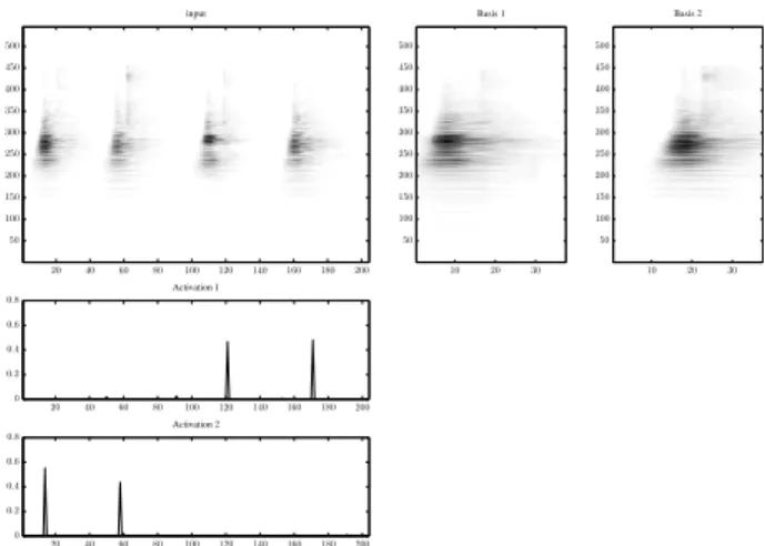
• Expectation step: P(z, τ |ω, t) = P P(z)P (ω, τ |z)P (t − τ |z) z P τP(z)P (ω, τ |z)P (t − τ |z) (2) Activation 2 Activation 1 Basis 2 Basis 1 input 20 40 60 80 100 120 140 160 180 200 20 40 60 80 100 120 140 160 180 200 10 20 30 10 20 30 20 40 60 80 100 120 140 160 180 200 0 0.2 0.4 0.6 0.8 0 0.2 0.4 0.6 0.8 50 100 150 200 250 300 350 400 450 500 50 100 150 200 250 300 350 400 450 500 50 100 150 200 250 300 350 400 450 500

Figure 1: SIPLCA applied to a sequence of footsteps (z = 2).

Top left: input CQT spectrogram, right: extracted basis matrices, bottom: extracted component activations.

Equation (2) is computed through the model of (1) using Bayes’ theorem and expresses the posterior of the unknown variables over the known data. The unknown matrices are initialized with random values. The update rules of (2)-(5) are iterated until convergence. An example of the SIPLCA algorithm is given in Fig. 1, where SIPLCA is applied to a recording of footsteps with z = 2. The

activations P(t|z) of the footsteps are clearly seen as spikes.

In [13], sparsity constraints are applied to the model in or-der to provide as meaningful solutions as possible. The sparsity constraints are applied using an entropic prior, by modifying the update equations in the maximization step. In the present work, we will encourage sparsity on the component activation P(t|z) in

order to derive informative basis matrices.

3. PROPOSED METHOD 3.1. Motivation

The motivation behind the model proposed in this paper is to in-clude another level of temporality, which controls the appearance of the time-frequency patches in a recording. These temporal con-straints can be supported by incorporating HMMs within the SIPLCA model. Ideally, the component activation function would con-sist of zeros in case of inactivity and ones at the time instants where an event would appear. Each HMM can represent a cer-tain component, which would be represented using a two-state, on/off model. This on/off model would serve as an event indicator function, which would enforce temporal constraints in the audi-tory scene activation matrix. Thus, in this case we propose a novel

(4)

model which supports time-frequency patches for auditory scene characterization and also controls the temporal succession of these scenes.

This work will extend the temporally-constrained convolutive probabilistic model for pitch detection presented in [14], which utilised shift-invariance over log-frequency for spectra instead of performing shift-invariance over time for time-frequency basis as in this work. These models which combine spectral factorization techniques with HMMs were first introduced in [15], where the non-negative HMM algorithm was proposed.

3.2. HMM-constrained Shift-invariant PLCA

This proposed temporally-constrained model takes as input a nor-malized spectrogram Vω,tand decomposes it as a series of

time-frequency patches. Also produced is a component activation ma-trix, as well as component priors. The activation of a each acoustic component is controlled via a 2-state HMM. The model can be formulated as: Vω,t≈ P (ω, t) = X z P(z)X q(z)t P(ω, τ |z) ∗τP(t|z)P (q(z)t |t) (6) where qt(z) is the state sequence for the z-th component, z =

1, . . . , Z. SinceP

q(z)t

P(qt(z)|t) = 1, we can revert to the

non-temporally constrained model of the previous section. Thus in the model, the desired source activation is given by P(z|t)P (qt(z) =

1|t).

The activation sequence for each component is constrained us-ing a correspondus-ing HMM, which is based on the produced source activation P(z, t) = P (z)P (t|z). In terms of the activations, the

component-wise HMMs can be expressed as:

P(¯z) =X ¯ q(z) P(q₁(z))Y t P(q(z)_t+1|q(z)t ) Y t Pt(zt|qt(z)) (7)

wherez refers to the sequence of activations for a given compo-¯

nent z, P(q1(z)) is the prior probability, P (q (z) t+1|q

(z)

t ) is the

tran-sition matrix for the z-th component, and Pt(zt|q(z)t ) is the

ob-servation probability (zt refers to the activation at frame t). The

observation probability for an active component is defined using a sigmoid curve:

Pt(zt|qt(z)= 1) =

1

1 + e−P(z,t)−λ (8)

where λ is a parameter that controls the component activation (a high value will lead to a low observation probability, leading to an ‘off’ state). The formulation of the observation function is similar to the one used for multiple note tracking in [16].

As in the model of Section 2, the unknown parameters in the model can be estimated using the EM algorithm [12]. For the

Ex-pectation step, we compute the posterior for all the hidden

vari-ables: P(z, τ, q(1)t , . . . , q (Z) t |¯z, ω, t) = P(q(1)t , . . . , q (Z) t |¯z)P (z, τ |q (1) t , . . . , q (Z) t , ω, t) (9)

Since we are utilising independent HMMs, the joint probability for all hidden source states is given by:

Pt(q(1)t , . . . , q (Z) t |¯z) = Z Y z=1 Pt(q(z)t |¯z) (10) where Pt(q(z)t |¯z) = Pt(¯z, qt(z)) P q(z)t Pt(¯z, q(z)t ) = αt(q (z) t )βt(qt(z)) P q(z)t αt(q(z)t )βt(q(z)t ) (11) and αt(q(z)t ), βt(q(z)t ) are the forward and backward variables for

the z-th HMM [17], which can be computed recursively:

P(z) = P ω,τ,t P qt(z) Vω,tP(z, τ, qt(1), . . . , q (Z) t |ω, t) P z,ω,τ,t P q(z)t Vω,tP(z, τ, q(1)t , . . . , q (Z) t |ω, t) (16) P(ω, τ |z) = P t P q(z)t Vω,tP(z, τ, q(1)t , . . . , q (Z) t |ω, t) P ω,τ,t P q(z)t Vω,tP(z, τ, q(1)t , . . . , q (Z) t |ω, t) (17) P(t|z) = P ω,τ P q(z)t Vω,t+τP(z, τ, qt(1), . . . , q (Z) t |ω, t + τ ) P t,ω,τ P q(z)t Vω,t+τP(z, τ, q(1)t , . . . , q (Z) t |ω, t + τ ) (18) P(q(z)_t+1|qt(z)) = P tP(q (z) t , q (z) t+1|¯z) P q_t+1(z) P tP(q (z) t , q (z) t+1|¯z) (19) P(q₁(z)) = P1(q1(z)|¯z) (20) whereP q(z)t =P q(1)t · · ·P qt(Z)

. Eq. (20) updates the compo-nent prior using the posterior of eq. (11). Thus, the update equa-tions of the proposed model are a combination of the SIPLCA update rules and the forward-backward HMM algorithm. The fi-nal event activation is given by the activation for each component given by the model and the probability for an active state for the corresponding component:

P(z, t, qt(z)= 1) = P (z)P (t|z)P (q

(z)

(5)

CQT PROPOSED MODEL CONVERSION TO CEPSTRUM COEFS AUDIO _DISTANCE COMPUTATION Wl cl Vω,t cm D(l, m)

Figure 2: Diagram for the proposed acoustic scene classification system.

5 4

3 2

1

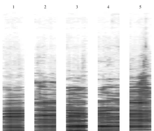
Figure 3: Extracted time-frequency basis matrices using the

pro-posed model.

As in the SIPLCA model of Section 2, sparsity constraints are applied to P(t|z) using the entropic prior of [13] in order to obtain

a sparse component activation. In Fig. 3, extracted time-frequency basis matrices can be seen, from a recording employed for eval-uation (described in Section 4) using the proposed method with

z = 5. Components corresponding to different acoustic events

can be seen in the figure. For all the experiments performed in this paper, the length of each basis has been set to 400ms.

3.3. Acoustic Scene Distance

For computing the distance between acoustic scenes, we first com-pute the constant-Q transform [18] of each 44.1 kHz recording with a log-frequency resolution of 5 bins per octave and an 8-octave span with 27.5 Hz set as the lowest frequency. The step size is set to 40 ms. Afterwards, time-frequency basis matrices are extracted using the proposed HMM-constrained SIPLCA algo-rithm of Section 3.2 with R= {10, 25, 50} bases and λ = 0.005

(the value was set after experimentation). Sparsity was enforced

to P(t|z) using an entropic prior method of [13] with sparsity

pa-rameter values sH= {0, 0.1, 0.2, 0.5}. In all cases the length of

each basis is set to 400 ms.

For each basis W = P (ω, τ |z), very small values are replaced

by the median value of W . Afterwards, a vector of 13 cepstral coefficients is computed for each basis frame, in order to result in a compact representation for computational speed purposes. In order to convert a vector w[k](k = 1, . . . , K) into cepstral coefficients,

we employ the formula presented in [19]:

ci= K X k=1 log(w[k]) cos „ i „ k−1 2 « π K « (22) where i= 1, . . . , 13. Each vector of cepstral coefficients is then

normalized to the range [0,1] region. Thus, the first coefficient that corresponds to the DC component of the signal is dropped. Finally, for each time-frequency basis, the coefficients are summed together over time, thus resulting in a single vector representing a basis.

For computing the distance between a scene l and a scene m, we employ the same steps as in [4]. Firstly, we compute the ele-ment wise distance between a basis Wl(r), r = 1, . . . , R and the

nearest basis of dictionary Wm:

dr(l, m) = min

j∈[1,R]||Wl(r) − Wm(j)|| (23)

The final distance between two acoustic scenes is defined as:

D(l, m) =

R

X

r=1

dr(l, m) + dr(m, l) (24)

Equation (24) is formulated in order for the distance measure be-tween two scenes to be symmetric. In the end, the acoustic scene distance matrix D is used for evaluation.

We acknowledge that quantifying the distance between two basis vectors by considering the Euclidean distance of their time average most probably leads to a loss of descriptive power of our model. This choice is made for tractability purposes. Indeed, for the corpus used in this study and 50 bases per item, building the matrix D involves comparing about106_{bases. Finding an efficient}

way of considering the time axis during the distance computation is left for future research.

4. EVALUATION 4.1. Dataset

For the acoustic scene classification experiments we employed the dataset created by J. Tardieu [5]. The dataset was originally cre-ated for a perceptual study on free- and forced-choice recogni-tion of acoustic scenes by humans. It contains 66 44.1 kHz files recorded in 6 different train stations (Avignon, Bordeaux, Lille Flandres, Nantes, Paris Est, Rennes). Each file is classified into a ‘space’, which corresponds to the location this file was recorded: platforms, halls, corridors, waiting room, ticket offices, shops. The recordings contain numerous overlapping acoustic events, making even human scene classification a nontrivial task. In Table 1, the class distribution for the employed dataset can be seen. In addition to the ground truth included for each recording, an additional scene label is included as a result of the forced-categorisation perceptual study performed in [5].

(6)

Scene Platform Hall Corridor Waiting Ticket Office Shop

No. Samples 10 16 12 13 10 5

Table 1: Class distribution in the employed dataset of acoustic

scenes.

4.2. Evaluation metrics

For evaluation, we employed the same set of metrics that were used in [4] for the same experiment, namely the mean average pre-cision (MAP), the 5-prepre-cision, and the classification accuracy of a nearest neighbour classifier. The MAP and 5-precision metrics are utilised for ranked retrieval results, where in this case the ranking is given by the values of the distance matrix D. MAP is able to provide a single-figure metric across recall levels and can describe the global behaviour of the system. It is computed using the av-erage precision, which is the avav-erage of the precision obtained for the set of top n documents existing after each relevant document is retrieved. The 5-precision is the precision at rank 5 (which cor-responds to the number of samples in the smallest class), which describes the system performance at a local scale.

Regarding the classification accuracy metric, for each row of

D we apply the k-nearest neighbour classifier with 11 neighbours,

which corresponds to the average number of samples per class.

4.3. Results

Acoustic scene classification experiments were performed using the SIPLCA algorithm of [7] and the proposed SIPLCA algorithm with temporal constraints (TCSIPLCA). Comparative results are also reported using a bag-of-frames (BOF) approach of [6] re-ported in [4]. The BOF method computes several audio features which are fed to a Gaussian mixture model (GMM) classifier. The NMF method of [4] was also implemented and tested. Results are also compared with the human perception experiment reported in [5]. Experiments were performed using different dictionary sizes

R and sparsity parameters sH (details on the range of values can

be seen in Section 3.3).

The best results using each employed classifier are presented in Table 2. It can be seen that the proposed temporally-constrained SIPLCA model outperforms all other classifiers using both met-rics, apart from the human forced categorisation experiment. The proposed method slightly outperforms the standard SIPLCA algo-rithm, which in turn outperforms the NMF algorithm. It can also be seen that the BOF method is clearly not suitable for such ex-periment, since the audio features employed in this method are more appropriate for non-overlapping events, whereas the dataset that is utilised contains concurrent events. However, it can be seen that the human categorisation experiment from [5] outperforms all other approaches.

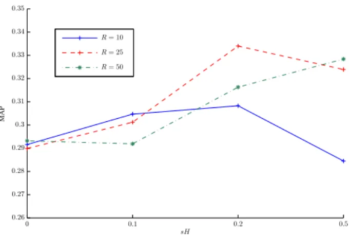
More detailed results for the SIPLCA algorithm using differ-ent sparsity parameter values and a differdiffer-ent number of extracted bases (R) can be seen in Fig. 4. It can be seen that in all cases, enforcing sparsity improves performance. It can also be seen that the best performance is reported for R = 25, although the

per-formance of the system using R = 50 improves when greater

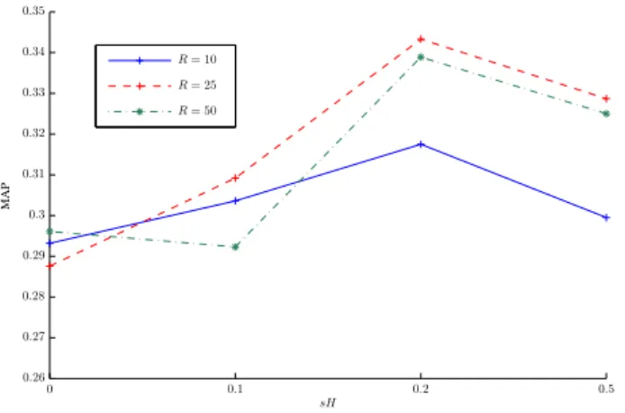
sparsity on P(t|z) is encouraged. Detailed results for the

pro-posed TCSIPLCA method can be seen in Fig. 5, using different dictionary sizes and sparsity values. It can be seen that the perfor-mance reaches a peak when sH = 0.2, for the case of R = 25.

Classifier MAP 5-Precision Human Perception [5] 0.62 0.73 Random 0.25 0.18 BOF [6] 0.24 0.18 NMF (R= 50, sH = 0.99) 0.32 0.29 SIPLCA (R= 25, sH = 0.2) 0.33 0.35 TCSIPLCA (R= 25, sH = 0.2) 0.34 0.36

Table 2: Best MAP and 5-precision results for each model.

R= 50 R= 25 R= 10 sH M A P 0 0.1 0.2 0.5 0.26 0.27 0.28 0.29 0.3 0.31 0.32 0.33 0.34 0.35

Figure 4: Acoustic scene classification results (MAP) using the

SIPLCA algorithm with different sparsity parameters and dictio-nary size (R).

When using a dictionary size of R= 50, the performance of the

proposed method is slightly decreased. Thus, selecting the appro-priate number of components is important in the performance of the proposed method, since using too many components will lead to a parts-based representation which in the unsupervised case will lead to non representative dictionaries. Likewise, selecting too few bases will lead to a less descriptive model of the input signal.

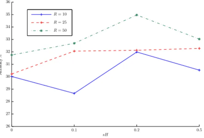
Regarding classification accuracy using 11-nearest neighbours, results are shown in Table 3. Again, the TCSIPLCA method out-performs all the other automatic approaches. In this case however, the NMF approach from [4] outperforms the SIPLCA algorithm by 0.5%. For the TCSIPLCA algorithm, the best performance is again reported for sH= 0.2, while for the NMF approach the best

performance is reported for sH= 0. It should also be noted that

regarding dictionary size, the best results are reported for R= 50.

Detailed classification results using the SIPLCA and TCSIPLCA methods can be seen in Figures 6 and 7, respectively.

It should also be noted that some experiments were performed by selecting only basis vectors that correspond to a sparse activa-tion P(t|z). In the PLCA domain, the sparseness criterion can be

given by maximizing the l2 norm as in [20], due to the fact that

all elements of the activation matrix take values between 0 and 1. However, the performance of the SIPLCA and TCSIPLCA al-gorithms in fact decreased slightly when selecting only the basis vectors that corresponded to the sparsest activations. This issue may be addressed in the future by enforcing sparsity only to cer-tain components that represent salient events and keeping the rest of the components (which could represent noise) without

(7)

enforc-R= 50 R= 25 R= 10 sH M A P 0 0.1 0.2 0.5 0.26 0.27 0.28 0.29 0.3 0.31 0.32 0.33 0.34 0.35

Figure 5: Acoustic scene classification results (MAP) using the

TCSIPLCA algorithm with different sparsity parameters and dic-tionary size (R).

ing sparsity.

5. CONCLUSIONS

In this work we proposed a method for modeling and classifying acoustic scenes using shift-invariant probabilistic methods. The shift-invariant probabilistic latent component analysis algorithm was utilised for learning time-frequency basis matrices from an in-put acoustic signal in an unsupervised manner. An algorithm was proposed for incorporating temporal constraints to the SIPLCA model using hidden Markov models, in order to constrain the acti-vation of each event in the signal. In the classification stage, each extracted time-frequency basis is converted into a compact vec-tor of cepstral coefficients for computational speed purposes. The employed dataset consisted of recordings taken from six types of scenes at different train stations. Comparative experiments were performed using a standard non-negative matrix factorization ap-proach, as well as a bag-of-frames algorithm which is based on computing audio features. Results show that using shift-invariant models for learning time-frequency basis matrices improves clas-sification performance. Moreover, incorporating temporal straints in the SIPLCA model as well as enforcing sparsity con-straints in the component activation resulted in improved classifi-cation performance.

However, the classification performance of the proposed com-putational methods is still significantly lower than the human forced categorisation task presented in [5]. We acknowledge that this performance is in our case an upper bound that may not even be reached by purely data-driven methods since humans most proba-bly make extensive use of prior knowledge but the significant gap between the human and computational performances indicates that there is potentially room for improvement on the computational side.

In order to improve spectrogram factorization techniques such as NMF and SIPLCA, additional constraints and knowledge need to be incorporated into the models. A hierarchical model which would consist of event classes and component subclasses would result in a richer model, but would also require prior information on the shape of each event in order to result in meaningful basis matrices. Prior information can be provided by utilising training

Classifier Accuracy % Human Perception [5] 54.8% Random 16.6% BOF [6] 19.7% NMF (R= 50, sH = 0) 34.1% SIPLCA (R= 25, sH = 0.5) 33.6% TCSIPLCA (R= 50, sH = 0.2) 35.0%

Table 3: Best classification accuracy for each model.

R= 50 R= 25 R= 10 sH A cc u ra cy % 0 0.1 0.2 0.5 25 26 27 28 29 30 31 32 33 34 35

Figure 6: Classification accuracy (%) using the SIPLCA algorithm

with different sparsity parameters and dictionary size (R).

samples of non-overlapping acoustic events. Also, an additional sparseness constraint could be imposed in the activation matrix, in order to control the number of overlapping components present in the signal (instead of enforcing sparsity as in the present work). In addition, instead of using a first-order Markov model for imposing temporal constraints, a more complex algorithm which would be able to model the duration of each event, such as a semi-Markov model [21] can be employed. Finally, finding an efficient way of comparing extracted time frequency patches is also important. In this respect, we believe that lower bounding approaches to the dy-namic time warping (DTW) technique are of interest [22].

6. REFERENCES

[1] D. L. Wang and G. J. Brown (Eds.), Computational

audi-tory scene analysis: Principles, algorithms and applications,

IEEE Press/Wiley-Interscience, 2006.

[2] A. Mesaros, T. Heittola, and A. Klapuri, “Latent semantic analysis in sound event detection,” in European Signal

Pro-cessing Conference, Barcelona, Spain, Aug. 2011.

[3] C. Cotton and D. Ellis, “Spectral Vs. spectro-temporal fea-tures for acoustic event detection,” in IEEE Workshop on

Applications of Signal Processing to Audio and Acoustics,

New Paltz, USA, Oct. 2011, pp. 69–72.

[4] Benjamin Cauchi, “Non-negative matrix factorisation ap-plied to auditory scenes classification,” M.S. thesis, ATIAM (UPMC / IRCAM / TELECOM ParisTech), Aug. 2011.

(8)

R= 50 R= 25 R= 10 sH A cc u ra cy % 0 0.1 0.2 0.5 26 27 28 29 30 31 32 33 34 35 36

Figure 7: Classification accuracy (%) using the TCSIPLCA

algo-rithm with different sparsity parameters and dictionary size (R).

[5] J. Tardieu, P. Susini, F. Poisson, P. Lazareff, and S. McAdams, “Perceptual study of soundscapes in train sta-tions,” Applied Acoustics, vol. 69, no. 12, pp. 1224–1239, 2008.

[6] J.J. Aucouturier, B. Defreville, and F. Pachet, “The bag-of-frames approach to audio pattern recognition: a sufficient model for urban soundscapes but not for polyphonic music,”

Journal of the Acoustical Society of America, vol. 122, no. 2,

pp. 881–891, 2007.

[7] P. Smaragdis and B. Raj, “Shift-invariant probabilistic la-tent component analysis,” Tech. Rep., Mitsubishi Electric Research Laboratories, Dec. 2007, TR2007-009.

[8] P. Smaragdis, B. Raj, and Ma. Shashanka, “A probabilistic latent variable model for acoustic modeling,” in Neural

In-formation Processing Systems Workshop, Whistler, Canada,

Dec. 2006.

[9] P.D. O’Grady and B.A. Pearlmutter, “Convolutive non-negative matrix factorisation with a sparseness constraint,” in

2006 16th IEEE Signal Processing Society Workshop on Ma-chine Learning for Signal Processing, Sept. 2006, pp. 427–

432.

[10] G. Mysore and P. Smaragdis, “Relative pitch estimation of multiple instruments,” in IEEE International Conference on

Acoustics, Speech, and Signal Processing, Taipei, Taiwan,

Apr. 2009, pp. 313–316.

[11] E. Benetos and S. Dixon, “Multiple-instrument polyphonic music transcription using a convolutive probabilistic model,” in 8th Sound and Music Computing Conference, Padova, Italy, July 2011, pp. 19–24.

[12] A. P. Dempster, N. M. Laird, and D. B. Rubin, “Maxi-mum likelihood from incomplete data via the EM algorithm,”

Journal of the Royal Statistical Society, vol. 39, no. 1, pp. 1–

38, 1977.

[13] P. Smaragdis, “Relative-pitch tracking of multiple arbitary sounds,” Journal of the Acoustical Society of America, vol. 125, no. 5, pp. 3406–3413, May 2009.

[14] E. Benetos and S. Dixon, “A temporally-constrained con-volutive probabilistic model for pitch detection,” in IEEE

Workshop on Applications of Signal Processing to Audio and Acoustics, New Paltz, USA, Oct. 2011, pp. 133–136.

[15] G. Mysore, A non-negative framework for joint modeling of

spectral structure and temporal dynamics in sound mixtures,

Ph.D. thesis, Standford University, USA, June 2010. [16] G. Poliner and D. Ellis, “A discriminative model for

poly-phonic piano transcription,” EURASIP Journal on Advances

in Signal Processing, , no. 8, pp. 154–162, Jan. 2007.

[17] L. R. Rabiner, “A tutorial on hidden Markov models and selected applications in speech recognition,” Proceedings of

the IEEE, vol. 77, no. 2, pp. 257–286, Feb. 1989.

[18] C. Schörkhuber and A. Klapuri, “Constant-Q transform tool-box for music processing,” in 7th Sound and Music

Comput-ing Conference, Barcelona, Spain, July 2010.

[19] J. C. Brown, “Computer identification of musical instru-ments using pattern recognition with cepstral coefficients as features,” Journal of the Acoustical Society of America, vol. 105, no. 3, pp. 1933–1941, Mar. 1999.

[20] P. Smaragdis, “Polyphonic pitch tracking by example,” in

IEEE Workshop on Applications of Signal Processing to Au-dio and Acoustics, New Paltz, USA, Oct. 2011, pp. 125–128.

[21] S. Z. Yu, “Hidden semi-Markov models,” Artificial

Intelli-gence, vol. 174, no. 2, pp. 215 – 243, 2010.

[22] Y. Zhang and J. Glass, “An inner-product lower-bound es-timate for dynamic time warping,” in IEEE International

Conference on Audio, Speech and Signal Processing, Prague,