HAL Id: hal-03023318
https://hal.archives-ouvertes.fr/hal-03023318v1
Preprint submitted on 25 Nov 2020 (v1), last revised 26 Nov 2020 (v2)
HAL is a multi-disciplinary open access
archive for the deposit and dissemination of
sci-entific research documents, whether they are
pub-lished or not. The documents may come from
teaching and research institutions in France or
abroad, or from public or private research centers.
L’archive ouverte pluridisciplinaire HAL, est
destinée au dépôt et à la diffusion de documents
scientifiques de niveau recherche, publiés ou non,
émanant des établissements d’enseignement et de
recherche français ou étrangers, des laboratoires
publics ou privés.
Modeling and finite element simulation of multi-sphere
swimmers
Luca Berti, Vincent Chabannes, Laetitia Giraldi, Christophe Prud’Homme
To cite this version:
Luca Berti, Vincent Chabannes, Laetitia Giraldi, Christophe Prud’Homme. Modeling and finite
ele-ment simulation of multi-sphere swimmers. 2020. �hal-03023318v1�
MULTI-SPHERE SWIMMERS
Luca Berti
Cemosis, IRMA UMR 7501, CNRS Universit´e de Strasbourg, France
Vincent Chabannes Cemosis, IRMA UMR 7501, CNRS
Universit´e de Strasbourg, France [email protected]
Laetitia Giraldi
CALISTO team, INRIA, Universit´e Cˆote d’Azur CEMEF, France
Christophe Prud’homme Cemosis, IRMA UMR 7501, CNRS
Universit´e de Strasbourg, France [email protected]
A
BSTRACTWe propose a numerical method for the finite element simulation of micro-swimmers composed of several rigid bodies moving relatively to each other. Three distinct formulations are proposed to impose the relative velocities between the rigid bodies. We validate our model on the three-sphere swimmer, for which analytical results are available.
Keywords Stokes in moving domains with articulated rigid bodies, 3-Sphere swimmer, Finite Element Method and ALE Formulation
Version franc¸aise abr´eg´ee
Dans cet article nous proposons une m´ethode num´erique pour la simulation aux ´el´ements finis d’une classe de micro-nageurs. Ces nageurs sont compos´es par diff´erents corps rigides qui peuvent bouger les uns par rapport aux autres. Nous appliquons notre m´ethode sur un exemple de micro-nageur connu sous le nom de Three-sphere swimmer.
1
Introduction
The dynamics of immersed rigid and deformable bodies in low Reynolds number flows has been extensively studied for its applications to suspension phenomena and the motion of biological micro-organisms [6, 5].
Different numerical methods are used to study these dynamics, such as the Boundary Element method, which dis-cretizes the boundary integral form of Stokes equations [12]; Resistive Force Theory, where the hydrodynamical inter-actions are approximated by suitable coefficients [1]; the Finite Element method, where the fluid domain is discretized and fitted [8] or unfitted [4] meshes are used for the immersed bodies. In the following, the focus will be on the Finite Element method with body-fitted mesh, where the Arbitrary Lagrangian-Eulerian formalism is used to to solve the motion of the fluid domain. While this choice was dictated by its straightforward extension to non-Newtonian fluids and interactions with immersed elastic bodies, the present article is concerned with the simulation of swimmers com-posed of multiple rigid bodies that move relatively to each other. The main examples are micro-swimmers comcom-posed of spherical bodies, which have been extensively studied via the fundamental solution associated to an immersed rigid sphere [9, 7, 2]. Theoretical and numerical results make these swimmers ideal benchmarking models.
In this paper we propose a numerical method, based on finite elements and the Arbitrary-Lagrangian Eulerian formula-tion, that allows the simulation of micro-swimmers composed of rigid parts moving relatively to each other, extending [8] to self-propelled swimmers. We illustrate our method by recovering the motion of the three-sphere swimmer, as reported in [9].
Modeling and finite element simulation of multi-sphere swimmers
2
Mathematical formulation of the problem
In this section we recall the formulation of a generic swimming problem in Stokes flow. Let F0 ⊆ Rd, d = 3, be the
initial configuration of the fluid domain and At: F0→ Ftthe smooth function that maps the reference fluid domain
onto the domain Ftoccupied by the fluid at time t. Let S0 ⊆ Rdbe the domain occupied by the swimmer at time
t = 0 and St ⊆ Rd be the domain it occupies at time t. Let (u, p) be the fluid velocity and pressure defined over
Ft, µ the viscosity, f the fluid volume forces. We denote by U and ω the translational and angular velocities of the
swimmer, by xCM its center of mass and by m and J its volume and geometric inertia tensor. The coupled problem, expressing the kinematic and dynamic coupling of the fluid with the swimmer, reads
−µ∆u + ∇p = f, in Ft, ∇ · u = 0, in Ft, u = U + ω × (x − xCM(t)) + ud(t) ◦ A−1t , on ∂St, m ˙U = −Ff luid, J ˙ω = −Mf luid. (1)
where Ff luid and Mf luid denote the global fluid forces and torques acting on the boundary of the swimmer. The
function ud(t) denotes the time derivative of body deformation, and it is the driving mechanism of the whole motion,
making the otherwise stationary problem time-dependent.
The map At(x) is defined as At(x) = x + φt(x), where φt(x) is the solution of the following Laplace problem
(∆φt(x) = 0 in F0,
˙
φt(x) = U + ω × (x − xCM(t)) + ud(t), on ∂S0.
(2)
3
The articulated micro-swimmer
The articulated micro-swimmer is composed of n rigid bodies among which a reference body Bn is identified. This
body is linked to all the other bodies Bi, for i ∈ {1 . . . n − 1}, by thin and hydrodynamically negligible arms. The
length of these links can be changed via “internal motors” that impose a relative speed between the bodies, leading to self-propulsion.
In principle, each Bican have a different shape, but we choose to work with spheres for benchmarking purposes. In
fact, the motion of some multi-sphere swimmers can be analytically computed by using the appropriate Green kernel of Stokes equations [9].
In this section the motion of n independent bodies is first described, by recalling the formulation in [8]. After that, we present the modified formulation that takes into account the relative velocities between the bodies. In the end, we propose few equivalent methods that allow the imposition of the velocity constraints.
3.1 Motion of n independent bodies
Using the same notations as before, the problem of n independent bodies moving in a Stokes fluid reads −µ∆u + ∇p = f, in Ft, ∇ · u = 0, in Ft, u = Ui+ ωi× (x − xCMi (t)), i = 1 . . . n, on ∂Bi, miU˙i= −Ff luid, i = 1 . . . n, Jiω˙i= −Mf luid, i = 1 . . . n. (3)
In this case ud(t) = 0, as the bodies move independently of each other and no deformation is present. Hence,
At(x) = x + φt(x), where φt(x) is the solution of the Laplace problem
(∆φt(x) = 0 in F0,
˙
φt(x) = Ui+ ωi× (x − xCMi (t)), on ∂Bi.
(4)
In this formulation, the body motion is dictated by fluid stresses only. We now address the variational formulation of (3) and look for a solution (u, p, Ui, ωi) ∈ [H1(Ft)]d× L2(Ft) × [Rd]n× [Rd]nto the weak formulation of the
problem.
Let (˜u, ˜p, ˜Ui, ˜ωi) ∈ [H1(Ft)]d× L2(Ft) × [Rd]n× [Rd]ndenote the test functions. The variational formulation reads 2µ Z Ft D(u) : D(˜u) dx − n X i=1 Z ∂Bi (−pI + 2µD(u))~n · ˜u dS − Z Ft p∇ · ˜u dx = Z Ft f · ˜u dx, (5) Z Ft ˜ p∇ · u dx = 0, (6) m ˙Ui· ˜Ui= − Z ∂Bi (−pI + 2µD(u))~n · ˜UidS, i = 1 . . . n, (7) J ˙ωi· ˜ωi= − Z ∂Bi (−pI + 2µD(u))~n × (x − xCMi ) · ˜ωidS, i = 1 . . . n, (8)
where D(u) = 12(∇u + ∇uT).
Following [8], we choose (˜u, ˜Ui, ˜ωi) ∈ [H1(F )]d× [Rd]n× [Rd]nsatisfying u = Ui+ ωi× (x − xCMi ) on ∂Bi.
These test functions form a subspace of [H1(F
t)]d× [Rd]n× [Rd]n, and they satisfy the relationship
Z ∂Bi (−pI + 2µD(u))~n · ˜u dS = Z ∂Bi (−pI + 2µD(u))~n · ˜UidS + Z ∂Bi (−pI + 2µD(u))~n × (x − xCMi ) · ˜ωidS, (9)
that combines the boundary terms in equations (5)-(7)-(8). The “compact” reformulation 2µ Z Ft D(u) : D(˜u) dx − Z Ft p∇ · ˜u dx + n X i=1 miUi· ˜Ui+ Jiωi· ˜ωi = Z Ft f · ˜u dx. (10) of equations (5)-(7)-(8) shows that boundary terms have been absorbed by the choice of the finite element spaces. 3.2 The constraints on relative velocities
Among the n bodies composing the articulated swimmer, we identify Bnas the reference body. The velocities Uiof
all the other bodies Bi, i = 1 . . . n − 1, are expressed as functions of Unvia constraints of the form
Ui = Un+ Win(t), i = 1 . . . n − 1, (11)
where Win(t) represents the relative velocity between Biand Bn. The addition of these constraints to (3) completes
the formulation of the swimming problem for the articulated swimmers. We notice that the resulting system is a particular instance of the general case presented in (1), where ud(t) is given by combining the constraints in (11).
The formulation we just described applies directly to the three-sphere swimmer [9], an articulated swimmer composed of three aligned spheres. Here the reference body Bn = B3is the central sphere, which is connected by extensible
arms to the other two spheres B1and B2. The formulation can be applied as well to the planar three-sphere swimmer
[7] or to the four-sphere swimmer [2], whose spherical bodies are placed on the vertices of an equilateral triangle or tetrahedron, respectively. In those cases, the relative velocity vectors Winshould be carefully computed, as each
extensible arm connects Bito the barycenter of the swimmer, and not to Bndirectly as in the case of the three-sphere
swimmer.
3.3 Discrete and algebraic formulation
Let us consider a geometrical discretization Fh of the fluid domain using simplices. The fluid problem is then
discretized using an inf-sup stable pair of conforming finite element spaces Xh(Fh) × Bh(Fh) for (uh, Bh) and
(Uj, ωj) ∈ [Rd]n× [Rd]n.
Since the fluid velocity satisfies u = Ui+ ωi× (x − xCMi ) on ∂Bi, the degrees of freedom u∂Bi that lie on ∂Bi
are treated differently from the remaining ones, that we denote by uI. Indeed, u∂Bi are expressed as a function of
(Ui, ωi).
At first, equations (5)-(8) are discretized by ignoring the constraint u = Ui+ ωi× (x − xCMi ) on ∂Bi. Then, via the
operator P = I 0 0 0 0 0 P˜Ui P˜ωi 0 0 0 I 0 0 0 0 0 I 0 0 0 0 0 I 0 0 0 0 0 I , (12)
Modeling and finite element simulation of multi-sphere swimmers
that satifies the equation
(uI, u∂Bi, Ui, ωi, p)
T = P(u
I, Ui, ωi, p)T,
the change of finite element basis, from the standard formulation to the constrained one, is performed. In (12), ˜PUi
and ˜Pωiare the interpolation operators that allow the expression of u∂Bi as a function of Uiand ωi.
The constraints on the relative velocities between the bodies can be imposed via Lagrange multipliers, through a modification of the operator P or by modifying the matrix that results from the discretization of the fluid problem. The first method is the least invasive: additional equations and unknowns are added to a pre-existing discretized problem of n independent bodies in a Stokes fluid, as described in (3). Lagrange multipliers αi ∈ Rd, i = 1 . . . n − 1
are introduced to impose the constraints on the translational velocities Ui onto the differential formulation. The
previous constraint will appear in the equations that describe the rigid body motion of the solid bodies: equations (7) will be substituted by m ˙Ui· ˜Ui+ αi· ˜Ui= − Z ∂Bi (−pI + 2µD(u))~n · ˜UidS, i = 1 . . . n − 1, (13) m ˙Un· ˜Un− n−1 X i=1 αi· ˜Un= − Z ∂Bn (−pI + 2µD(u))~n · ˜UndS, (14) αi· (Ui− Un) = αi· Win, i = 1 . . . n − 1. (15)
The addition of Lagrange multipliers entails the modification of P by providing an additional identity matrix of size d(n − 1) × d(n − 1) on the diagonal.
Instead of using Lagrange multipliers to constrain the translational velocities, a modification of the operator P could give the same results. In terms of finite element spaces, this consists in reducing the constrained finite element space to basis functions that satisfy u = Un+ ωn× (x − xCMn (t)) + ud(t), with ud(t) function of Win.
The dn × dn block that corresponds to the translational speeds, that presently is an identity matrix Idn, would be
substituted by a block of the form
B1{ Bi{ Bn{ "I d . . . 0d . . . −Id 0d . . . Id . . . −Id −Id . . . −Id . . . Id # . (16)
This modification must be applied directly to the construction of P, because an a posteriori change of the operator would be too costly in terms of operations on the compactly stored matrix. The relative velocities will then be imposed on the right-hand side of the problem, as the known part of the body velocity.
The last modification is even more invasive, and it consists in modifying the system matrix and right-hand side by substituting (7) with (miUi− mnUn) · ˜Ui= Win(t) · ˜Ui, i = 1 . . . n − 1, mnU˙n· ˜Un= − Z ∂Bn (−pI + 2µD(u))~n · ˜UndS. (17)
4
The three-sphere micro-swimmer
The three-sphere micro-swimmer [9] is a three-dimensional swimmer composed of three aligned spheres having the same radius R. The two outer spheres are connected to the central one by extensible links, and the propulsion of the swimmer is ensured by changing the lengths of the connecting arms between two fixed values. The arm shrinkage is performed in a non-reversible fashion, in order to break the time-reversal symmetry of the Stokes equations, with a constant relative speed between the central sphere and the approaching one. For example, if the left arm is shrinking and the right arm keeps its length fixed, the translational speed U3 and U2of the central and right sphere coincide,
while the speed of the left sphere, moving with relative speed W13with respect to the center sphere, will be U3+ W13.
The (non-reciprocal) stroke is composed of 4 steps, as shown in Figure 1, where the lengths of the two arms are alternatively modified.
A quantitative example of swimming is presented in [9]: if D = 10R is the length of each link in its rest position and ε = 4R is the maximal variation for the length of each arm (leaving a link length of 6R when the arms are completely shrunk), the center sphere is displaced by 0.16R in the positive direction at the end of the 4-step stroke. In the first
L L B1 B3 B2 L-a L L-a L-a L L-a L L
Figure 1: Representation of the three-sphere swimmer and its swimming gait. The gait is composed of four strokes in which one of the arms is alternatively shrunk or elongated. The alternation guarantees the non-reciprocity of the motion.
CM_evolution_1.png
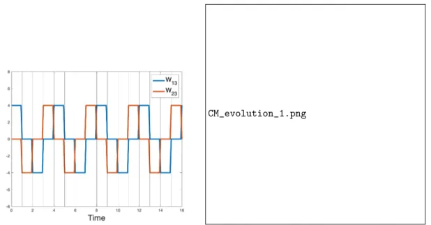
Figure 2: The left figure presents the relative speed W13, between the central and left sphere, and the relative speed
W23, between the central and right sphere, as functions of time. The right figure shows, in blue, the position of the
central sphere during the 4-step stroke. The red line intersects the trajectory of the central sphere at the red circles, which mark the 0.08R and 0.16R displacements predicted in [9] after 2 and 4 steps composing the swimming stroke.
step, the travelled distance is 1.35R in the negative direction; in the second step, it is 1.44R in the positive direction; in the third step, it is 1.44R in the positive direction; in the fourth step, it is 1.35R in the negative direction.
Using the aforementioned Lagrange multipliers formulation, we are able to recover the displacement at each step of the 4-step stroke reported in [9]. Figure 2, on the left, translates the steps of the body deformation in terms of relative velocities between the central and lateral spheres. Figure 2, on the right, represents the motion of B3during several
repetitions of the 4-step stroke. The results were obtained using the library FEEL++[3] and in particular its toolbox for Navier-Stokes in moving domains including moving rigid bodies. The implementations of Lagrange multiplier and P modification formulations are available in FEEL++ Github repository [10] and can be used to reproduce the results in sequential and parallel.
Modeling and finite element simulation of multi-sphere swimmers
5
Conclusion
In this paper, we provide a numerical method to simulate a self-propelled micro-swimmer composed of rigid bod-ies. Different formulations are proposed, including one based on Lagrange multipliers, to impose the relative motion between its components. The correctness of our formulations is verified on the three-sphere micro-swimmer by com-paring the displacements obtained numerically to the ones in [9], even if only the results based on Lagrange multipliers are presented here. Current work includes the treatment of other multi-body swimmers like the planar 3-sphere swim-mer [7] or the 4-sphere swimswim-mer [2], formulating the ALE framework with mesh adaptation, the extension to other fluid models, e.g. Navier-Stokes and non-Newtonian, and the coupling with elasticity models to handle deformable bodies, i.e. swimmers.
References
[1] F. ALOUGES, A. DESIMONE, L. GIRALDI,ANDM. ZOPPELLO, Self-propulsion of slender micro-swimmers by curvature control: N-link swimmers, International Journal of Non-Linear Mechanics, 56 (2013), pp. 132 – 141. Soft Matter: a nonlinear continuum mechanics perspective.
[2] F. ALOUGES, A. DESIMONE, L. HELTAI, A. LEFEBVRE-LEPOT, AND B. MERLET, Optimally swimming stokesian robots, Discrete and Continuous Dynamical Systems - B, 18 (2013), p. 1189–1215.
[3] V. CHABANNES, G. PENA,AND C. PRUD’HOMME, High-order fluid–structure interaction in 2d and 3d appli-cation to blood flow in arteries, Journal of Computational and Applied Mathematics, 246 (2013), pp. 1 – 9. Fifth International Conference on Advanced COmputational Methods in ENgineering (ACOMEN 2011).
[4] R. GLOWINSKI, T.-W. PAN, T. HESLA,AND D. JOSEPH, A distributed lagrange multiplier/fictitious domain method for particulate flows, International Journal of Multiphase Flow, 25 (1999), pp. 755 – 794.
[5] J. HAPPEL ANDH. BRENNER, Low Reynolds number hydrodynamics, Mechanics of Fluids and Transport Pro-cesses, Springer Netherlands, 1983.
[6] S. KIM AND S. KARRILA, Microhydrodynamics: Principles and Selected Applications, Butterworth - Heine-mann series in chemical engineering, Dover Publications, 2005.
[7] A. LEFEBVRE-LEPOT ANDB. MERLET, A stokesian submarine, ESAIM: Proceedings, 28 (2009), pp. 150–161. [8] B. MAURY, Direct simulations of 2d fluid-particle flows in biperiodic domains, Journal of Computational
Physics, 156 (1999), pp. 325 – 351.
[9] A. NAJAFI ANDR. GOLESTANIAN, Simple swimmer at low reynolds number: Three linked spheres, Physical review. E, Statistical, nonlinear, and soft matter physics, 69 (2004), p. 062901.
[10] C. P. VINCENT CHABANNES, Github feel++ repository. https://github.com/feelpp/feelpp/tree/ develop/toolboxes/fluid/moving_body/three_sphere.
[11] G. J. WAGNER, N. MOES¨ , W. K. LIU, AND T. BELYTSCHKO, The extended finite element method for rigid particles in stokes flow, International Journal for Numerical Methods in Engineering, 51 (2001), pp. 293–313. [12] B. J. WALKER, R. J. WHEELER, K. ISHIMOTO,AND E. A. GAFFNEY, Boundary behaviours of leishmania
mexicana: A hydrodynamic simulation study, Journal of Theoretical Biology, 462 (2019), pp. 311 – 320.