HAL Id: hal-01327368
https://hal.inria.fr/hal-01327368
Submitted on 6 Jun 2016
HAL is a multi-disciplinary open access
archive for the deposit and dissemination of
sci-entific research documents, whether they are
pub-lished or not. The documents may come from
teaching and research institutions in France or
abroad, or from public or private research centers.
L’archive ouverte pluridisciplinaire HAL, est
destinée au dépôt et à la diffusion de documents
scientifiques de niveau recherche, publiés ou non,
émanant des établissements d’enseignement et de
recherche français ou étrangers, des laboratoires
publics ou privés.
Packing graphs with ASP for landscape simulation
Thomas Guyet, Yves Moinard, Jacques Nicolas, René Quiniou
To cite this version:
Thomas Guyet, Yves Moinard, Jacques Nicolas, René Quiniou. Packing graphs with ASP for landscape
simulation. IJCAI 2016 - 25th International joint conference on artificial intelligence , Jul 2016,
New-york, United States. pp.8. �hal-01327368�
Packing graphs with ASP for landscape simulation
Thomas Guyet
1,2and Yves Moinard
2and Jacques Nicolas
2and Ren´e Quiniou
2 1AGROCAMPUS-OUEST/IRISA UMR 6074, France
2
INRIA – Centre Rennes Bretagne Atlantique, France
Abstract
This paper describes an application of Answer Set Programming (ASP) to crop allocation for generat-ing realistic landscapes. The aim is to cover op-timally a bare landscape, represented by its plot graph, with spatial patterns describing local ar-rangements of crops. This problem belongs to the hard class of graph packing problems and is mod-eled in the framework of ASP. The approach pro-vides a compact solution to the basic problem and at the same time allows extensions such as a flexi-ble integration of expert knowledge. Particular at-tention is paid to the treatment of symmetries, espe-cially due to sub-graph isomorphism issues. Exper-iments were conducted on a database of simulated and real landscapes. Currently, the approach can process graphs of medium size, a size that enables studies on real agricultural practices.
1
Introduction
An agricultural landscape describes the spatial organization of agricultural plots with their land-use (grass, wheat, corn, etc.). It can be characterized by the local arrangements (that we call co-locations) of crops in the landscape plots.
The development of computational tools for realistic land-scape simulation remains a challenge. It requires to generate the plot boundaries as well as the land-uses. In this work, we are only interested in land-use generation, also known as the crop-allocation problem. Only few works have investi-gated the generation of realistic plots boundaries. For in-stance, [Le Ber et al., 2009] proposed to use tessellation to generate plots geometry.
Two types of approaches can be distinguished for land-use generation: simulation, based on decision processes and the so-called “neutral” process, based on learning. In [Akplo-gan et al., 2013], the authors use constraint programming to propose a plot map satisfying crop allocation constraints re-specting the farmers’ management choices. Such decision processes require precise knowledge in order to model the behavior of actors. This knowledge may be difficult to ac-quire. In contrast to this simulation-based approach, [Le Ber et al., 2009] propose a neutral process based on the repro-duction of some learned landscape features, e.g. the spatial
distribution of plot centroids. This kind of feature can eas-ily be extracted from a real landscape by a spatial statistical process. The method introduced in [Lazrak et al., 2009] sim-ulates land-use by learning crop co-location Hidden Markov Model (HMM) along a fractal curve and by generating new crop allocations from them. [Schaller et al., 2012] combines both approaches.
The present work investigates how to allocate the crops of a landscape by reproducing the representative co-locations, i.e.neighbor crops patterns, extracted from some real land-scape. An agricultural landscape is represented by a plot graph where vertices represent plots and edges model the ad-jacency of two plots. Co-locations of the landscape are sub-graphs of the plot graph. The simulation process has two main stages: 1) characterize a real landscape by extracting a set of representative co-locations and 2) build “realistic” land uses that combine representative co-locations.
Given a set of representative co-location patterns learned from some landscape in stage 1), the paper describes a method for completing stage 2), i.e. allocating crops in a new empty landscape by combining the given patterns. A con-straint logic programming approach (more specifically An-swer Set Programming – ASP) is proposed for its ability i) to solve combinatorial problems efficiently ii) to take into ac-count expert knowledge for crop allocation.
2
A general framework for landscape
simulation from co-locations
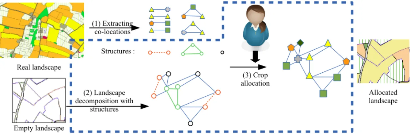
Our goal is to generate landscapes reproducing the land-use organization of some given real landscape. The general framework is illustrated in Figure 1. This paper focuses on steps in the dashed frame.
A landscape is formally represented by a graph G = hV, E, µ : V 7→ Σi where vertices of V represent plots, edges of E encode the adjacency of plots, Σ represents the crops (e.g. wheat, grassland, corn, etc.) and µ is an allocation func-tion that assigns to each plot one crop from Σ.
We assume that frequent co-locations are representative of a landscape. In order to replicate some landscape spatial or-ganization, the first step is, thus, the extraction of these co-locations from a real landscape. Algorithm gSpan [Yan and Han, 2002] has been adapted to extract frequent co-locations in the form of attributed sub-graphs. The spatial organization
Figure 1: Simulation process of land use in three stages: (1) co-location extraction; (2) an empty landscape is packed with the extracted structures; (3) the crops are allocated with respect to expert constraints.
of a co-location is extracted in a so-called structure that is represented as a non-attributed graph isomorphic to at least one co-location occurrence.
In a second step, the input bare landscape, i.e. a non-allocated plot graph, is divided into disjoint structure in-stances. The problem is to cover all vertices of the graph by non-overlapping instances.
Finally (third step), the process allocates crops to the plots of the new landscape, according to the crops in the co-location associated with the structure instances extracted from the original plot graph. In Figure 1, steps 2 and 3 are presented as sequential steps. Nonetheless, in our solving process they are solved simultaneously.
3
Graph packing with structures
This section introduces the specification of our specific prob-lem of graph packing with generic structures. Graph packing with well-known graph families – e.g. the set of complete graphs of size n, {Kn} – has been studied in graph theory
[Plummer and Lov´asz, 1986]. However, no algorithm has been proposed yet to solve efficiently the problem of graph packing with a set of structures having no specific topologi-cal properties.
Let G = hV, Ei be an unlabeled and undirected graph. Without loss of generality, we consider only connected graphs, i.e. with at least one path between two vertices. Pack-ing a non connected graph can be reduced to packPack-ing its con-nected components independently.
Let
S
be a set of connected graphs, called structures. Let ∼ (resp. ) denote the “isomorphic to” (resp. “not isomor-phic to ”) relation over graphs. We assume that ∀S1, S2∈S
, S1 S2.An instance I of a structure S = hVS, ESi ∈
S
in a graph G isa sub-graph hVI, EIi of G such that VI⊂ V , EI⊂ E and I ∼ S.
The set of instances is denoted
I
. The function s :I
7→S
maps instances to structures. A graph packing of G withS
is a set of instancesI
S ⊂I
such that each vertex of G isuniquely mapped to an instance vertex and conversely, each instance vertex is mapped to a single vertex in G. Moreover, if there exists an edge between two vertices in some instance
then there is an edge between the mapped vertices in G: • ∀I ∈
I
S, I = hVI, EIi ∧VI⊆ V ∧ EI⊆ E ∧ s(I) ∈S
• ∀v ∈ V, ∃!I ∈
I
S, I = hVI, EIi ∧ ∃!vI∈ VI, vI= v• ∀I = hVI, EIi ∈
I
S, ∀vI∈ VI, ∃!v ∈ V, vI= vThe size of a packing, denoted by |
I
|, is the number of in-stances inI
. The graph-packingI
of G is said to be optimal if its size is minimal.Note that in the general case, the graph-packing issue may have no solution or multiple solutions. We assume hereafter that
S
contains the singleton graph. Consequently, for any graph, there is at least one trivial packing solution consisting of singletons.Example We consider the graph G and the set of structures
S
illustrated in Figure 2.S
contains three structures: a pair (two connected vertices) displayed with a dashed edge, a tri-angle (three connected vertices) displayed with plain edges and the singleton graph. Figure 3 displays some correct pack-ings of G.4
Solving graph packing with ASP
ASP dates back from research on non monotonic logic and logic programming [Gelfond and Lifschitz, 1988]. An ASP program consists of Prolog-like rules l0
:-l1, . . . , lm, not lm+1, . . . , not ln, where each liis a literal. Such
a rule states that l0is proved to be true (l0 is in an answer
set) if l1, . . . , lmare true and one can not prove that lm+1. . . ln
are true. not stands for default negation. If the rule body
Figure 2: An instance of a graph packing problem: on the right, a graph to be packed with the three structures displayed on the left.
Figure 3: Six graph-packing solutions. Top-left: a packing with 6 instances (2 pairs and 4 singletons). Top-right: a pack-ing with 5 instances (3 pairs and 2 spack-ingletons). Bottom: four optimal packings by 4 instances (three solutions with 2 pairs, 1 singleton and 1 triangle; one solution with 2 triangles and 2 singletons).
is empty, l0 is a fact. A rule with an empty head
speci-fies an integrity constraint. Together with model minimal-ity, interpreting the program rules this way provides the sta-ble model semantics, see [Gelfond and Lifschitz, 1990] for details. Grounding on this theoretical work, efficient imple-mentations have been set up, cf. [Gebser et al., 2011]. An ASP system is the combination of a rich, yet simple, declara-tive modeling language with high-performance propositional solving capabilities relying on principles that led to fast SAT solvers. Given an ASP program, an ASP solver computes an-swer sets that are solutions of the encoded problem. To facil-itate the use of ASP in practice, several extensions have been brought to the language along time, such as choice, cardi-nality, aggregates, weight expressions and optimization state-ments. In the sequel, we rely on the input language of the ASP system clingo [Gebser et al., 2015].
The main objective of this paper is to show the effective-ness and flexibility of ASP for the graph-packing problem stated in section 3. The reminder of this section provides a first encoding for solving the graph packing problem in ASP. The next section will present how to break symmetries in or-der to improve the program efficiency.
4.1
Problem representation
The input graph to be packed, G, is encoded with predicates
vertex(X)stating thatXis a vertex andedge(X,Y)stating that there exists an edge between verticesXandYin graph G. The input structures S ∈
S
are encoded with atomsstructure (S)(Sis a structure of
S
),svertex (S,P)(Pis a vertex of structureS) andsedge(S,P,Q)(there exists an edge between vertexPand vertexQin structureS).A graph packing solution consists of non overlapping structure instances that cover all the graph vertices. Instances are encoded by predicates instance andmap describing the mapping of instance vertices to G vertices.instance(I,S)states thatIis an instance of structureSandmap(I, X, P)states that vertexPof instanceIis mapped to vertexXin G.
4.2
A generate and test program
Listing 1 introduces an ASP program for the packing prob-lem. It may be seen as a generate and test approach. The
Figure 4: Mapping structure instance vertices to graph ver-tices: Packing a graph (on the left) with structure instances (on the right). Each line between instance and graph vertices is coded by an atommap.
generation phase describes the space of all possible combina-tions of instances (lines 8-10) and, for each combination, it generates all possible mappings of instance vertices to graph vertices (lines 18-20). Line 1 ensures that graph edges are bidirectional since graphs are non-oriented.
1edge(X,Y) :− edge(Y,X). 2
3%additionnal graph features : graph size and stucture size 4 gsize (L) :− L = #count{ N : vertex(N) }.
5 ssize (S, L) :− L=#count{ N : svertex(S,N) }, structure (S) . 6
7% INSTANCE GENERATION
81 { instance (1, S) : structure (S) } 1.
9{ instance (I+1,S2) : S2>=S, structure(S2) } 1 :− 10 instance (I , S) , gsize (L), I<L.
11
12% The total number of instance vertices must be 13% equal to the number of vertices in the graph 14:− NI=#sum{ L,I : ssize (S,L), instance (I , S) }, 15 gsize (NG), NG!=NI.
16
17% MAPPING GENERATION
181 { map(I, X, 0) : vertex(X) } 1 :− instance (I , S) . 191 { map(I, Y, Q) : edge(X, Y) } 1 :−
20 instance (I , S) , sedge(S, P, Q), map(I, X, P). 21
22% an instance vertex must be mapped to a single 23% graph vertex
24:− map(I, P, X), map(I, P, Y), X<Y. 25% a graph vertex X must be mapped to a single 26% instance vertex
27:− map(I, X, ) , map(J, X, ) , I<J. 28:− map( , X, P), map( , X, Q), Q<P. 29% every graph vertex must be covered 30:− not map( , X, ) , vertex(X). 31
32%OPTIMIZATION
33nbinstances(L) :− L=#count{ I : instance (I , ) }. 34#minimize{ L : nbinstances(L) }.
Listing 1: Modeling graph-packing in ASP. See section 4.1 for predicate semantics.
Without a clever generation method, many equivalent in-stance sets are generated, differing only by the identifier as-signed to the different instances. To avoid this, we impose that instances are ordered. Structure and instance identifiers are represented by integers. Lines 8-10 state that the identi-fiers of instances are ordered with respect to the order of the identifiers of their related structure. In addition, the constraint in lines 14-15 imposes that the total number of vertices from
all the instances is equal to the number of vertices in the graph (given by predicategsize (N)).
The mapping described by mapatoms in lines 18-20 en-forces an isomorphism between each instance and some sub-graph of G: for each instance I containing a pair of map
atoms, if there is an edge between the vertices in the struc-ture associated withIthen an edge should exist between the mapped vertices in G.
To avoid the generation of (some) equivalent mappings, differing only by the identifier of mapped vertices, a structure S= hVS, ESi is modeled by a directed acyclic graph (DAG),
such that for any vertex v ∈ VS, there exists an oriented path
from a fixed root vertex v0to v. The set of oriented edges
defines a topological order for browsing efficiently the edges of this structure following a depth-first strategy.
Lines 18-20 implement such a depth-first search strategy in ASP. Line 18 states that the root vertex of instanceI(vertex
0) is mapped to a unique graph vertexX. Lines 19-20 state that each vertexQof some instance I, such that there is an edge fromPtoQand such thatPis mapped to graph vertex
X, is mapped to a graph vertexYsuch that there is an edge betweenXandY. Atomsmapgenerated this way define an isomorphism between VSand VI⊂ V , such that any edge of
the structure instance is associated with an edge in G, linking the mapped vertices of VI.
Lines 24-30 constrain the mapping by not allowing missing or unmapped edges. If there is no edge between two vertices
PandQin some structureS, then there should not exist any edge between the corresponding vertices in the graph. We use inequalitiesX<Y(logically equivalent toX!=Yin these cases), because X<Y leads to smaller grounding. Some of these constraints could be redundant, e.g. lines 24 and 28 (only one is mandatory), but improve computation times. Fi-nally, line 30 enforces that all the vertices of G are mapped.
The last part concerns optimization. Lines 33-34 keep only the optimal answer sets, i.e. the sets containing the minimum number of instances.
5
Breaking structure symmetries
Structure symmetries have a high impact on the combinatorial complexity of mapping since some structure can be mapped in several equivalent ways to a subgraph. Coping with such symmetries is a well known issue for ASP solvers [Drescher et al., 2011]. Symmetry breaking attempts to eliminate sym-metric parts of the search space. In the case of structures, this corresponds to finding bijective transformations on their set of nodes (e.g. rotations) such that the structure is left invari-ant by this transformation. Such transformations are called automorphisms. This section presents an ASP modeling of the search for automorphisms and the way they are used in graph packing for symmetry breaking.
5.1
Graph automorphisms
A permutation of a set Ω is a bijection from Ω to itself. For example, [5, 2, 6, 1, 4, 3] is a permutation of [1, 2, 3, 4, 5, 6]. A permutation can be represented as a composition of disjoint exchange cycles: (1 → 5 → 4) (3 → 6) = (1, 5, 4)(3, 6) for this example. Sym(Ω) is the set of all permutations of Ω.
Figure 5: Illustration of a structure with symmetries For an undirected graph G = hV, Ei, a graph automor-phism is a permutation of V that preserves adjacency. The set Aut(G) = {π ∈ Sym(V ) | π(E) = E} equipped with the composition of permutations ◦ forms a group that describes all possible symmetries. Using composition, this group may be generated from a few elements. For instance the group of symmetries for the graph in Figure 5 may be generated by 3 automorphisms: (0, 2), (3, 5), and (0, 3)(1, 4)(2, 5). A struc-ture has some symmetries if there is at least one non-identity permutation in the automorphism group.
Now, we relate automorphisms to the packing issue. Let G be a graph to be packed and S a structure. Let GS denote a
subgraph of G induced by an isomorphism φ between S and GS. Let π be an automorphism of S, then π ◦ φ is also an
iso-morphism between S and GS. In such a case, Listing 1 would
generate several answer sets corresponding to these automor-phisms for the same solution.
5.2
Finding automorphism symmetries in ASP
Our ASP encoding for finding automorphism symmetries is based on equitable partitions, as in the nauty program [McKay and Piperno, 2014]. An equitable partition consists of clusters of vertices, such that all vertices of a cluster have exactly the same number of neighbours in each cluster. An example of equitable partition is provided in Figure 5. Each cluster is displayed with a different color: each black vertex has 1 neighbor among grey vertices and 1 among white ver-tices and a similar observation can be done for white and grey vertices. Equitable partitions enable to reduce the search for automorphisms since it is a necessary condition for the cycles of the corresponding permutation. However, it is not suffi-cient and the graph isomorphism has to be verified (simple statement not shown in Listing 2).Listing 2 proposes an ASP encoding to search the space of equitable partitions and permutations (symsedgeis the sym-metric version ofsedge). This encoding is an elegant alterna-tive for the main task of nauty.
5.3
Breaking structure symmetries in ASP
Consider now a structure S with vertices VSand a graph G.
The mapping between S and G is represented by an isomor-phism φ. To each permutation π ∈ Aut(S) found by the pre-vious program may be associated some validity constraints to be satisfied by φ. Permutations are ordered partitions: the idea is to consider consecutive pairs of vertices in a cycle and to impose a compatible ordering in φ. This will reduce the number of admissible φ. More formally, an isomorphism φ will be “valid for a pair (u, v) in a permutation π ∈ Aut(S)” iff π has a cycle with two consecutive elements u and v and φ verifies u < v ⇒ φ(u) < φ(v).
Let π be a permutation that interchanges two elements, u and v and leaves the remaining elements unchanged. Then φ ◦
1%Partition : vertex N of structure S belongs to cluster B 21 { clust (S,B,N): svertex (S,B) } 1 :− svertex (S,N). 3 cluster (S,B) :− clust (S,B,N).
4
5%The number of neighbours of vertex N in cluster B is K 6nbneighb(S,N,B,K) :− svertex(S,N), cluster (S,B), 7 K=#count{ M: symsedge(S, M, N), clust(S,B,M) }. 8
9%K is a type of cluster B1 with respect to cluster B2 if an
element of B1 has K neighbours in B2
10type(S,B1,B2,K) :− clust (S,B1,M), nbneighb(S,M,B2,K). 11
12%Equitable partition : each cluster pair has a unique type 13:− 2 { type(S,B,X,L) }, cluster (S,B), cluster (S,X). 14
15%Permutation=Ordered partition: N2=succ(N1) in cluster B 161 { map(S,B,N1,N2): block(S,B,N2) } 1 :− block(S,B,N1).
Listing 2: Symmetry search through equitable partitions.
π and φ are two isomorphisms such that ∀w ∈ VS, w 6= u, w 6=
v, φ ◦ π(w) = φ(w), φ ◦ π(v) = φ(u) and φ ◦ π(u) = φ(v). Then, if u < v one and only one isomorphism will be valid for π.
The program looks for automorphisms that maximize the number of such constraining pairs. More generally, cycles larger than 2 may be constrained by more than one pair. How-ever, adding a validity constraint for each of the possible pairs may be unsatisfiable. The program looks for an automor-phism that maximizes the number of constraining pairs while leading to a valid isomorphism, i.e. an isomorphism valid for all constraining pairs.
In our example, (0, 2) and (3, 5) are two permutations for which φ is valid that will give two vertex constraints. In our ASP encoding of graph packing, validity constraints are en-coded by atomsordpair(S,P,Q)meaning that verticesPandQ
must be ordered in structureS. The following rule enforces the constraint in the program:
:− instance (I , S) , ordpair(S,P,Q), map(I, X, P), map(I, Y, Q), Y<=X.
ordpair/3 atoms are automatically generated from per-mutations. In our example, they are generated for pairs (0, 2), (3, 5), and also (1, 4), derived from (0, 2), (3, 5), and (0, 3)(1, 4)(2, 5).
6
Generating crop allocation
The graph-packing process decomposes the graph into small structures. The crop allocation process uses these structures to allocate crops to all vertices in the graph. An “allocated structure” is a structure instance where each vertex has been assigned a land use. Note that there may exist several allo-cated structures related to the same (bare) structure.
6.1
Crop allocation
The following predicates are introduced to implement crop allocation: attstruct (AS,S): ASis an allocated structure iso-morphic to structureS; attvertex (AS,P,A): vertexPof struc-ture AS is allocated with crop A; gvertexf (N,A): crop A is allocated to vertexN, at initialization; gvertex(N,A): cropA
1%fixed crops
2gvertex(N,A) :− gvertexf (N,A). 3 allocated (N) :− gvertexf (N,A). 4
5%free plots to allocate
61 { selectedAS(AS,I): attstruct (AS,S) } 1 :− 7 instance (I , S) .
8
9gvertex(N,A) :− attvertex (AS,P,A), selectedAS(AS,I) , 10 map(I,N,P), not allocated (N). 11:− gvertex(N,A), allocated (N), attvertex (AS,P,B), 12 map(I,N,P), selectedAS(AS,I) , instance (I , S) , A!=B.
Listing 3: Crop allocation.
1% No corn plot (8) neither wheat plot (7) close to forest (3)
2:− edge(X,Y), gvertex(X,8) , gvertex(Y,3) . 3:− edge(X,Y), gvertex(X,7) , gvertex(Y,3) . 4% Not less than 5 wheat plots
5ngvertex(L,OS) :− L=#count{ X: gvertex(X,OS) }. 6:− ngvertex(L,7) , L<5.
7% No additional plot with buildings (11) 8:− gvertex(X,11), not allocated (X). 9% A corn plot covers at least 5000 m2
10:− gvertex(X,8) , not allocated (X), surf (X,S), S<5000. 11% lusurf (C,A): A is the total area of plots with land use C 12lusurf (C,A) :− vertex(X), landuse(C),
13 A=#sum{ S: gvertex(X,C),surf(X,S) }. 14% At least 100000m2 is allocated with wheat 15:− lusurf (7, S) , S<100000.
Listing 4: Example of expert rules.
is allocated to graph vertexN, by crop allocation;selectedAS( AS,I): allocated structureASis associated with instanceI.
Crop allocation consists in generating atoms of thegvertex /2predicate. The land use of some plots, such as roads, build-ings, woods, can be static and should not be re-computed. Lines 2-3 of Listing 3 generategvertex/2atoms in such cases. Lines 9-10 generate gvertex/2 atoms in the other case. For each graph vertex, the crop is allocated with the crop associ-ated with the corresponding vertex in the allocassoci-ated structure. Lines 11-12 enforce consistency of initially allocated crops and mapped allocated structures: a crop allocated to some vertex must be identical to the crop initially allocated to this vertex, if any.
6.2
Modeling expert constraints
Beyond allocated structures modeling crop co-locations, ex-perts can add local or global constraints. Listing 4 illustrates the versatility of such constraints. Local constraints coerce or forbid the presence of some crops in the neighborhood of some plot. For instance, farmers used to not grow cereals close to forests to avoid damages by wild animals, such as boars or roes. This constraint is formulated in Line 2 of List-ing 4. Global constraints concern aggregates related to the whole crop allocation. Line 14 illustrates a global constraint on the overall surface allocated with wheat. The predicate
0 2 4 6 16 21 26 31 41 51 61 #node log(time) Progs ASP procedural
Figure 6: Computation time with respect to the number of graph vertices.
7
Experiments
The ASP solver clingo (version 4.5) [Gebser et al., 2011] was used on a desktop computer without parallelism for a quantitative evaluation of the efficiency of packing programs. 7*40 graphs1of size going from 16 to 61 vertices were ran-domly generated with a fixed edge density set to 1.2.
Figure 6 presents the computation times for packing ran-dom graphs with 10 structures containing at most 4 edges (5 vertices). The packing was solved with two methods: the “ASP” program (see Listing 1) without symmetry break-ing and a “procedural” program that implements a complete search with backtracking. The horizontal dotted line repre-sents the timeout of 10 min.
Figure 6 shows that computation time of the procedural approach is comparable with our approach for small graphs (sizes 16 and 21), but increases very quickly with the graph size. Beyond size 26, the procedural approach cannot solve the packing within the timeout period whereas our ASP en-coding does. For graphs of size larger than 31, ASP runs sev-eral orders of magnitude faster than the procedural program.
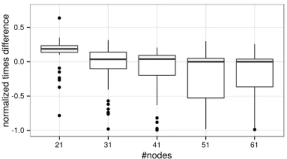
The efficiency of symmetry breaking was studied on pack-ing with a set of two structures: the spack-ingleton and the line of three vertices (S2). Figure 7 plots the normalized difference
of computation times with and without symmetry breaking. If this difference is above 0, taking symmetries into account is slower than ignoring them. This can be observed for small graphs. However, we can notice that the larger the graphs, the closer to 0 the mean is: symmetries do not significantly increase the computation time for large graphs. The negative skewness of the distribution of time differences shows that symmetry breaking is more efficient on larger graphs. It is worth noting that 12 problem instances2among the 200 in-stances could only be solved using symmetries.
The graph packing encoding has been integrated in a crop allocation tool. In this software, the expert provides a plot geometry in a standard geographical format (standard shape-files), a set of allocated structures and his own expert rules. These files are transformed into ASP facts. Then, the solver proposes crop allocations and, finally, an allocated landscape 1all programs and instances can be found at
https://sites.google.com/site/graphpacking/.
20 instances of size 21, 3 of size 31, 1 of size 41, 2 of size 51 and
6 of size 61. -1.0 -0.5 0.0 0.5 21 31 41 51 61 #nodes normalized times di ffer ence
Figure 7: Normalized time difference between ASP process-ing with/without symmetry breakprocess-ing.
is generated in a geographical format. Experiments have been done for 4 real landscapes containing up to 200 plots with edge densities of about 3. The software received a positive feedback from experts.
Figure 8 illustrates a practical application of crop alloca-tion on a landscape containing 45 plots. Roads, forests and buildings were allocated initially. The crop-allocated land-scape satisfies both the crop co-locations defined in allocated structures and expert rules. This landscape is one solution among all possible solutions. We can notice that wheat have been allocated only to the large plots that are not close to forests, as specified by expert rules.
Figure 8: Left: an empty agricultural plot with fixed land-uses. Right: an example of crop allocation satisfying the ex-pert rules (forest with tree glyphs, roads in dark grey, grass in hatched green, wheat in plain orange).
8
Conclusion
In this article, we have presented the problem of crop al-location with respect to co-al-locations. We have formalized the problem as a graph-packing problem which is known to be highly combinatorial. An ASP program has been pro-posed to solve the graph-packing problem and its perfor-mance has been assessed. Symmetry breaking was introduced to improve the efficiency of the basic solution. Solving the most difficult instances was significantly faster with symme-try breaking. This is highly valuable to a user who has to cope with large graphs and complex constraints. From a qualitative point of view, the resulting allocated landscapes are quite re-alistic. The realism can be easily enforced by adding expert rules stating local or global constraints. ASP is quite adapted for adding such background knowledge.
References
[Akplogan et al., 2013] M. Akplogan, S. de Givry, J-Ph. M´etivier, G. Quesnel, A. Joannon, and F. Garcia. Solv-ing the crop allocation problem usSolv-ing hard and soft con-straints. RAIRO - Operations Research, 47(2):151–172, 2013.
[Drescher et al., 2011] C. Drescher, O. Tifrea, and T. Walsh. Symmetry-breaking answer set solving. AI Communica-tions, 24(2):177–194, 2011.
[Gebser et al., 2011] M. Gebser, R. Kaminski, B. Kaufmann, M. Ostrowski, T. Schaub, and M. Schneider. Potassco: The Potsdam answer set solving collection. AI Communi-cations, 24(2):107–124, 2011.
[Gebser et al., 2015] M. Gebser, R. Kaminski, B. Kaufmann, M. Lindauer, M. Ostrowski, J. Romero, T. Schaub, and S. Thiele. Potassco User Guide, second edition, 2015. [Gelfond and Lifschitz, 1988] M. Gelfond and V. Lifschitz.
The stable model semantics for logic programming. In R. A. Kowalski and K. A. Bowen, editors, Proceedings of the Fifth International Conference on Logic Programming (ICLP), pages 1070–1080. MIT Press, 1988.
[Gelfond and Lifschitz, 1990] M. Gelfond and V. Lifschitz. Logic programs with classical negation. In Proceedings of the Seventh International Conference on Logic Program-ming (ICLP), pages 579–597, 1990.
[Lazrak et al., 2009] E. G. Lazrak, J.-F. Mari, and M. Benoit. Landscape regularity modelling for environmental chal-lenges in agriculture. Landscape Ecology, 25(2):169–183, 2009.
[Le Ber et al., 2009] F. Le Ber, C. Lavigne, K. Adamczyk, F. Angevin, N. Colbach, J-F. Mari, and H. Monod. Neutral modelling of agricultural landscapes by tessellation meth-ods - application for gene flow simulation. Ecological Modelling, 220:3536–3545, 2009.
[McKay and Piperno, 2014] B. D. McKay and A. Piperno. Practical graph isomorphism {II}. Journal of Symbolic Computation, 60(0):94–112, 2014.
[Plummer and Lov´asz, 1986] M. D. Plummer and L. Lov´asz. Matching theory. Elsevier, 1986.
[Schaller et al., 2012] N. Schaller, E. G. Lazrak, P. Martin, J.-F. Mari, C. Aubry, and M. Benot. Combining farm-ers decision rules and landscape stochastic regularities for landscape modelling. Landscape Ecology, 27(3):433–446, 2012.
[Yan and Han, 2002] X. Yan and J. Han. gSpan: Graph-based substructure pattern mining. In Proceedings of the International Conference on Data Mining, pages 721–724. IEEE, 2002.