HAL Id: inria-00261178
https://hal.inria.fr/inria-00261178v2
Submitted on 10 Mar 2008
HAL is a multi-disciplinary open access
archive for the deposit and dissemination of
sci-entific research documents, whether they are
pub-lished or not. The documents may come from
teaching and research institutions in France or
abroad, or from public or private research centers.
L’archive ouverte pluridisciplinaire HAL, est
destinée au dépôt et à la diffusion de documents
scientifiques de niveau recherche, publiés ou non,
émanant des établissements d’enseignement et de
recherche français ou étrangers, des laboratoires
publics ou privés.
Language for Intensive Multidimensional Signal
Processing
Pierre Boulet
To cite this version:
Pierre Boulet. Formal Semantics of Array-OL, a Domain Specific Language for Intensive
Multidimen-sional Signal Processing. [Research Report] RR-6467, INRIA. 2008, pp.33. �inria-00261178v2�
a p p o r t
d e r e c h e r c h e
0249-6399 ISRN INRIA/RR--6467--FR+ENG Thème COMFormal Semantics of Array-OL, a Domain Specific
Language for Intensive Multidimensional Signal
Processing
Pierre Boulet
N° 6467
Mars 2008
Centre de recherche INRIA Lille – Nord Europe Parc Scientifique de la Haute Borne
Processing
Pierre Boulet
*Thème COM — Systèmes communicants Équipe-Projet DaRT
Rapport de recherche n° 6467 — Mars 2008 — 30 pages
Abstract: In several application domains (detection systems, telecommunications, video processing, etc.) the applications deal with multidimensional data. These applications are usually embedded and subjected to real-time and resource con-straints. The challenge is thus to provide efficient implementations on parallel and distributed architectures. Array-OL has been designed specifically to handle this kind of intensive multidimensional signal processing applications. In this paper we present the language and its formal semantics. A subset of Array-OL, Static Array-OL, is defined that ensures the existence of a static scheduling. Finally, we discuss how to map and schedule an Array-OL application on a parallel and distributed architecture. Key-words: Array-OL, parallelism, data parallelism, multidimensional signal pro-cessing, formal semantics
*Laboratoire d’Informatique Fondamentale de Lille, Université des Sciences et Technologies de Lille,
au domaine du traitement du signal intensif
multidimensionnel
Résumé : Dans plusieurs domaines d’application (systèmes de détection, télé-communications, traitement vidéo, etc.) les applications manipulent des données multidimensionnelles. Elles sont de plus souvent embarquées et soumises à des contraintes de tems-réel et de ressources. Ainsi la difficulté est de construire des implémentations efficaces sur des architectures parallèles et distribuées. Array-OL a été conçu spécifiquement pour ces applications de taitement du signal intensif multidimensionnel. Nous proposons dans ce rapport une sémantique formelle pour Array-OL. Un sous-ensemble dArray-OL, Static Array-OL, est défini pour garantir l’existence d’un ordonnancement statique. Pour finir, nous discutons de la façon de placer et d’ordonnancer une application Array-OL sur une architecture parallèle et distribuée.
Mots-clés : Array-OL, parallélisme, parallélisme de données, traitement de signal multidimensionnel, sémantique formelle
1 Introduction
Computation intensive multidimensional applications are predominant in several application domains such as image and video processing or detection systems (radar, sonar). In general, intensive signal processing applications are multidimensional. By multidimensional, we mean that they primarily manipulate multidimensional data structures such as arrays. For example, a video is a 3D object with two spatial di-mensions and one temporal dimension. In a sonar application, one dimension is the temporal sampling of the echoes, another is the enumeration of the hydrophones and others such as frequency dimensions can appear during the computation. Actually, such an application manipulates a stream of 3D arrays.
Dealing with such applications presents a number of difficulties: • Only a few models of computation are multidimensional.
• The patterns of access to the data arrays are diverse and complex.
• Scheduling these applications with bounded resources and time is challenging, especially in a distributed context.
When dealing with parallel heterogeneous and constrained platforms and applica-tions, as it is the case of embedded systems, the use of a formal model of computation (MoC) is very useful. Edwards et al. [14] and more recently Jantsch and Sander [16] have reviewed the MoCs used for embedded system design. These reviews classify the MoCs with respect to the time abstraction they use, their support for concurrency and communication modeling. In our application domain there is little need for modeling state as the computations are systematic, the model should be data flow oriented. On the contrary, modeling parallelism, both task and data parallelism, is mandatory to build efficient implementations. More than a concrete representation of time, we need a way to express precedence relations between tasks. We focus on a high level of abstraction where the multidimensional data access patterns can be expressed. We do not look for a programming language but for a specification language allowing to deal with the multidimensional arrays easily. The specification has to be deadlock free and deterministic by construction, meaning that all feasible schedules compute the same result. In their review of models for parallel computation [32] Skillicorn and Talia classify the models with respect to their abstraction level. We aim for the second most abstract category which describes the full potential parallelism of the specification (the most abstract category does not even express parallelism). We want to stay at a level that is completely independent on the execution platform to allow reuse of the specification and maximal search space for a good schedule.
Table 1 presents a comparison of several languages (or models of computation) dedicated to signal processing. This comparison highlights the suitability of the various languages for intensive multidimensional signal processing. The main com-parison criteria are the allowed data structures (mono dimensional data flows or multidimensional arrays) and the expressivity of the access functions to these data structures. The class of applications these languages are able to deal with is also constrained by the control flow mechanisms they allow. As a common point, all these languages permit static scheduling in order to build efficient implementations. We have deliberately not included the dynamic variants of SDF or general purpose parallel programming languages though some of their features could be interesting in our context.
T a bl e 1: C omp ar ison of v ar iou s specific ation lan guages for si g nal pr ocessing Lang u ag e D at a T ype A cc e ss T y p e A ccess G en er ality C on tr o l S tr uct u res T ool sli d in g su b /o v er non // delays h ier ar chy modes su p por t w in do ws sampling to th e a xes SD F [26, 27 ] 1 D sub-arr ay -+ -P tolemy CSDF [2 ] 1 D sub-arr ay -+ -+ + S tr e a m-IT [33] 1 D sub-arr a y + + + + -S tr eamIT M D SDF [5 ,2 8] mu lti-D sub-arr a y -+ -+ -P tolemy GM D SDF [30 ,3 1] mu lti-D sub-arr a y -+ + + -WS DF [17 ,2 1] mu lti-D sub-arr a y + + -+ -? BLDF [2 2] mu lti-D sub-arr a y -+ -+ + + + Arr ay -OL [1 0, 11 ] cy c lic multi-D sub-arr ay + + + ext. + ext . G asp ar d Alph a [8, 25] pol yhedr a affi ne fu n ctions + + + + + -MM -Al p ha 1. C on cer n in g the data ty p e c o lumn, 1D mean s th at the sch edu ling c o n siders m o n o-d imen sio n al d ata st reams (th at may carr y mul tidimensional arr ay s as in S tr eamIT ), m u lti-D mean s th at th e se s d ata str eams ar e replaced b y mu ltidimen si on al arr ays , c y cli c mu lti-D mea ns that some dimens ion s of th e se mu lt idimen sio n al arr a y s may be cy c lic and poly hed ra m eans th at th e la ng u ag e han dles con v ex poly h edr a of in teger point s. 2. A + in a colu mn mean s th at the featur e is suppor ted, a -th at it is n ot an d ext . tha t it is supp o rted b y an e xtens ion to th e cor e lan guage .
Most of the compared languages are based on SDF or on its multidimensional extension, MDSDF. A detailed comparison of (G)MDSDF and Array-OL is available in [13]. As can be seen in the table, Array-OL is the only one able to deal with the following requirements of the application domain:
• Access to multidimensional arrays by regularly spaced sub-arrays. • Ability to deal with sliding windows.
• Ability to deal with cyclic array dimensions. • Ability to sub/over sample the arrays.
• Hierarchical specification to deal with complex systems.
The possibility to define sub-arrays that are not parallel to the axes is possible with Array-OL and GMDSDF though it may not be necessary for the multidimensional signal processing domain. In both cases it is a consequence of the generality of the approach. The control flow mechanisms are very limited in Array-OL. More complex mechanisms are introduced in section 5.2 which bring it on par with the other approaches. These extensions are not supported by the Array-OL tools yet.
An other language worth mentioning is Alpha, a functional language based on systems of recurrent equations [20]. Alpha is based on the polyhedral model, which is extensively used for automatic parallelization and the generation of systolic arrays. Alpha shares some principles with Array-OL:
• Data structures are multidimensional: union of convex polyhedra for Alpha and arrays for Array-OL.
• Both languages are functional and single assignment.
With respect to the application domain, arrays are sufficient and more easily handled by the user than polyhedra. Some data access patterns such as cyclic accesses are more easily expressible in Array-OL than in Alpha. And finally, Array-OL does not manipulate the indices directly but accesses the arrays through sub-arrays. In the one hand that restricts the application domain but in the other hand that makes it more abstract and more focused on the main difficulty of intensive signal processing applications: data access patterns.
The purpose of this paper is to present the Array-OL model of specification both in a pedagogical way and in a formal way. This is the first definition of a semantics for Array-OL. In section 2 we will define the core language along with its semantics by the way of a dependence relation. Then, in section 3, we will define some statically verifiable restrictions on the the language that will ensure that an application admits a static schedule. Next, in section 4, we will give some ideas on how to map and sched-ule such a static application on a parallel and distributed architecture. Sections 5 and 6 respectively present some extensions of Array-OL to extend the application domain and the available tools. Section 7 summarizes and concludes this paper.
2 Core language
As a preliminary remark, Array-OL is only a specification language, no rules are specified for executing an application described with Array-OL, but a static scheduling can be easily computed using this description.
2.1 Principles
The initial goal of Array-OL is to give a mixed graphical-textual language to express multidimensional intensive signal processing applications. As said before, these applications work on multidimensional arrays. The complexity of these applications does not come from the elementary functions they combine, but from their combina-tion by the way they access the intermediate arrays. Indeed, most of the elementary functions are sums, dot products or Fourier transforms, which are well known and often available as library functions. The difficulty and the variety of these intensive signal processing applications come from the way these elementary functions access their input and output data as parts of multidimensional arrays. The complex access patterns lead to difficulties to schedule these applications efficiently on parallel and distributed execution platforms. As these applications handle huge amounts of data under tight real-time constraints, the efficient use of the potential parallelism of the application on parallel hardware is mandatory.
From these requirements, we can state the basic principles that underly the language:
• All the potential parallelism in the application has to be available in the specifi-cation, both task parallelism and data parallelism.
• Array-OL is a data dependence expression language. Only the true data depen-dences are expressed in order to express the full parallelism of the application, defining the minimal order of the tasks. Thus any schedule respecting these dependences will lead to the same result. The language is deterministic. • It is a single assignment formalism. No data element is ever written twice. It
can be read several times, though. This single assignment constraint is at the scalar level, not at the array level. Array-OL can be considered as a first order functional language.
• Data accesses are done through sub-arrays, called patterns.
• The language is hierarchical to allow descriptions at different granularity levels and to handle the complexity of the applications. The dependences expressed at a level (between arrays) are approximations of the precise dependences between the array elements.
• The spatial and temporal dimensions are treated equally in the arrays. In particular, time is expanded as a dimension (or several) of the arrays. This is a consequence of single assignment.
• The arrays are seen as tori. Indeed, some spatial dimensions may represent some physical tori (think about some hydrophones around a submarine) and some frequency domains obtained by FFTs are toroidal.
The semantics of Array-OL is that of a first order functional language manipulating multidimensional arrays. It is not a data flow language but can be projected on such a language.
As a simplifying hypothesis, the application domain of Array-OL is restricted. No complex control is expressible and the control is independent of the value of the data. This is realistic in the given application domain, which is mainly data flow. Some efforts to couple control flows and data flows expressed in Array-OL have been done in [23] but are outside the scope of this paper.
2.2 Basic definitions
The usual model for dependence based algorithm description is the dependence graph where nodes represent tasks and edges dependences. Various flavors of these graphs have been defined. The expanded dependence graphs represent the task parallelism available in the application. In order to represent complex applications, a common extension of these graphs is the hierarchy in which a node can itself be a graph. Array-OL builds upon such hierarchical dependence graphs and adds repetition nodes to represent the data-parallelism of the application.
2.2.1 Syntax
Precisely, an Array-OL application is a set of tasks connected through ports. The tasks are equivalent to mathematical functions reading data on their input ports and writing data on their output ports. The tasks are of three kinds: elementary, compound and repetition. An elementary task is atomic (a black box), it can come from a library for example. A compound is a dependence graph whose nodes are tasks connected via their ports. A repetition is a task expressing how a single sub-task is repeated.
All the data exchanged between the tasks are arrays. These arrays are multidi-mensional and are characterized by their shape, the number of elements on each of their dimension1. A shape will be noted as a column vector or a comma-separated tuple of values indifferently. Each port is thus characterized by the shape and the type of the elements of the array it reads from or writes to. As said above, the Array-OL model is single assignment. One manipulates values and not variables. Time is thus represented as one (or several) dimension of the data arrays. For example, an array representing a video is three-dimensional of shape (width of frame, height of frame, frame number).
Remark. There is no relation between the shapes of the inputs and the outputs of a task. So a task can read two two-dimensional arrays and write a three-dimensional one. The creation of dimensions by a task is very useful, a very simple example is the FFT which creates a frequency dimension.
We will illustrate the rest of the presentation of Array-OL by an application that scales an high definition TV signal down to a standard definition TV signal. Both signals will be represented as a three dimensional array.
2.2.2 Formal definition
Definition 1 (tasks). The set of tasks,T is the disjoint union2of the set of elementary tasks,E , the set of compound tasks, C , and the set of repetitive tasks, R.
T = E ∪∗C ∪∗R (1)
Each task ofT is characterized by an interface.
Definition 2 (interface). The interface of a task lists its input and output ports, their name, direction, type and shape. It is defined by the interface function.
interface :T → P (String × {IN,OUT} × Type × Shape) (2)
1A point, seen as a 0-dimensional array is of shape (), seen as a 1-dimensional array is of shape (1), seen
as a 2-dimensional array is of shape¡1
1¢, etc.
2The mathematical notations used in this paper are consistent with those of MathWorld (http:// mathworld.wolfram.com/).
Property 1. The names of the ports of a task must be all different. ∀((p, dp,τp, sp), (q, dq,τq, sq)) ∈ interface(T ),
p = q ⇒ (p,dp,τp, sp) = (q,dq,τq, sq) (3)
A port, (p, dp,τp, sp), of a given task can thus be uniquely identified by its name, p.
Notation. We note t .p the port of name p of task t .
Definition 3 (shape). The shape spof port t .p belongs to the set
Shape =[
n∈N
(N∗∪ ∞)n . (4)
Notation. We note dim(sp) the dimension of the shape vector.
The type system (Type, ∼=) for the elements of the arrays can be arbitrarily complex. Type is the set of available types and ∼= is the unification relation. This relation means that a data of typeτ can be used in a context that waits for type τ0if and only ifτ ∼= τ0.
For the intensive signal processing application domain, we can rely on a very simple one where the type unification relation, ∼=, is defined by the equality.
Definition 4 (array type). The type of the data consumed or produced through port (p, dp,τp, sp) is a multidimensional array of shape spof data elements of typeτp. It is a collection of elements Ap= {Ap[i] :τp, 0 ≤ i < sp} where d = dim(sp) and a :τ
means that a is of typeτ. This typing function on the elements is thus extended to the multidimensional arrays as A :τ[s] which reads as “the array A is a multidimensional array of shape s of elements of typeτ”. The type unification relation between arrays is thus defined by
τ[s] ∼= τ0[s0] ⇔ τ ∼= τ0and s = s0 (5)
Notation. A :τ means that array A is of type τ, in the same way, p : τ means that the data consumed or produced by the port p have the typeτ.
Notation. The element of index i of array A is written A[i].
Let us define a few derived functions that will help the explanation below. Definition 5 (inputs and outputs). The function inputs returns the set of input ports of a task.
inputs :T → P (String × {IN,OUT} × Type × Shape) t 7→ {(p,dp,τp, sp) ∈ interface(t) | dp= IN}
(6)
The function outputs returns the set of output ports of a task. outputs :T → P (String × {IN,OUT} × Type × Shape)
t 7→ {(p,dp,τp, sp) ∈ interface(t) | dp= OUT}
(7)
2.2.3 Semantics
As said above, the semantics of Array-OL is data dependence based. The data depen-dence relation has to give a strict partial ordering on the calls to the elementary tasks to define an executable algorithm.
Horizontal Filter
(1920, 1080, ∞) (720, 1080, ∞)
Vertical Filter
(720, 1080, ∞) (720, 480, ∞)
Figure 1: Top-level Compound of the Downscaler
Definition 6 (calling context). The definition of the calling context, notedΓ, will be precised in the following sections. It contains a path up to the main task call. From this calling context, we can relate the data consumed and produced by a particular call to a task to the data consumed and produced by the caller task up to the data of the main task call.
Notation. Γ::t is the call to the task t in the calling context Γ.
Notation. Γ::t.p is the data consumed or produced by the port p of the call to the task t in the calling contextΓ.
Definition 7 (application). A call ;::t to a task t in an empty context defines an application. This application has input data and output data.
Remark. Actually, a classical intensive signal processing application receives data from sensors and provides data to actuators. It can thus be modelled in Array-OL as an application taking its inputs from infinite arrays and producing infinite arrays. In these arrays, the succession of samples in time is represented by an explicit infinite dimension of the arrays.
In order to define the data dependence relation, →, between the calls to the elementary tasks, we need to define a dependence relation between array elements. The dependence relation, , between the elements of the arrays will be precisely defined below in function of the kind of task t (elementary, compound or repetitive). Notation (Dependence relations).
is the dependence relation between array elements.
→ is the dependence relation between calls to elementary tasks.
Definition 8 (dependence relation between calls to elementary tasks). The depen-dence relation between calls to elementary tasks, →, is derived from the precise dependence relation between array elements as follows. For two calls to two elemen-tary tasks,Γ::t and Γ0::t0,Γ::t → Γ0::t0if and only if there exists an element o in one of
the arrays produced byΓ::t and an element i0in one of the arrays consumed byΓ0::t0 such that o i0.
2.3 Elementary tasks
An elementary task is a black box mathematical function. It has no internal state and so it computes its results depending only on its input data and not on its calling context or any internal state.
Definition 9 (dependence relation between array elements for an elementary task). If t ∈ E , then, for any calling context, Γ, for any input array, Γ::t.piwith pi∈ inputs(t ), for any output array,Γ::t.powith po∈ outputs(t ),
∀(i , o) ∈ Γ::t .pi× Γ::t .po, i o . (8)
2.4 Task parallelism
2.4.1 Syntax
The task parallelism is represented by a compound task. The compound description is a simple directed graph. Each node represents a task and each edge a dependence connecting two ports of unifiable types.
2.4.2 Formal definition
Definition 10 (compound task). A compound graph is a directed graph. ∀c ∈ C , c = (N , E) where N ⊂ T
and E ⊂ {outputs(t) × inputs(t0), (t , t0) ∈ N2} (9) Property 2. The non connected ports of the nodes of the graph are the ports of the compound with an optional renaming. Formally, there exists a bijectionπ defined by
π : interface(c) → [ n∈N interface(n) \ [ (p,p0)∈E {p, p0} (p, dp,τp, sp) 7→(q,dq,τq, sq) where dq= dp,τq= τp and sq= sp (10)
Property 3. The ports connected by an edge must be unifiable:
∀(p, p0) ∈ E , p : τ, p0:τ0⇒ τ ∼= τ0 (11) Property 4. If the compound c is called in the contextΓ, the nodes of the graph are called in the contextΓ::c. The graph thus defines some equalities on the data:
∀p ∈ interface(c), Γ::c.p = Γ::c::π(c.p) (12)
∀(p, p0) ∈ E ,Γ::c::p = Γ::c::p0 (13)
2.4.3 Semantics
The dependence relation between the elements of the input arrays and output arrays of a call,Γ::c, to a compound task, c = (N,E) is derived by transitivity along the edges of the graph from the dependence relations between the input and output array elements of the nodes of the graph.
Definition 11 (dependence relation between array elements inside a compound). For a calling context,Γ, for a compound c = (N,E), for two arrays Γ::c::t.p and Γ::c::t0.p0,
with (t , t0) ∈ N2, p ∈ inputs(t) and p0∈ outputs t0, ∀(i , o) ∈ Γ::c::t .p × Γ::c::t0.p0, i o ⇔ ∃n ∈ N, ∃(tk)0≤k<n∈ Nn, ∀k ∈ N, 0 ≤ k < n, ∃pINk ∈ inputs(tk), ∃p OUT k ∈ outputs(tk), pIN0 = p and pOUTn−1 = p0, ∀k ∈ N, 1 < k < n − 1, ¡tk.pOUTk , tk+1.pINk+1¢ ∈ E, ∀k ∈ N, 0 ≤ k < n, ∃ek∈ Γ::c::tk.pINk , en= o ∈ Γ::c::tn−1.pn−1OUT, e0= i and ∀k ∈ N, 0 ≤ k < n, ek ek+1 (14)
This definition is meaningful thanks to property 4. Indeed, for all k ∈ N,0 ≤ k < n, ekis an element of an input array ofΓ::c::tkand ek+1is an element of an output array of the same callΓ::c::tk.
Definition 12 (dependence relation between array elements for a compound). For a calling context,Γ, the dependence relation between the elements of an input array, Γ::c.pi, with pi∈ inputs(c) and those of an output array, Γ::c.po, with po∈ outputs(c) is derived from definition 11 through the projectionπ following property 4. Indeed, ∀i ∈ Γ::c.pi, ∀o ∈ Γ::c.po, i ∈ Γ::c::π(c.pi) and o ∈ Γ::c::π(c.po), and definition 11 applies.
Remark. There may be several paths in the graph that lead to a dependence between array elements in a compound.
2.4.4 Example
We will study as a running example a downscaler from high definition TV to standard definition TV. Fig. 1 describes the top level compound. The tasks are represented by named rectangles, their ports are squares on the border of the tasks. The shape of the ports is written as a tuple of positive numbers or ∞. The dependences are represented by arrows between ports.
There is usually a limitation on the shapes: there can be at most one infinite dimension by array. Most of the time, this infinite dimension is used to represent the time, so having only one is quite sufficient.
Each execution of a task reads data from one array on each of its inputs and writes data to one array per output. It’s not possible to read from more than one array per port to write to one output. The graph is a dependence graph, not a data flow graph. So it is possible to schedule the execution of the tasks just with the compound description. But it’s not possible to express the data parallelism of our applications be-cause the details of the computation realized by a task are hidden at this specification level.
2.5 Data parallelism
A data-parallel repetition of a task is specified in a repetition task. The basic hypoth-esis is that all the repetitions of this repeated task are independent. They can be scheduled in any order, even in parallel3. The second one is that each instance of the
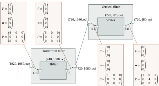
Horizontal filter (1920, 1080, ∞) (720, 1080, ∞) (240, 1080, ∞) Hfilter (13) (3) F = 1 0 0 o = 0 0 0 P = 8 0 0 0 1 0 0 0 1 F = 1 0 0 o = 0 0 0 P = 3 0 0 0 1 0 0 0 1
Figure 2: Horizontal Filter Repetitive Task
repeated task operates with sub-arrays of the inputs and outputs of the repetition. For a given input or output, all the sub-array instances have the same shape, are composed of regularly spaced elements and are regularly placed in the array. This hypothesis enables a compact representation of the repetition and is coherent with the application domain of Array-OL which describes very regular algorithms. 2.5.1 Syntax
As these sub-arrays are conform (same shape), they are called patterns when con-sidered as the input arrays of the repeated task and tiles when concon-sidered as a set of elements of the arrays of the repetition task. In order to give all the information needed to create these patterns, a tiler is associated to each array (i.e. each edge). A tiler is able to build the patterns from an input array, or to store the patterns in an output array. It describes the coordinates of the elements of the tiles from the coordinates of the elements of the patterns. It contains the following information:
• F : a fitting matrix.
• o: the origin of the reference pattern (for the reference repetition). • P : a paving matrix.
Visual representation of a repetition task The shapes of the arrays and patterns are, as in the compound description, noted on the ports. The repetition space indicating the number of repetitions is defined itself as an multidimensional array with a shape. Each dimension of this repetition space can be seen as a parallel loop and the shape of the repetition space gives the bounds of the loop indices of the nested parallel loops. An example of the visual description of a repetition is given in Fig. 2 by the horizontal filter repetition from the downscaler. The tilers are connected to the dependences linking the arrays to the patterns. Their meaning is explained below.
(0) (1) (2)
F =µ30 
spattern=¡3¢
There are here 3 elements in this tile because the shape of the pattern is (3). The indices of these elements are thus (0), (1) and (2). Their position in the tile relatively to thereference pointare thusF· (0) =¡0
0¢ ,F· (1) =
¡3 0¢ ,F· (2) =
¡6 0¢.
Figure 3: Fitting Example with a Stride
Building a tile from a pattern From a reference element (ref) in the array, one can extract a pattern by enumerating its other elements relatively to this reference ele-ment. The fitting matrix is used to compute the other elements. The coordinates of the elements of the pattern (ei) are built as the sum of the coordinates of the reference
element and a linear combination of the fitting vectors as follows
∀ i, 0 ≤ i < spattern, ei= ref + F · i mod sarray (15)
where spatternis the shape of the pattern, sarrayis the shape of the array and F the
fitting matrix.
In the examples of fitting matrices and tiles from Fig. 3, 4 and 5, the tiles are drawn from a reference element in a 2D array. The array elements are labeled by their index in the pattern, i, illustrating the formula ∀i,0 ≤ i < spattern, ei=ref+F· i. Thefitting
vectorsconstituting the basis of the tile are drawn from thereference point.
¡1 0 ¢ ¡0 1 ¢ ¡1 1 ¢ ¡0 2 ¢ ¡1 2 ¢ ¡0 0 ¢ F =µ10 01 ¶ spattern=µ23 
The pattern is here two-dimensional with 6 elements. Thefitting matrixbuilds a compact rectangular tile in the array.
Figure 4: Compact Fitting Example
A key element one has to remember when using Array-OL is that all the dimen-sions of the arrays are toroidal. That means that all the coordinates of the tile ele-ments are computed modulo the size of the array dimensions. The more complex examples of tiles of Fig. 6 and 7are drawn from a fixed reference element (o as ori-gin in the figure) in fixed size arrays, illustrating the formula ∀i,0 ≤ i < spattern, ei=
o+F· i modsarray.
Paving an array with tiles For each repetition, one needs to design the reference elements of the input and output patterns. A similar scheme as the one used to enumerate the elements of a pattern is used for that purpose.
¡1 0 ¢ ¡0 1 ¢ ¡1 1 ¢ ¡0 2 ¢ ¡1 2 ¢ ¡0 0 ¢ F =µ20 11 ¶ spattern=µ23 
This last example illustrates how the tile can be sparse, thanks to the¡2
0¢ fitting vector, and
non parallel to the axes of the array, thanks to the¡1
1¢ fitting vector.
Figure 5: Non Parallel to the Axes Fitting Example
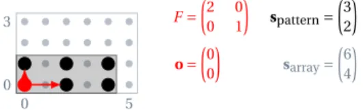
0 5 0 3 F =µ20 01 ¶ spattern=µ32 ¶ o =µ00 ¶ sarray=µ64 
Figure 6: A Sparse Tile Aligned on the Axes of the Array
0 5 0 3 F =µ11 ¶ spattern=¡6¢ o =µ20 ¶ sarray=µ64 
The pattern is here mono-dimensional, thefittingbuilds a diagonal tile that wraps around the array because of the modulo.
Figure 7: Oblique Fitting
0 9 0 4 r = (0) 00 9 4 r = (1) 00 9 4 r = (2) 00 9 4 r = (3) 00 9 4 r = (4) F =µ10 ¶ spattern=¡10¢ o =µ00 ¶ sarray=µ105 ¶ P =µ01 ¶ srepetition=¡5¢
This figure represents the tiles for all the repetitions in the repetition space, indexed byr. Thepaving vectorsdrawn from the originoindicate how the coordinates of the reference elementrefrof the current tile are computed. Here the array is tiled row by row.
Figure 8: Simple Paving Example
The reference elements of the reference repetition are given by the origin vector, o, of each tiler. The reference elements of the other repetitions are built relatively to this one. As above, their coordinates are built as a linear combination of the vectors
0 8 0 7 r =¡0 0 ¢ 0 8 0 7 r =¡1 0 ¢ 0 8 0 7 r =¡2 0 ¢ 0 8 0 7 r =¡0 1 ¢ 0 8 0 7 r =¡1 1 ¢ 0 8 0 7 r =¡2 1 ¢ F =µ1 0 0 1 ¶ spattern=µ34 ¶ o =µ00 ¶ sarray=µ98 ¶ P =µ30 04 ¶ srepetition=µ32 
Figure 9: A 2D Pattern Tiling Exactly a 2D Array
0 9 0 4 r =¡0 0 ¢ 0 9 0 4 r =¡1 0 ¢ 0 9 0 4 r =¡2 0 ¢ 0 9 0 4 r =¡0 1 ¢ 0 9 0 4 r =¡1 1 ¢ 0 9 0 4 r =¡2 1 ¢ 0 9 0 4 r =¡0 2 ¢ 0 9 0 4 r =¡1 2 ¢ 0 9 0 4 r =¡2 2 ¢ F =µ10 01 ¶ spattern=µ53 ¶ o =µ00 ¶ sarray=µ105 ¶ P =µ01 30 ¶ srepetition=µ33 
0 31 0 17 r =¡0 0 ¢ F =µ10 ¶ spattern=¡13¢ o =µ00 ¶ sarray=µ3218 ¶ P =µ80 01 ¶ srepetition=µ 418 ¶ HFilter 0 11 0 17 r =¡0 0 ¢ F =µ10 ¶ spattern=¡3¢ o =µ00 ¶ sarray=µ1218 ¶ P =µ30 01 ¶ srepetition=µ 418 ¶ 0 31 0 17 r =¡1 0 ¢ HFilter 0 11 0 17 r =¡1 0 ¢ 0 31 0 17 r =¡2 5 ¢ HFilter 0 11 0 17 r =¡2 5 ¢
of the paving matrix as follows
∀ r, 0 ≤ r < srepetition, refr= o + P · r mod sarray (16)
where srepetitionis the shape of the repetition space, P the paving matrix and sarraythe
shape of the array. Fig. 8, 9 and 10 give some examples.
Summary We can summarize all these explanations with one formula. For a given repetition index r, 0 ≤ r < srepetitionand a given index i, 0 ≤ i < spatternin the pattern,
the corresponding element in the array has the following coordinates: o + (P F ) ·µri
mod sarray , (17)
where sarrayis the shape of the array, spatternis the shape of the pattern, srepetitionis
the shape of the repetition space, o is the coordinates of the reference element of the reference pattern, also called the origin, P is the paving matrix whose column vectors, called the paving vectors, represent the regular spacing between the patterns, F is the fitting matrix whose column vectors, called the fitting vectors, represent the regular spacing between the elements of a pattern in the array.
Some constraints on the number of rows and columns of the matrices can be derived from their use. The origin, the fitting matrix and the paving matrix have a number of rows equal to the dimension of the array; the fitting matrix has a number of columns equal to the dimension of the pattern4; and the paving matrix has a number of columns equal to the dimension of the repetition space.
Linking the inputs to the outputs by the repetition space The previous formulas explain which element of an input or output array one repetition consumes or pro-duces. The link between the inputs and outputs is made by the repetition index, r. For a given repetition, the output patterns (of index r) are produced by the repeated task from the input patterns (of index r). These pattern elements correspond to array elements through the tiles associated to the patterns. Thus the set of tilers and the shapes of the patterns and repetition space define the dependences between the elements of the output arrays and the elements of the input arrays of a repetition. As stated before, no execution order is implied by these dependences between the repetitions.
To illustrate this link between the inputs and the outputs, we show in Fig. 11 several repetitions of the horizontal filter repetition. In order to simplify the figure and as the treatment is made frame by frame, only the first two dimensions are represented5. The sizes of the arrays have also been reduced by a factor of 60 in each dimension for readability reasons.
2.5.2 Formal definition
Definition 13 (repetition). A repetition task, r ∈ R, is defined by r = (t,sR,C ) where
t ∈ T is the repeated task, sR∈ Shape is the shape of the repetition space and C ⊂
4Thus if the pattern is a single element viewed as a zero-dimensional array, the fitting matrix is empty
and noted as (). The only element of a tile is then its reference element. This can be viewed as a degenerate case of the general fitting equation where there is no index i and so no multiplication F · i.
5Indeed, the third dimension of the input and output arrays is infinite, the third dimension of the
repetition space is also infinite, the tiles do not cross this dimension and the only paving vector having a non null third element is³00
1
´
interface(r )×interface(t)×Θ is the set of repetition connectors (see definition below) between the ports of r and those of t .Θ is the set of triplets composed of an integer matrix, an integer vector and an integer matrix.
Definition 14 (repetition connector). A repetition connector, ((p, dp,τp, sp), (q, dq,τq, sq),θ) ∈
interface(r ) × interface(t) × Θ, defines the tiling of the arrays handled by the port p of the repetition task by the arrays handled by the calls to the repeated task t through the port q. The tiler,θ = (F,o,P) ∈ Ndim(sp)×dim(sq)× Ndim(sp)× Ndim(sp)×dim(sR), is
com-posed of a fitting matrix, F , an origin vector, o, and a paving matrix, P .
Property 5. To be allowed in a repetition task definition, a repetition connector, ((p, dp,τp, sp), (q, dq,τq, sq),θ), has to verify
dp= dq, (18)
dp= IN ⇒ τp∼= τq, (19)
dp= OUT ⇒ τq∼= τp. (20)
Definition 15 (calling context in a repetition). If r = (t,sR, T ) ∈ R is called in the
calling contextΓ, then it defines the following calls to t indexed by the repetition index, r:
{Γ::r ::t[r],∀r ∈ Ndim(sR), 0 ≤ r < s
R} . (21)
Property 6. The definitions of the repetition connectors imply some equalities on the data manipulated by the callsΓ::r and Γ::r ::t[r]:
∀((p, dp,τp, sp), (q, dq,τq, sq), (F, o, P )) ∈ T, ∀i ∈ Ndim(sq), 0 ≤ i < s q, Γ::r.p · o + (P F )µri ¶ mod sp ¸ = Γ::r ::t [r].q[i] . (22) 2.5.3 Semantics
Definition 16 (dependence relation between array elements for a repetition). For a calling context,Γ, for an input array, Γ::r.piwith (pi, dpi,τpi, spi) ∈ inputs(r ), for an
output array,Γ::r.powith (po, dpo,τpo, spo) ∈ outputs(r ),
∀ji∈ Ndim¡spi ¢ , 0 ≤ ji< spi, ∀jo∈ Ndim(spo),0 ≤ jo< spo,Γ::r.pi[ii] Γ::r.po[io] ⇔ ∃r ∈ Ndim(sR), 0 ≤ r < s R, ∃((pi, dpi,τpi, spi), (qi, dqi,τqi, sqi), (Fi, oi, Pi)) ∈ T, ∃((po, dpo,τpo, spo), (qo, dqo,τqo, sqo), (Fo, oo, Po)) ∈ T, ∃ii∈ Ndim¡sqi ¢ , 0 ≤ ii< sqi, ∃io∈ Ndim(sqo),0 ≤ io< sqo, ji= oi+ (PiFi) µ r ii ¶ mod spi, jo= oo+ (PoFo) µ r io ¶ mod spo, Γ::r ::t[r].qi[ii] Γ::r ::t[r].qo[io] . (23)
2.6 Summary
We have provided for each kind of task, elementary, compound and repetitive, their formal definition and the construction of the dependence relation between array elements. By induction, this dependence relation is now fully defined and the depen-dence relation between the calls to the elementary tasks can be derived following definition 8.
In the following section, we will propose some construction rules and the way to statically verify them that ensures that this dependence relation between the calls to the elementary tasks admits a static schedule.
3 Enforcing Static Schedulability
All the specifications following the definition of Array-OL are not valid. Some may not even respect the basic hypotheses of the language such as single assignment. Others may have cycles in the dependence relations and thus lead to deadlocks. We will give here some easily and statically verifiable rules that will ensure that the specification is statically schedulable.
3.1 Requirements for schedulability
An application is statically schedulable if the dependence relation between the calls to the elementary tasks is a strict partial order. Indeed, any schedule following this order computes the same values from the same input. Some tools to help the user schedule its application onto a distributed and parallel architecture are proposed in section 4.2.
We propose the following restrictions on the language to ensure this static schedu-lability:
• The shapes of all the arrays are known values, not parameters.
• The output arrays of a task are always fully produced if the input arrays are fully defined.
∀Γ, ∀t ∈ T , ∀po∈ outputs(t ), ∀o ∈ Γ::t .po,
∃pi∈ inputs(t ), ∃i ∈ Γ::t .pi, i o (24) • There is no cycle in the graph of a compound task.
We will call Static Array-OL this restricted language.
For each kind of task, we will give a way to statically verify these conditions and prove by induction that the dependence relation between the calls to the elementary tasks depending whose calling context includes the considered task is a strict partial order.
3.2 Elementary tasks
By definition 9, the elementary tasks fully produce their outputs by reading their inputs. For any callΓ::e to an elementary task e, there is only one elementary task call including this context:Γ::e. Thus the dependence relation is trivialy a strict partial order.
3.3 Compound tasks
Let c = (N ,E) be a compound task. For any calling context Γ, the induction hypoth-esis is that for any task t ∈ N , the dependence relation → between the calls to the elementary tasks in the contextΓ::c::t is a strict partial order. Further more, all these tasks callsΓ::c::t produce theirs outputs completely.
The restriction proposed above is that there is no cycle in the dependence graph. A cycle is such a graph is the usual graph theory cycle notion on a graph G = (N ,E0) derived from (N , E ) whose nodes are N and where there is an edge between two nodes if and only if there is an edge in E between some ports of these two nodes. The graph G is thus a directed acyclic graph and defines a strict partial order on its nodes. Following definition 11, the dependence relation between the calls to the elemen-tary tasks in the contextΓ::t is the hierarchical composition of the strict partial orders defined by the sub-tasks in N and the strict partial order defined by G. It is easy to check that this composition defines a strict partial order.
3.4 Repetition tasks
For repetitive tasks, we have to check that the output arrays are fully produced. As the repetition is fully parallel, there is no dependence between two elementary tasks calls coming from different repetitions. The induction property is thus trivially respected. A direct consequence of the full production rule is that a repetition has to tile exactly its output arrays. In other words each element of an output array has to belong to exactly one tile. Verifying this can be done by using polyhedral computations using a tool like SPPoC6[4].
To check that all the elements of an output array have been produced, one can check that the union of the tiles spans the array. The union of all the tiles produced by a repetition connector c = (p, q,(F,o,P)) can be built as the set of points e(r,i)verifying
the following system of (in)equations
Sc= 0 ≤ r < srepetition
refr= o + P · r mod sarray
0 ≤ i < spattern
e(r,i)= refr+ F · i mod sarray
. (25)
As several repetition connectors, Sc1, . . . , Sck, can produce elements of the same array, the set of points produced by the repetition is given by the union of these sets, S =Sk
i =1Sci. We then build the difference between the array and this set S and check that it is empty. The union and difference of such sets are done in one operation each from the Polylib7(that is included in SPPoC) and testing if the resulting set is empty is done by looking for an element in this set using a call to the PIP8[15] solver that is also included in SPPoC. These operations are possible because, as the shapes are known values, the system of inequations is equivalent to a system of affine equations defining unions of linearly bounded lattices with which SPPoC, the Polylib and PIP work.
To check that no point is computed several times in an output array, we first have to check that any two repetition connectors producing values on the same port do not produce the same indices. This is done by checking the emptyness of
6http://www.lifl.fr/west/sppoc/ 7http://icps.u-strasbg.fr/polylib/ 8http://www.piplib.org/
the intersections of the Sci and Sc0
i sets as above. Then one has to check that the points produced by two tiles of a repetition connector do not overlap. This is done by building the following set of points, e, (intersection of two tiles) verifying the following system of (in)equations
0 ≤ r < srepetition
refr= o + P · r mod sarray
0 ≤ i < spattern
e = refr+ F · i mod sarray
0 ≤ r0< srepetition
refr0= o + P · r0mod sarray
0 ≤ i0< spattern
e = refr0+ F · i0mod sarray
. (26)
If this set is empty, then no two tiles overlap and each computed element is computed once. To check the emptiness of this set, the same technique as above can be used: to call PIP. As above, the above system of inequations is equivalent to a system of affine equations, thus solvable by PIP.
With these two checks, one can ensure that all the elements of the output arrays are computed exactly once and so that the single assignment is respected.
3.5 Static Array-OL Scheduling
By induction, using the results of the previous sections, the Static Array-OL language is statically schedulable. Indeed, any schedule that respects the strict partial order → between the calls to the elementary tasks of an application will compute the same result without any deadlock. We will study in the next section how the projection of an Array-OL specification to a distributed and parallel execution platform can be made.
4 Projection onto an execution model
The Array-OL language expresses the minimal order of execution that leads to the correct computation. This is a design intension and lots of decisions can and have to be taken when mapping an Array-OL specification onto an execution platform: how to map the various repetition dimensions to time and space, how to place the arrays in memory, how to schedule parallel tasks on the same processing element, how to schedule the communications between the processing elements?
4.1 Space-time mapping
One of the basic questions one has to answer is: What dimensions of a repetition should be mapped to different processors or to a sequence of steps? To be able to answer this question, one has to look at the environment with which the Array-OL specification interacts. If a dimension of an array is produced sequentially, it has to be projected to time, at least partially. Some of the inputs could be buffered and treated in parallel. On the contrary, if a dimension is produced in parallel (e.g. by different sensors), it is natural to map it to different processors. But one can also group some repetitions on a smaller number of processors and execute these groups sequentially. The decision is thus also influenced by the available hardware platform.
Horizontal filter (1920, 1080, ∞) (720, 1080, ∞) (240, 1080, ∞) Hfilter (13) (3) F = 1 0 0 o = 0 0 0 P = 8 0 0 0 1 0 0 0 1 F = 1 0 0 o = 0 0 0 P = 3 0 0 0 1 0 0 0 1 Vertical filter (720, 1080, ∞) (720, 480, ∞) (720, 120, ∞) Vfilter (14) (4) F = 0 1 0 o = 0 0 0 P = 1 0 0 0 9 0 0 0 1 F = 0 1 0 o = 0 0 0 P = 1 0 0 0 4 0 0 0 1 The interesting array is the intermediate (720, 1080, ∞) array that is produced by tiles of 3
elements aligned along the first dimension and consumed by tiles of 14 elements aligned on the second dimension.
Figure 12: Downscaler Before Transformation
production patterns consumption patterns
0 11 0 17 r =¡0 0 ¢ 0 11 0 17 r =¡0 0 ¢
Figure 13:601-th of the First Two Dimensions and Suppression of the Infinite Dimen-sion of the Intermediate (720, 1080, ∞) Array of the Downscaler
(1920, 1080, ∞) (720, 480, ∞) (240, 120, ∞) (14, 13) (3, 4) F = 0 1 1 0 0 0 o = 0 0 0 P = 8 0 0 0 9 0 0 0 1 F = 1 0 0 1 0 0 o = 0 0 0 P = 3 0 0 0 4 0 0 0 1 Horizontal filter (14, 13) (3, 14) (14) Hfilter (13) (3) F =µ01 ¶ o =µ00 ¶ P =µ10 ¶ F =µ10 ¶ o =µ00 ¶ P =µ01 ¶ Vertical filter (3, 14) (3, 4) (3) Vfilter (14) (4) F =µ01 ¶ o =µ00 ¶ P =µ10 ¶ F =µ01 ¶ o =µ00 ¶ P =µ10 
A hierarchical level has been created that is repeated (240, 120, ∞) times. The intermediate array between the filters has been reduced to the minimal size that respects the depen-dences. If the inserted level is executed sequentially and if the two filters are executed on different processors, the execution can be pipelined.
Figure 14: Downscaler After Fusion
It is a strength of Array-OL that the space-time mapping decision is separated from the functional specification. This allows to build functional component libraries for reuse and to carry out some architecture exploration with the least restrictions possible.
Mapping compounds is not specially difficult. The problem comes when mapping repetitions. This problem is discussed in details in [1] where the authors study the projection of Array-OL onto Kahn process networks [18, 19]. The key point is that some repetitions can be transformed to flows. In that case, the execution of the repetitions is sequentialized (or pipelined) and the tiles are read and written as a flow of tokens (each token carrying a tile).
4.2 Transformations
A set of Array-OL code transformations has been designed to allow to adapt the application to the execution, allowing to choose the granularity of the flows and a simple expression of the mapping by tagging each repetition by its execution mode: data-parallel or sequential.
These transformations allow to cope with a common difficulty of multidimen-sional signal processing applications: how to chain two repetitions, one producing an array with some paving and the other reading this same array with another paving? To better understand the problem, let us come back to the downscaler example where the horizontal filter produces a (720, 1080, ∞) array row-wise 3 by 3 elements and the
(1920, 1080, ∞) (720, 480, ∞) (120, ∞) (14, 1920) (720, 4) F = 0 1 1 0 0 0 o = 0 0 0 P = 0 0 9 0 0 1 F = 1 0 0 1 0 0 o = 0 0 0 P = 0 0 4 0 0 1 Horizontal filter (14, 1920) (720, 14) (240, 14) Hfilter (13) (3) F =µ01 ¶ o =µ00 ¶ P =µ09 10 ¶ F =µ10 ¶ o =µ00 ¶ P =µ30 01 ¶ Vertical filter (720, 14) (720, 4) (240, 3) Vfilter (14) (4) F =µ01 ¶ o =µ00 ¶ P =µ30 10 ¶ F =µ01 ¶ o =µ00 ¶ P =µ30 10 
The top-level repetition now works with tiles containing full rows of the images. Less parallelism is expressed at that level but as the images arrive in the system row by row, the buffering mechanism is simplified and the full parallelism is still available at the lower level.
Figure 15: Downscaler After Fusion and Change-Paving
vertical filter reads it column-wise 14 elements by 14 elements with a sliding overlap between the repetitions as shown on Fig. 12 and 13.
In order to be able to project this application onto an execution platform, one possibility is to make a flow of the time dimension and to allow pipelining of the space repetitions. A way to do that is to transform the application by using the fusion transformation to add a hierarchical level. The top level can then be transformed into a flow and the sub-level can be pipelined. The transformed application is described on Fig. 14.
This form of the application takes into account internal constraints: how to chain the computations. Now, the environment tells us that a TV signal is a flow of pixels, row after row. We can now propose a new form of the downscaler application taking that environment constraint into account by extending the top-level patterns to include full rows. Such an application could look like the description in Fig. 15.
A full set of transformations (fusion, tiling, change paving, collapse) described in [12] allows to adapt the application to the execution platform in order to build an efficient schedule compatible with the internal computation chaining constraints, those of the environment and the possibilities of the hardware. A great care has been taken in these transformations to ensure that they do not modify the semantics of the specifications. They only change the way the dependences are expressed in different hierarchical levels but not the precise element to element dependences.
5 Extensions
Around the core Array-OL language, several extensions have been proposed recently. We will give here the basic ideas of these extensions and pointers to references where the reader can go into details.
5.1 Inter-Repetition dependences
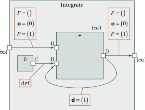
One of the lacks of Array-OL is the impossibility to specify delays. We have chosen to represent them as uniform dependences between tiles produced by a repeated task and tiles consumed by this repeated task. The simplest example is the discrete integration shown on Fig. 16.
Integrate (∞) (∞) 0 () (∞) + () () () F =¡ ¢ o =¡0¢ P =¡1¢ F =¡ ¢ o =¡0¢ P =¡1¢ def d =¡1¢
Figure 16: Inter-Repetition Example: Discrete Integration
Here the patterns (and so the tiles) are single points. The uniform dependence vector d = (1) tells that repetition r depends on repetition r − d(= r − (1)) by adding the result of the addition of index r − (1) to the input tile r. This is possible because the output pattern and input pattern linked by the inter-repetition dependence connector have the same shape. To start the computation, a default value of 0 is taken for repetition 0.
Formally, for a call to a repetition task,Γ::r an inter-repetition dependence con-nects an output port poof the repeated task t with one of its input ports pi. The shape of these connected ports must be identical. The connector is tagged with a dependence vector d that defines the dependence distance between the dependent repetitions. This dependence is uniform, that means identical for all the repetitions. When the source of a dependence is outside the repetition space, a default value is used. This default value is defined by a connector tagged with “def” which can be connected to an input port of r or to an output port of a constant task called inside r . Such a constant task is a task without inputs. Its outputs are thus constant arrays.
This dependence adds the following equalities on the data elements of the re-peated tasks. ∀r ∈ Ndim(sR), 0 ≤ r < s R, 0 ≤ r + d < sR, ∀i ∈ Ndim(spi), 0 ≤ i < sp i, Γ::r ::t[r].pi[i] = Γ::r ::t[r − d].po[i]. (27)
If the default connector is connected to port di of task r , then ∀r ∈ Ndim(sR), 0 ≤ r < s R, r + d < 0 or ,sR≤ r + d ∀i ∈ Ndim(spi), 0 ≤ i < sp i, Γ::r ::t[r].pi[i] = Γ::r.di[i], (28) else, it is connected to port doof a task c and
∀r ∈ Ndim(sR), 0 ≤ r < s
R, r + d < 0 or ,sR≤ r + d
∀i ∈ Ndim(spi), 0 ≤ i < sp i,
Γ::r ::t[r].pi[i] = Γ::r ::c.do[i]. (29) These equalities are propagated by the relation to define some dependences between the elements of the output arrays. This is the only way to define dependence relations between elements of a same array.
In order to allow a static scheduling of such an application, the output tiles must not overlap (as in Static Array-OL) and a schedule must exist for the repetition. If several such inter-repetition dependences are defined for a repetition, one can use the results on the scheduling of loop nests with uniform dependences [6, 7] to statically verify that a schedule exist and build one.
5.2 Control modeling
In order to model mixed control flow, data flow applications, Labbani et al. [23, 24] have proposed to use the mode automata concept. An adaptation of this concept to Array-OL is necessary to couple an automaton and modes described as Array-OL tasks corresponding to the states of that automaton.
A controlled task is a switch allowing to select one task according to a special “mode” input. All the selectable tasks must have the same interface. An automaton task produces a 1D array of values that will be used as mode inputs of a controlled task. A repetition task allows to associate the mode values to a repetition of a controlled task.
Both the inter-repetition and the control modeling extensions can be used at any level of the hierarchy, thus allowing to model complex applications. The Array-OL transformations still need to be extended to deal with these extensions.
6 Tools
Several tools have been developed using the Array-OL language as specification language. Gaspard Classic9[9] takes as input an Array-OL specification, allows the user to apply transformations to it, and generates multi-threaded C++ code allowing to execute the specification on a shared memory multi-processor computer.
The Gaspard210co-modeling environment [3] aims at proposing a model-driven environment to co-design intensive computing systems-on-chip. It proposes a UML profile to model the application, the hardware architecture and the allocation of the application onto the architecture. The application metamodel is based on Array-OL
9http://www.lifl.fr/west/gaspard/classic.html 10http://www.lifl.fr/west/gaspard/
with the inter-repetition dependence and control modeling extensions. The hardware metamodel takes advantage of the repetition mechanism proposed by Array-OL to model repetitive hardware components such as SIMD units, multi-bank memories or networks-on-chip. The allocation mechanism also builds upon the Array-OL constructs to express data-parallel distributions. The Gaspard2 tool is built as an Eclipse11plugin and mainly generates SystemC code for the co-simulation of the modeled system-on-chip. It also includes an improved transformation engine.
Two smaller tools are also available12: a simulation [13] of Array-OL in PtolemyII [29] and Array-OL example, a pedagogical tool helping to visualize repetitions in 3D. And to be complete, we have to mention that Thales has developed its own internal tools using Array-OL to develop radar and sonar applications on multiprocessor platforms.
Acknowledgment
The author would like to thank all the members of the west team of the LIFL for their very useful comments on drafts of this paper.
7 Conclusion
We have presented in this paper the Array-OL language and its formal semantics. This language is dedicated to specify intensive signal processing applications. It al-lows to model the full parallelism of the application: both task and data parallelisms. Array-OL is a single assignment first order functional language manipulating multidi-mensional arrays. It focuses on the expression of the main difficulty of the intensive signal processing applications: the multidimensional data accesses. It proposes a mechanism able to express at a high level of abstraction the regular tilings of the arrays by data-parallel repetitions.
We have formally defined the language and its semantics by the way of a depen-dence relation between the calls to the elementary tasks. A restricted Static Array-OL language has been defined that allows static scheduling. We have then discussed how to map and schedule an Array-OL application onto a parallel and distributed archi-tecture and proposed some extensions to the language to add control flow expression mechanism.
As an Array-OL specification describes the minimal ordering of the computations, its space-time mapping has to be done taking into account constraints that are not expressed in Array-OL: architectural and environmental constraints. A toolbox of code transformations allows to adapt the application to its deployment environment. Future works include extending this toolbox to handle the control extensions and automating the allocation process of an application on a distributed heterogeneous platform in the Gaspard2 co-modeling environment.
References
[1] Abdelkader Amar, Pierre Boulet, and Philippe Dumont. Projection of the Array-OL specification language onto the Kahn process network computation model.
11http://www.eclipse.org/
In International Symposium on Parallel Architectures, Algorithms, and Networks, Las Vegas, Nevada, USA, December 2005.
[2] G. Bilsen, M. Engels, R. Lauwereins, and J.A. Peperstraete. Cyclo-static data flow. In International Conference on Acoustics, Speech, and Signal Processing., Detroit, MI, USA, May 1995.
[3] Pierre Boulet, Cédric Dumoulin, and Antoine Honoré. From MDD concepts to experiments and illustrations, chapter Model Driven Engineering for System-on-Chip Design. ISTE, International scientific and technical encyclopedia, Hermes science and Lavoisier, September 2006.
[4] Pierre Boulet and Xavier Redon. SPPoC : manipulation automatique de polyè-dres pour la compilation. Technique et Science Informatiques, 20(8):1019–1048, 2001. (In French).
[5] Michael J. Chen and Edward A; Lee. Design and implementation of a multidi-mensional synchronous dataflow environment. In 1995 Proc. IEEE Asilomar Conf. on Signal, Systems, and Computers, 1995.
[6] Alain Darte and Yves Robert. Constructive methods for scheduling uniform loop nests. IEEE Trans. Parallel Distributed Systems, 5(8):814–822, 1994.
[7] Alain Darte, Yves Robert, and Frédéric Vivien. Scheduling and Automatic Par-allelization. Birkhauser Boston, 2000. http://www.birkhauser.com/detail. tpl?isbn=0817641491.
[8] Florent de Dinechin, Patrice Quinton, and Tanguy Risset. Structuration of the alpha language. In Programming Models for Massively Parallel Computers, pages 18–24, Berlin, Germany, October 1995.
[9] Jean-Luc Dekeyser, Philippe Marquet, and Julien Soula. Video kills the radio stars. In Supercomputing’99 (poster session), Portland, OR, November 1999. (http://www.lifl.fr/west/gaspard/).
[10] Alain Demeure and Yannick Del Gallo. An Array Approach for Signal Processing Design. In Sophia-Antipolis conference on Micro-Electronics (SAME 98), France, October 1998.
[11] Alain Demeure, Anne Lafarge, Emmanuel Boutillon, Didier Rozzonelli, Jean-Claude Dufourd, and Jean-Louis Marro. Array-OL : Proposition d’un formalisme tableau pour le traitement de signal multi-dimensionnel. In Gretsi, Juan-Les-Pins, France, September 1995. (In French).
[12] Philippe Dumont. Spécification Multidimensionnelle pour le traitement du sig-nal systématique. Thèse de doctorat (PhD Thesis), Laboratoire d’informatique fondamentale de Lille, Université des sciences et technologies de Lille, Decem-ber 2005.
[13] Philippe Dumont and Pierre Boulet. Another multidimensional synchronous dataflow: Simulating Array-OL in ptolemy II. Research Report RR-5516, INRIA, March 2005.
[14] S. Edwards, L. Lavagno, E. A. Lee, and A. Sangiovanni-Vincentelli. Design of embedded systems: Formal models, validation, and synthesis. Proc. of the IEEE, 85(3), year 1997.
[15] P. Feautrier. Parametric integer programming. RAIRO Recherche Opérationnelle, 22(3):243–268, 1988.
[16] Axel Jantsch and Ingo Sander. Models of computation and languages for em-bedded system design. IEE Proceedings on Computers and Digital Techniques, 152(2):114–129, March 2005. Special issue on Embedded Microelectronic Sys-tems; Invited paper.
[17] Jürgen Teich Joachim Keinert, Christian Haubelt. Windowed synchronous data flow. Technical Report Co-Design-Report 02, 2005, Department of Computer Science 12, Hardware-Software-Co-Design, University of Erlangen-Nuremberg, Am Weichselgarten 3, D-91058 Erlangen, Germany, 2005.
[18] Gilles Kahn. The semantics of a simple language for parallel programming. In Jack L. Rosenfeld, editor, Information Processing 74: Proceedings of the IFIP Congress 74, pages 471–475. IFIP, North-Holland, August 1974.
[19] Gilles Kahn and David B. MacQueen. Coroutines and networks of parallel processes. In B. Gilchrist, editor, Information Processing 77: Proceedings of the IFIP Congress 77, pages 993–998. North-Holland, 1977.
[20] Richard M. Karp, Raymond E. Miller, and Shmuel Winograd. The organization of computations for uniform recurrence equations. J. ACM, 14(3):563–590, July 1967.
[21] Joachim Keinert, Christian Haubelt, and Jürgen Teich. Modeling and analysis of windowed synchronous algorithms. In International Conference on Acoustics, Speech and Signal Processing (ICASSP), pages III–892– III–895, 2006.
[22] Dong-Ik Ko and Shuvra S. Bhattacharyya. Modeling of block-based dsp systems. The Journal of VLSI Signal Processing, 2005.
[23] Ouassila Labbani, Jean-Luc Dekeyser, Pierre Boulet, and Éric Rutten. Introduc-ing control in the gaspard2 data-parallel metamodel: Synchronous approach. International Workshop MARTES: Modeling and Analysis of Real-Time and Em-bedded Systems (in conjunction with 8th International Conference on Model Driven Engineering Languages and Systems, MoDELS/UML 2005), October 2005. [24] Ouassila Labbani, Jean-Luc Dekeyser, Pierre Boulet, and Éric Rutten. UML2 profile for modeling controlled data parallel applications. In FDL’06: Forum on Specification and Design Languages, Darmstadt, Germany, September 2006. [25] Hervé Le Verge, Christophe Mauras, and Patrice Quinton. The alpha language
and its use for the design of systolic arrays. The Journal of VLSI Signal Processing, 3(3):173–182, September 1991.
[26] E. A. Lee and D. G. Messerschmitt. Static scheduling of synchronous data flow programs for digital signal processing. IEEE Trans. on Computers, January 1987. [27] E. A. Lee and D. G. Messerschmitt. Synchronous Data Flow. Proc. of the IEEE,


![[PDF] Formation du langage PHP : Les expression régulières | Formation informatique](data:image/gif;base64,R0lGODlhAQABAIAAAP///wAAACH5BAEAAAAALAAAAAABAAEAAAICRAEAOw==)