Changements de sélection de l’habitat du campagnol à
dos roux à la suite d’une coupe forestière
Mémoire
Julie Martineau
Maîtrise en Biologie
Maître ès sciences (M.Sc.)
Québec, Canada
© Julie Martineau, 2014
iii
RÉSUMÉ
Ce projet visait à évaluer les changements à court terme de sélection d’habitat du campagnol à dos roux (Myodes gapperi) à la suite d’une coupe forestière. La répartition des campagnols a été observée avant la coupe, puis une semaine, un mois et 1-2 ans après la coupe. Nous avons aussi évalué les processus biologiques pouvant expliquer cette répartition. Même si l’abondance des campagnols est demeurée similaire entre la coupe et la forêt durant le premier mois, l’importance relative des processus biologiques influençant cette abondance a varié. Une semaine après la coupe, la sélection d’habitat ne dépendait pas de la densité de la population. Un mois après la coupe, la compétition par interférence jouait un rôle majeur dans la sélection de l’habitat des campagnols. Finalement, nos travaux supportent l’hypothèse qu’une dynamique source-puits serait responsable de l’important déclin d’abondance des campagnols dans la coupe observé 1-2 ans après la perturbation.
v
ABSTRACT
The goal of this study was to assess short-term changes in habitat selection by red-backed voles (Myodes gapperi) following forest harvesting. The spatial distribution of voles was observed before harvesting, and then a week, a month and 1-2 years after harvest. We also evaluated the ecological processes that can explain observed temporal changes in vole distribution. Although vole abundance remained similar between clearcuts and uncut forests during the first month, different ecological processes appeared to influence vole distribution. A week after harvesting, there was no evidence that habitat selection influenced the distribution of vole populations. A month after harvesting, interference competition exerted a strong influence on habitat selection of red-backed voles, hence on their distribution. Finally, our study supports the hypothesis that source-sink dynamics would be responsible for the strong decline in vole abundance observed in clearcuts 1-2 years after harvesting.
vii
TABLE DES MATIÈRES
RÉSUMÉ ... iii
ABSTRACT ... v
TABLE DES MATIÈRES ... vii
LISTE DES TABLEAUX ... ix
LISTE DES FIGURES ... xi
LISTE DES ANNEXES ... xiii
REMERCIEMENTS ... xv
AVANT-PROPOS ... xvii
INTRODUCTION ... 1
Répartition animale et théorie de sélection d’habitat ... 3
Objectif de l’étude ... 7
Le campagnol à dos roux comme espèce à l’étude ... 8
CHAPITRE PRINCIPAL ... 9
Processes driving short-term temporal dynamics of small mammals in human-disturbed environments ... 9 Résumé ... 10 Abstract... 11 Introduction ... 12 Methodology... 16 Results ... 22 Discussion... 27 Acknowledgements ... 31 References ... 31 CONCLUSION GÉNÉRALE ... 37 Originalité du projet ... 42 Perspectives ... 43 BIBLIOGRAPHIE GÉNÉRALE ... 45 ANNEXE ... 53
ix
LISTE DES TABLEAUX
Table 1: Parameter estimates of GLMM models that assessed the short-term impact of logging on the abundance (individuals/100 trap-nights) of four categories of red-backed voles in the black spruce boreal forest of the Côte-Nord region of Québec (Canada) in 2012 and 2013. Treatment (Trt) refers to uncut vs cut stands, whereas Time contrasts before logging with one week and one month after logging.……….. 25
xi
LISTE DES FIGURES
Figure 1 : a) Exemple de relation entre l’aptitude phénotypique et la densité des individus dans deux habitats de qualité différente, A étant de meilleure qualité que B. b) Isodar issu du tracé de la densité de l'habitat A en fonction de la densité de l'habitat B. (adapté de Morris (1988))..………..………...……….... 4 Figure 2: Locations of the three sectors sampled over this study. For each sector, the number indicates the number of sites sampled……….... 19 Figure 3: Schematic view of one site corresponding to a pair of transects crossing the two habitats (cut and uncut stand) in boreal forest. The small rectangles correspond to live-trap locations. ……….... 20 Figure 4. Abundances of red-backed voles (juveniles and adults combined) between cut and old-growth forest, and the estimated isodar estimated: a) before, and b) less than a week, c) one month and d) one-two years after the logging. The dotted line corresponds to 1:1 line and the solid line is the regression line (displayed only if significant) ………..……. 26 Figure 5. Abundances of adult red-backed voles between cut and uncut old-growth forest, and the estimated isodar curves a) before b) less than a week and c) one month after the logging. Black dotted line in each figure corresponds to 1:1 line and the solid line corresponds to a regression (displayed only if significant).………...………….. 27 Figure 6. Abundances of juvenile red-backed voles between cut and uncut old-growth forest, and the estimated isodar curves a) before b) less than a week and c) one month after the logging. Black dotted line in each figure corresponds to 1:1 line and the solid line corresponds to a regression (displayed only if significant).………...……….. 28
xiii
LISTE DES ANNEXES
Annexe 1. Isodars contrasting abundance of red-backed voles in uncut and cut stand in the black spruce boreal forest of northeastern Quebec (Canada). Results of linear regression are presented for all sampling, adults and juveniles and separated into time. Significant regressions at 0.05 levels are marked with an asterisk. Slopes which were significantly upper to 0. Upper (UCI) and lower (LCI) 95% confidence intervals are included for both slopes (S) and intercept (I)... 48 Annexe 2: Relationship between the number of locations and the resulting average home range size (ha), as estimated based on telemetry of adult red-backed voles in the black spruce boreal forest of the Côte-Nord region of Québec (Canada) in 2012 and 2013……..49
xv
REMERCIEMENTS
Tout d’abord, j’aimerais remercier mon directeur de recherche, Daniel Fortin, pour m’avoir fait confiance pour ce projet. Malgré les épreuves, j’ai adoré mes deux étés sur le terrain. Merci d’avoir pris le temps de répondre à mes questions et de m’avoir orientée dans la bonne direction.
Je remercie également David Pothier, mon codirecteur, qui a toujours été disponible et rapide à répondre à mes questions. Merci d’avoir pris le temps de corriger mes travaux et d’avoir donné des conseils.
Merci à Steeve Côté et Gwenaël Beauplet pour leurs idées sur mon proposé de recherche. Merci aussi à André Desrochers et Marcel Darveau pour leurs commentaires sur mon mémoire.
Un merci tout spécial à Angélique Dupuch qui a su me guider dès mon arrivée à l’été 2012, alors que j’étais une petite étudiante récemment diplômée du Baccalauréat. Elle a été présente lorsque j’en ai eu besoin et j’ai beaucoup appris avec elle.
Merci aux nombreuses personnes qui sont venues m’aider sur le terrain, sans qui l’acquisition des données n’aurait pas été possible. En 2012, j’ai eu l’aide précieuse d’Hélène Le Borgne qui a su me guider dans mon projet. Merci à mes deux assistants de 2012, Michaël Leblanc et Antoine Daigneault, à qui nous leur en avons demandé beaucoup. Merci à Orphé Bichet, Chrystel Losier et Angélique Dupuch qui sont venues nous prêter main-forte pour terminer l’été en beauté. En 2013, j’ai eu la chance d’avoir trois assistants qui ont travaillé fort : Caroline Bergeron, Félix Gagnon et Antoine Boudreau-Leblanc. Je garde de beaux souvenirs de ces deux étés.
Merci à Produit forestier Résolu et Boisaco de m’avoir accueillie sur leurs parterres de coupe et dans leur camp forestier. Mes demandes étaient particulières, mais ils ont tout fait pour répondre à celles-ci. Aussi, je m’en voudrais de ne pas remercier les gens que j’ai
xvi
côtoyés pendant deux étés dans les camps forestiers. Merci aux cuisiniers, cuisinières, concierges, préposés, contremaîtres, surintendants, techniciens forestiers, camionneurs, etc. Ils m’ont chaleureusement accueillie parmi eux, j’étais la « petite souris » du camp.
Un gros merci également à Philippe Goulet pour son aide dans la planification des travaux de terrain. Il a facilité la communication avec les compagnies forestières, il a obtenu les cartes de coupe, il a fourni une aide précieuse pendant les premiers jours de terrain et, surtout, il nous a tous fait bien rire avec ses expressions.
Mon expérience à la maîtrise n’aurait pas été la même sans mes collègues de laboratoire. J’aimerais donc remercier tous les membres du laboratoire qui ont été là pendant mes deux années de maîtrise. Mes collègues de bureau, Orphé Bichet, Hélène Le Borgne et Chrystel Losier, j’ai adoré vous côtoyer tous les matins et vous raconter mes histoires souvent non pertinentes de ma fin de semaine ou de la soirée d’avant. Caroline Gagné, tu as su me motiver à persévérer et, surtout, tu as été une source de déconnage. Merci aux autres membres du laboratoire Jerod Merkle, Marie Sigaud et Olivia Tardy qui ont su être disponibles lorsque j’avais des interrogations. Vous m’avez tous encouragée, donné des conseils et répondu à mes questions. Grâce à vous, j’ai passé de merveilleux moments.
Finalement, le plus gros des remerciements revient à ma famille qui m’a appuyée pendant toute la durée de mes études à Québec. J’ai des parents formidables qui sont fiers de moi et fiers d’avoir une biologiste dans la famille. Sans leur soutien, je ne serais pas où je suis maintenant.
xvii
AVANT-PROPOS
Ce mémoire de maîtrise vise à évaluer et comprendre les changements de répartition à court terme du campagnol à dos roux à la suite d’une coupe forestière. Ce mémoire contient trois parties : une introduction générale, un chapitre présenté sous la forme d’un article scientifique rédigé en anglais et une conclusion générale. En tant que première responsable du projet et étant donné ma contribution au projet (récolte des données, compilations et analyses des données, écriture du mémoire et de l’article), je serai premier auteur de l’article. Les chercheurs qui sont coauteurs de l’article sont:
- Daniel Fortin, directeur de maîtrise et professeur au département de biologie de l’Université Laval. Il a contribué à l’élaboration du projet, au développement de la méthode statistique et à la rédaction de l’article.
- David Pothier, codirecteur de maîtrise et professeur au département de foresterie de l’Université Laval. Il a contribué à l’élaboration du projet et à la rédaction et révision de l’article.
Le chapitre principal servira de base à un article qui sera éventuellement publié dans un journal scientifique international en anglais.
1
INTRODUCTION
Les perturbations, qu’elles soient naturelles ou anthropiques, peuvent changer fortement la qualité de l’habitat de plusieurs espèces animales (Huston, 1994) en modifiant la structure et la composition de l’habitat. Cela peut notamment se traduire par une modification de l’abondance et du type de ressources disponibles pour les animaux, ce qui peut avoir un impact immédiat sur la répartition et l’abondance des animaux. Ces changements vont donc également influencer directement la dynamique des populations animales (Gill et al., 1996, Larson et al., 2004). Par exemple, Jacob (2003) a observé qu’un mois après le labourage de terres agricoles qui a provoqué la perte du couvert protecteur, la densité, le taux de survie, le taux de reproduction et le recrutement des campagnols des champs (Microtus arvalis) étaient réduits. Toutefois, la densité est revenue à son niveau initial au cours de la saison de récolte suivante. En revanche, des perturbations majeures peuvent avoir des conséquences à plus long terme. Par exemple, les passereaux et les oiseaux de rivage sont restés absents de l’île Kasatochi même un an après l’éruption du volcan (Williams et al., 2010). Selon la nature, sa taille et la sévérité de la perturbation ainsi que les conditions locales (Gauthier et al., 2008), la succession écologique peut durer des décennies et les changements d’assemblage des espèces peuvent se produire à différentes vitesses. Par exemple, l’éruption des sources hydrothermales modifie la structure de la communauté des espèces de larves planctoniques (Gollner et al., 2013). Les espèces autrefois abondantes sont moins présentes tandis que des nouvelles font leur apparition à la suite du changement de la température, du pH et de la composition chimique de l’eau. La succession écologique peut aussi prendre différentes directions parmi des états stables alternatifs (Sutherland, 1974). Par exemple, dans le Parc des Grands Jardins, une grande étendue de pessière à lichens s’est développée au milieu d’une pessière à mousses à la suite d’une épidémie de tordeuse de bourgeons d’épinette suivie d’un feu (Jasinski et Payette, 2005). Donc, malgré des conditions environnementales similaires, la succession forestière a pris une voie différente.
Les changements de dynamique des populations survenant immédiatement après la perturbation sont assez peu considérés dans les études. En effet, les études de sélection d’habitat – un processus fondamental régissant la répartition animale (Dunning et al., 1992)
2
– utilisent souvent de larges catégories de temps après la perturbation laissant supposer que la sélection reste stable pendant toute cette période. Ces simplifications peuvent être valables pour certaines études, mais elles négligent des variations temporelles qui peuvent expliquer la répartition animale et les fonctions de l’écosystème à plus long terme. Cela peut aussi mener à des résultats contradictoires entre études. Par exemple, les périodes différentes considérées par Zwolak (2009) et Kirkland (1990) dans leur méta-analyse sur l’impact des perturbations anthropiques sur les petits mammifères pourraient expliquer des différences dans leur conclusion respective. Le premier conclut à une diminution de l’abondance des campagnols à dos roux (Myodes gapperi) dans la période 0-9 ans suivant la perturbation, tandis que le second suggère que l’abondance augmente durant la période 0-5 ans. Faire de grandes catégories d’âge des peuplements en régénération peut aider à simplifier les modèles prévisionnels, mais peut aussi causer des erreurs (Rastetter et al., 1992) lorsque ces simplifications déforment la réalité (Gilliam et al., 1982).
Afin de réduire le risque d’erreur, la succession écologique doit être caractérisée sur de courtes périodes de temps avant de créer de plus grandes catégories (Rastetter et al., 1992). En effet, les réactions à court terme des populations animales à la suite d’une perturbation peuvent varier fréquemment et rapidement durant la succession écologique. Par exemple, une perturbation peut provoquer une augmentation éphémère des ressources alimentaires pouvant induire une réponse numérique temporaire des populations locales. Ce phénomène a notamment été observé chez le campagnol à dos roux (Pauli et al., 2006). En effet, après un chablis, on observe une augmentation des ressources alimentaires conduisant à une augmentation de la densité de la population de campagnols. Par la suite, les ressources sont rapidement épuisées par ces fortes densités, entraînant ainsi une chute de l’abondance de la population dans ces habitats (Pauli et al., 2006). Aussi, certains individus peuvent conserver leur domaine vital à la suite d’une perturbation, et ce, même si la qualité de l’habitat a diminué. Cependant, leur abondance des individus dans ce milieu perturbé diminuera graduellement. Ceci a été observé chez le tétras du Canada (Falcipennis canadensis), alors que les individus ont montré une fidélité au site après une coupe forestière malgré un taux de survie plus faible dans ces milieux (Turcotte et al., 2000). Finalement, la compétition par interférence peut augmenter dans les habitats non perturbés
3 adjacents aux habitats perturbés. Les individus subordonnés peuvent être expulsés par les dominants hors des meilleurs habitats, engendrant ainsi une plus forte une densité dans les habitats perturbés (Van Horne, 1983).
Les réactions des animaux aux perturbations de l’environnement seront de plus en plus souvent causées par les activités humaines. Par exemple, plus de 600 000 ha de forêt sont coupés chaque année au Canada ramenant ainsi une grande proportion des forêts en début de succession écologique. Une meilleure compréhension de la sélection de l’habitat à court terme après perturbation est donc importante et les théories écologiques peuvent aider à évaluer et comprendre ces changements.
Répartition animale et théorie de sélection d’habitat
Dans un paysage hétérogène, la répartition des animaux est en partie déterminée par leur sélection de l’habitat (Pulliam et Danielson, 1991). Les individus devraient choisir les milieux qui maximisent leurs chances de survie et de reproduction, et par conséquent, leur aptitude phénotypique1 (Brown et Kotler, 2004). Ils tendent à éviter les milieux où le risque de prédation est élevé et à sélectionner ceux offrant une forte abondance de ressources (Houston et al., 1993, Lima et Dill, 1990).
Selon la théorie de la distribution idéale libre (DIL), la densité relative des individus dans les différents habitats reflète la qualité relative des habitats (Fretwell et Lucas, 1969). L’aptitude phénotypique diminue généralement avec l’augmentation de la densité d’individus puisque les ressources sont alors partagées entre un plus grand nombre d’individus. Dans ce contexte, les individus devraient d’abord occuper les habitats de meilleure qualité. Avec l’augmentation du nombre de compétiteurs, il devient aussi avantageux pour certains individus de s’établir dans des habitats de moins bonne qualité soutenant moins d’individus. À l’équilibre, l’aptitude phénotypique moyenne est alors la même dans tous les habitats et les individus ne peuvent pas l’augmenter en changeant d’habitat (Fretwell et Lucas, 1969).
4
Morris (1988) s’est basé sur la DIL pour mettre au point la théorie des isodars. Cette approche évalue la relation entre la densité d’individus dans un habitat par rapport à la densité d’individus dans un autre habitat adjacent. L’isodar est la courbe de régression qui représente la répartition d'individus pour laquelle l'aptitude phénotypique individuelle est égale dans les deux habitats (Fig.1). Lorsque les deux habitats sont de qualité identique, l’isodar a une ordonnée à l’origine de 0 et une pente de 1. Une ordonnée à l’origine différente de 0 indique une différence relative en termes d’aptitude phénotypique maximale atteinte par les individus à faible densité entre les deux habitats (différence quantitative). Une pente différente de 1 indique que le taux de déclin de l’aptitude phénotypique avec l’augmentation de la densité des individus diffère entre les habitats (différence qualitative). Ces différences qualitatives peuvent être dues à une disparité des structures ou à la qualité des ressources des habitats qui affectent l’efficacité à produire des descendants. Ainsi, en contrastant l’abondance d’une espèce entre un peuplement perturbé adjacent à un peuplement non perturbé, on peut évaluer l’impact de la perturbation sur les aspects quantitatifs et qualitatifs de la qualité des habitats (Hodson et al., 2010).
Figure 1 : a) Exemple de relation entre l’aptitude phénotypique et la densité des individus dans deux habitats de qualité différente, A étant de meilleure qualité que B. b) Isodar issu du tracé de la densité de l'habitat A en fonction de la densité de l'habitat B. (adapté de Morris, 1988).
a) b)
Habitat A
5 La DIL suppose qu’il y a une compétition entre les individus parce qu’ils exploitent la même ressource (compétition par exploitation). Cependant, la compétition par interférence peut aussi influencer la répartition spatiale des individus. D’une manière générale, l’interférence peut se traduire par une diminution de l'efficacité d’utilisation des ressources par les subordonnés avec l’augmentation du nombre d’individus dans l’habitat (Morris, 1994). Par exemple, il n’est pas rare que les adultes interfèrent avec les juvéniles de la même espèce (Watts, 1970) et les forcent à s’établir dans des habitats de moins bonne qualité (Van Horne, 1983). En conséquence, ce modèle prédit une aptitude phénotypique plus faible dans les habitats de moins bonne qualité (Krebs, 2009, Morris, 2003).
Contrairement à la DIL, dans un système de distribution idéale despotique (DID), la densité peut être plus élevée dans l’habitat de moins bonne qualité par rapport à celui de bonne qualité (Morris, 1994, Van Horne, 1983). Ainsi, si la perturbation réduit la qualité de l’habitat et si les individus interfèrent entre eux, les densités pourraient être plus élevées et il y aurait plus de subordonnés (p. ex. des juvéniles) dans l’habitat perturbé. De plus, la relation entre les densités observées dans les deux habitats adjacents serait mieux modélisée par une isodar curvilinéaire (Morris, 1994). Il est ainsi possible de déterminer quel type de compétition influence la répartition spatiale d’une espèce en déterminant la forme de l’isodar. Une isodar linéaire (prédit par la DIL) nous indique qu’il y a compétition intraspécifique par exploitation, alors qu’une isodar curvilinéaire (prédit par la DID) nous indique qu’il y a aussi compétition par interférence.
La théorie des isodars peut aussi aider à détecter les pièges écologiques (Shochat et al., 2005). Un piège écologique est un habitat de faible qualité pour la reproduction et la survie, qui est sélectionné préférentiellement à un autre habitat disponible de meilleure qualité (Donovan et Thompson, 2001). Un piège écologique peut se former après une modification rapide de la qualité de l’habitat par une perturbation humaine (Battin, 2004). Dans un piège écologique, les individus évaluent mal la qualité de l’habitat. Les indices généralement utilisés pour juger de la qualité de l’habitat ne sont plus adéquats après la perturbation, ce qui entraîne une mauvaise évaluation de cette qualité. Les animaux choisissent alors un habitat qui n’est pas de bonne qualité. Dans un paysage, un piège écologique peut mener à l’extinction de la population puisque l’aptitude phénotypique y est
6
plus faible (Battin, 2004). Si la taille est petite, les pièges écologiques mèneront à une extinction rapide puisqu’aucun animal n’utilisera l’habitat de bonne qualité. Si la population est grande, l’habitat préféré (mauvaise qualité) sera comblé et certains individus sélectionneront l’autre habitat (meilleure qualité), ce qui leur procurera un avantage. Ce processus a notamment été décrit chez le passerin indigo (Passerina cyanea) (Weldon et Haddad 2005). Les passerins préfèrent les parcelles offrant de longues bordures dans des paysages anthropiques. Contrairement aux bordures créées de façons naturelles, ces bordures anthropiques sont associées à un risque de prédation plus élevé, créant ainsi un piège écologique.
Pour être considéré comme un piège écologique, un habitat perturbé doit être sélectionné au moins autant que l’habitat non perturbé (Robertson et Hutto, 2006). La théorie des isodars peut être utilisée pour évaluer la préférence entre les habitats de bonne et de moins bonne qualité. En effet, si les individus sont incapables d’évaluer la qualité de l’habitat perturbé et d’utiliser les indices de qualité d’habitat correctement, l’ordonnée à l’origine de l’isodar sera alors de 0 et la pente sera de 1 (utilisation identique). De même, si la perturbation augmente la qualité perçue de l’habitat perturbé, l’ordonnée à l’origine de l’isodar sera positive ou sa pente sera supérieure à 1 (si l’habitat perturbé est la variable dépendante) (Shochat et al., 2005). Pour être considéré comme un piège écologique, l’aptitude phénotypique doit être plus faible dans le piège écologique (Robertson et Hutto, 2006). Il peut toutefois être compliqué d’évaluer l’aptitude phénotypique des individus d’une population (Wilson et Nussey, 2010). Cependant, comme cette aptitude est fortement reliée à la survie et au succès reproducteur, il est possible d’utiliser ces deux critères comme indice de l’aptitude phénotypique (Metcalf et Pavard, 2007). Par exemple, Robertson et Hutto (2007) ont utilisé le succès de nidification chez le moucherolle à côtés olive (Contopus cooperi) comme mesure de l’aptitude phénotypique pour évaluer la présence d’un piège écologique. Ils ont montré que les moucherolles sélectionnaient davantage les milieux modifiés par les coupes forestières que les milieux perturbés naturellement, mais que leur succès reproducteur était plus faible. Dans le cas des petits mammifères, l’importance des coûts physiologiques de la reproduction (demande en énergie et nutriments) fait en sorte que la densité de femelles en reproduction (en gestation
7 et en lactation) peut être considérée comme une mesure de l’aptitude phénotypique (Speakman, 2008). De plus, étant donné leur courte espérance de vie et de période de reproduction (Merritt, 1981, Boonstra et Krebs, 2012), elles doivent maximiser leur chance de succès reproducteur.
Objectif de l’étude
Nous avons étudié la réaction à court terme du campagnol à dos roux à la coupe forestière en forêt boréale. Pour cela, nous avons observé les changements de répartition à trois moments dans le temps suivant la perturbation (une semaine, un mois et 1 à 2 ans après la coupe) et nous avons étudié les processus pouvant expliquer cette répartition une semaine et un mois après la coupe.
1. Nous avons évalué s’il y avait présence de compétition par interférence entre les adultes et les juvéniles avec des analyses d’isodar et des analyses de la densité relative de juvéniles et de la taille et la répartition des domaines vitaux des adultes. En présence de compétition par interférence, nous nous attendions :
1.1. à ce que le modèle d’isodar sur des densités log-transformées (DID) s’ajuste mieux qu’un modèle avec des densités non-transformées (DIL);
1.2. à ce que la densité de juvéniles soit plus importante dans la partie perturbée (de moindre qualité) par la coupe;
1.3. et à une diminution de la taille des domaines vitaux dans la partie coupée en raison de la compétition par interférence moins forte que dans l’habitat de bonne qualité. 2. Nous avons évalué la possibilité que la coupe représente un piège écologique à partir
d’une analyse d’isodar, de même qu’une analyse de densité de femelles en reproduction et de domaines vitaux des adultes. Si la coupe est un piège écologique, nous nous attendions :
2.1. à ce que l’ordonnée à l’origine de l’isodar soit > 0 (supposant que la densité dans la coupe est la variable dépendante) et que la pente soit supérieure ou égale à 1, ou que l’ordonnée à l’origine de l’isodar soit = 0 et que la pente soit supérieure à 1;
8
2.2. et à une plus grande densité de femelles en reproduction dans la partie non coupée que dans la coupe adjacente.
Le campagnol à dos roux comme espèce à l’étude
Nous avons choisi d’utiliser le campagnol à dos roux puisque cette espèce est la plus commune dans la forêt boréale et qu’elle est un bon bio-indicateur pour évaluer l’impact d’une perturbation dans les forêts (Pearce et Venier, 2005). Le campagnol à dos roux est davantage associé aux forêts de fin de succession qu’à celles de début de succession. De plus, les petits mammifères sont généralement sensibles aux variations de la disponibilité des ressources (Crête et al., 1995). Ces petits mammifères ont également un fort impact sur l’écosystème en influençant notamment les communautés végétales (Fuller et al., 2004). Ils disséminent les graines, les spores et les propagules des plantes vasculaires, des bryophytes, des champignons et des lichens, et ils mélangent le sol, la matière organique et la litière (Carey et Harrington, 2001). Enfin, le campagnol est une proie importante pour plusieurs carnivores terrestres et aviaires (Hanski et al., 2001). Les besoins spécifiques du campagnol à dos roux et son rôle dans l’écosystème forestier boréal font de lui un excellent candidat pour évaluer les effets des coupes forestières sur la répartition spatiale des animaux.
9
CHAPITRE PRINCIPAL
Processes driving short-term temporal dynamics of small mammals in
human-disturbed environments
JULIE MARTINEAU12, DANIEL FORTIN12 and DAVID POTHIER13
1Chaire de Recherche Industrielle CRSNG -Université Laval en Sylviculture et Faune,
2Département de biologie, Université Laval, Québec, QC, G1V 0A6, Canada.
3 Département des sciences du bois et de la forêt, Université Laval, Québec, QC, G1V 0A6, Canada.
10
Résumé
Les changements rapides de dynamique des populations survenant immédiatement après une perturbation sont souvent peu considérés dans les études de sélection d’habitat. Ces variations temporelles peuvent toutefois aider prévoir et donc circonscrire l’impact des animaux sur leur environnement, de même que leur répartition à plus long terme. L’objectif principal de cette étude était de caractériser les changements de répartition spatiale du campagnol à dos roux (Myodes gapperi) à très court terme à la suite d’une coupe forestière dans la forêt boréale de la Côte-Nord (Québec, Canada). Nous avons utilisé les théories de sélection d’habitat pour identifier les processus biologiques qui régissaient la répartition et l’abondance des campagnols. L’abondance des campagnols à dos roux a été échantillonnée dans 26 sites avant la coupe, de même qu’une semaine, un mois et 1 à 2 ans après la coupe. De plus, 23 campagnols ont été munis de colliers émetteurs afin d’évaluer l’impact de la coupe forestière sur la taille et l’emplacement des domaines vitaux. Nos analyses démontrent de rapides variations temporelles du comportement de sélection de l’habitat des campagnols. Une semaine après la coupe, les campagnols n’ont pas montré de préférence entre le peuplement coupé et la forêt adjacente, et leur sélection de l’habitat ne dépendait pas de la densité des individus. Nous avons tout de même détecté à ce moment une diminution de la taille des domaines vitaux des adultes, ce qui pourrait réduire l’intensité de la compétition par interférence. Un mois plus tard, l’augmentation de l’abondance des juvéniles dans le peuplement coupé et la plus grande proportion de femelles dans la forêt intacte indique que la sélection de l’habitat et la répartition spatiale des campagnols sont influencées par la compétition par interférence. L’interférence semblait particulièrement forte dans la forêt intacte, ce qui expliquerait l’utilisation relativement intensive faite par les juvéniles. Finalement, la compétition par interférence semble mener à une dynamique source-puits, ce qui pourrait expliquer l’abondance généralement plus élevée des campagnols dans la forêt que dans la coupe 1 à 2 ans après la perturbation. Notre étude met en lumière l'importance des réactions à court terme sur la répartition spatiale des populations animales à la suite d’une perturbation.
11
Abstract
Rapid changes in population dynamics occurring immediately after a disturbance are often overlooked in studies of habitat selection. These short-term changes, however, may be essential to understanding and predicting the impact of animals on the environment, as well as their distribution dynamics in the longer term. The main objective of this study was to characterize short-term temporal changes in the spatial distribution of the red-backed vole (Myodes gapperi) following forest harvesting in the boreal forest of Côte-Nord (Québec, Canada). Using habitat selection theory, we identified the ecological processes that controlled the distribution and abundance of voles. The abundance of red-backed voles was sampled in 26 sites before and after harvesting (1 week, 1 month and 1-2 years). In addition, 23 voles were radio-collared to assess the impact of harvesting on home range size. We observed rapid temporal variation in habitat selection following harvesting. A week after logging, voles did not display any preference between cut and uncut stands, and their distribution was not driven by density-dependent habitat selection. However, we detected a reduction in the home range sizes of adults, which could reduce the intensity of interference competition in the cutovers. A month after harvesting, juvenile abundance increased in cutovers, while the highest proportions of females were observed in intact forest stands. Vole distribution thus appears to be influenced by interference competition, with juveniles moving to harvested stands where interference would be weaker. Finally, interference competition appears to trigger source-sink dynamics between uncut and cut stands, which can explain why the abundance of red-backed voles became higher in the intact forest than in harvested stands 1-2 years after logging. By combining ecological theory and field observations collected at three points in time, our study also reveals key biological processes driving the short-term dynamics of red-backed vole abundance exposed to timber harvest activities.
12
Introduction
The ecological succession that follows a disturbance event drastically alters habitat quality for many wildlife species (Huston, 1994). Disturbances can immediately impact animal distribution and abundance by influencing vegetation structure and composition. For example, Jacob (2003) observed that one month after ploughing on farmland, the density, survival rate, breeding activity, and recruitment of common voles was reduced due to the loss of vegetation cover. Such immediate disturbance effects can persist for extended periods of time. Passerines and shorebirds remained absent of the Kasatochi Island even one year after the eruption of its volcano (Williams et al., 2010). In fact, depending on the nature of the disturbance and the local conditions, ecological succession may be ongoing for decades, with changes in species assemblages occurring at different speeds (Mills et al., 2013, Gollner et al., 2013, Hodson et al., 2011), and taking different pathways towards one of many potential stable states (Schmitz et al., 2006, Jasinski and Payette, 2005).
The rapid changes in population characteristics occurring during the ecological succession are often overlooked. Indeed, studies of habitat selection – a fundamental process driving animal distribution dynamics (Dunning et al., 1992) – often implicitly assume that selection remains stable over time, at least over short periods. For example, habitat selection analysis is commonly based on general habitat categories, such as whether a site had been disturbed or not over the past several years (e.g., site that has been burned or logged within the last 20 years: Fortin et al., 2008; Zhao et al., 2013). Likewise, Zwolak (2009) created broad groups of forest stands based on the time since the last disturbance (0-9 and 10-20 years old) in his meta-analysis of the impact of natural and anthropogenic disturbances on North American small mammals. While such simplification can be adequate, it may also overlook temporal variations in habitat characteristics that can be key for explaining animal distribution and ecosystem functioning. Different rules for habitat simplification can lead to conflicting conclusions among studies (e.g. Kirkland, 1990 vs. Zwolak, 2009 on the response of small mammals to logging) and biased expectations of ecosystem attributes (Rastetter et al., 1992). Biases in predictions may emerge, for example, if the age distribution of the disturbed sites differ between the landscape used to
13 develop the model and the landscape where it is applied (see examples by Wagner, 1969 and Gilliam et al., 1982 on how “the fallacy of the averages” may emerge), especially if the trajectory of ecological succession also displays strongly non-linear temporal changes in habitat and animal population attributes (see Hodson et al., 2011).
To reduce the risk of making management or conservation decisions based on biased expectations, the changes occurring during the ecological succession need to be characterized over short periods of time before making broad categories (Rastetter et al., 1992). In this context, understanding the short-term response of animal populations following a disturbance is particularly relevant because this response can vary frequently and rapidly. A disturbance can generate a highly abundant but ephemeral food source that may induce a temporary numerical response by local populations (Pauli et al., 2006). Also, the site fidelity displayed by many species can be such that individuals may remain in poor habitats following a disturbance, but their abundance should gradually decrease over time (Turcotte et al., 2000, Potvin et al., 1999). Alternatively, the intensity of interference competition may increase in the undisturbed sites, which can push subordinate individuals into the disturbed areas with the result that animal density can be even higher in disturbed than undisturbed sites (Van Horne, 1983). These short-term responses of animal populations to habitat disturbance characterize an increasing proportion of the landscape because of the increasing rate of human-related disturbances (Vitousek et al., 1997, Goudie, 2013). For example, over 600 000 ha of forest are harvested each year in Canada (Government of Canada, 2013). A better understanding of the short-term temporal dynamics in habitat selection and habitat quality after disturbance events is thus needed, and ecological theory can help to assess these changes.
Isodar theory
According to the principles of ideal free distribution (IFD) theory, animal distribution should reflect spatial patterns in the relative quality of habitat patches (Fretwell and Lucas, 1969). Individuals should occupy only the highest quality habitat when they are at low density. Because of negative density dependence, some individuals should be able to settle in habitats of poorer potential quality as competitor density increases, and still
14
achieve the same fitness as individuals occupying the richest habitat. Isodar theory has been developed based on these IFD principles (Morris, 1988). An isodar is the regression line that represents the density of individuals in two adjacent habitats for which everyone has the same fitness. If the two habitats are in all respects identical, the isodar will have an intercept of zero and a slope of unity. By contrast, an intercept different from 0 indicates the relative difference in fitness that can be achieved between the two habitats at low density (quantitative difference, sensu Morris, 1988). A slope different than 1 indicates the rate at which the potential fitness changes between habitats, as the density of individuals increases (qualitative difference). Qualitative differences may be due to disparities in habitat structure or resource quality that affect the efficiency with which individuals convert resources into descendants (Morris, 1990).
Whereas basic IFD is based on competition by exploitation, interference competition can also affect habitat selection (Fretwell and Lucas, 1969, Fretwell, 1972). Habitat selection by subordinates can be constrained by the territoriality of dominant individuals, and the density of individuals may be higher in the habitat of poorer quality than in the habitat of good quality (Fretwell, 1972). Isodars can assess density-dependent habitat selection under such ideal despotic distribution (IDD) (Morris, 1994). Unlike under an IFD, when animals are organized according to an IDD, an isodar model would fit log-transformed densities better than unlog-transformed densities (Morris, 2003, Morris, 1994). Alternatively, a segment of the population might be affected more strongly by interference. In the case of small mammals, for example, an aggregation of juveniles in a particular habitat might also be driven by interference (Van Horne, 1983, Van Horne, 1982).
Isodar theory can also be used to reveal ecological traps (Shochat et al., 2005). A trap is simply a sink habitat that is preferred rather than avoided, or an “attractive population sink”. As with other type of population sink, the fitness of individuals established in the trap would be relatively low and their abundance would ultimately be driven by a source habitat. Ecological traps occur when individuals no longer properly assess habitat quality, and overestimate the true fitness value of a given habitat (Robertson et al., 2013). Traps can emerge as a result of rapid changes in habitat quality due to human disturbance (Battin, 2004). To be a trap, the disturbed habitat should be selected at least as
15 much as the undisturbed one. Isodar theory can be used to assess density dependence in the selection of high and poor-quality habitat. If individuals are unable to properly assess the cues, the isodar’s intercept will be 0 and the slope 1 (identical use of both habitats). If the disturbed site is perceived as having higher quality, the isodar’s intercept will be negative (assuming that animal density in disturbed sites is the independent variable) (Shochat et al., 2005) or the slope will be greater than 1. Second, it must be shown that the fitness is lowest in the trap habitat. Second, it must be shown that the fitness is lower in the ecological trap. Nesting success is regularly used as a fitness proxy in multiple studies conducted on birds (Donovan and Thompson, 2001, Martinez-Abrain et al., 2007, Weldon and Haddad, 2005) but ecological traps are poorly documented for small mammals. In the case of red-backed voles, using population density of reproductive females as a fitness proxy is justified because the physiological costs of reproduction (energy and nutrient demands) are important (Speakman, 2008). Moreover, given their short life expectancy and breeding period (Merritt, 1981, Boonstra and Krebs, 2012), they must maximize their chances of reproductive success.
We studied the short-term response of red-backed voles to forest harvesting in a boreal ecosystem through the changes in their distribution and abundance in cut and uncut stands, starting before logging and continuing for three sampling periods after harvest (1 week, 1 month and 1-2 years). We first assessed the potential for interference competition between dominant individuals and subordinates using an isodar analysis. Given the inherent difficulty to detecting subtle difference in the functional form of isodars, we complemented this analysis with an assessment of relative juvenile densities and home range characteristics. We expected a better fit for isodar model with log-transformed densities than untransformed densities; however, because of the possibility of non-detection of IDD at low densities, we also looked for other evidence of interference competition, through social structure. We would expect a higher density of juveniles in disturbed area following harvest and a decrease of home range sizes for adults. Second, we assessed the potential for an ecological trap following harvesting with an isodar analysis complemented with the analysis of reproductive female density (as a proxy for fitness). We expect an isodar’s intercept of 0 and a slope of 1 (identically used habitat) or a negative intercept and a slope
16
which deviate from 1. We expect a decrease in reproductive female density in disturbed area and a high before/after utilisation distribution overlap of home range.
Methodology
STUDY AREA
The study was conducted in the boreal forest of northeastern Québec, Canada. We chose three sectors across the Côte-Nord region: 1) Saint-Pierre (SP: 50°30’N 67°57’W), 2) Fleury (FL: 50°03’N 69°43’W and 3) Sacré-Coeur (SC: 48°47’N 70°05’W) (Fig.2). Mean annual precipitation ranged from 1000 to 1400 mm, and mean annual temperature varied from -2.5 to 0.0 °C (Grondin et al., 1996). The study area was characterized by a fire cycle of approximately 270 years (Bouchard et al., 2008), which resulted in a landscape dominated at 60-65% by old-growth, uneven-aged forest stands and 40-35% by even-aged stands (Boucher et al., 2003). These stands were dominated by black spruce (Picea mariana (Mill.) BSP) and balsam fir (Abies balsamea (L.) P. Mill.), with some trembling aspen (Populus tremuloides Michx.) and paper birch (Betula papyrifera Marshall) (Bouchard et al., 2008). The ground in the study area was mainly covered by feather moss (Pleurozium schreberi (Brid.) Mitten) in mesic sites, and Sphagnum sp. in poorly drained sites. Ericaceous species such as creeping snowberry (Gaultheria hispidula (L.) Muhl. Ex Bigelow), sheep laurel (Kalmia angustifolia L.), and bog Labrador tea (Rhododendron groenlandicum (Oeder) Kron & Judd) were the most frequent shrubs in the study area.
17 Figure 2: Locations of the three sectors sampled over this study. For each sector, the number indicates the number of sites sampled.
EXPERIMENTAL DESIGN
We sampled 14 sites within 5 blocks between June and October of 2012 (n = 9) and 2013 (n = 5). The blocks were chosen based on three criteria: 1) the structure and composition of the old-growth forest had to be relatively homogeneous between the areas that was later logged and the areas that remained unlogged, 2) the old-growth forest had to
SC: 3
FL: 2
18
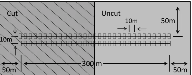
be an irregularly structured late-successional stands (> 120 years old) dominated by conifers (black spruce and balsam fir), and 3) roads had to be absent within a buffer (>50 m) around the transects in the cut stand. Each block included 2 or 3 sites separated by at least 100 m. Observations from the different sites were therefore largely independent because 1) 100 m corresponds approximately to the radius of a home-range (see results on the effects of logging on home range), and 2) individuals captured at a given site were rarely (2%) recaptured at another site. Within each site, we established a pair of 300-m parallel transects separated by 10 m (Fig. 3). One week after the beginning of our experiment, half of each site was clearcut (cut with protection of regeneration and soils, see Gauthier et al., 2008), which resulted in two adjactent habitat types: an old-growth forest stand (uncut) and a cut stand. The stands were cut so that the transects crossed the two habitats, and that each habitat was at least 200 × 100 m and shared a >100 m boundary with the adjacent habitat (Fig. 3).
Figure 3: Schematic view of one site corresponding to a pair of transects crossing the two habitats (cut and uncut stand) in boreal forest. The small rectangles correspond to live-trap locations.
300 m
10m
50m
Cut
Uncut
10m
50m
50m
19 SMALL MAMMAL TRAPPING
Small mammals were sampled along the two parallel 300-m transects crossing the two habitats (Fig. 2). Along each transect, live traps (7.7 8.8 23.0 cm; Sherman Traps, Tallahassee, Fla.) were placed every 10 m. We conducted three trapping sessions: 1) one week before, 2) less than a week after, and 3) one month after logging. Live traps were baited with apple (water and energy resource), organic cotton (nesting and isolation), and peanut butter (energy resource). They were inspected and re-set each morning for the three consecutive nights that comprised a trapping session. Captured red-backed voles (Myodes gapperi) were ear-tagged with a unique tag number (style 1005-1; National Band & Tag, Newport, Ky.), weighed, and measured before being released. We also determined sex and verified the reproductive status of females (i.e., lactating or pregnant). We classified each individual as an adult or juvenile according to its weight (18 g was considered juvenile) (Martell, 1983). For each site, we estimated the relative red-backed vole abundance as the minimum number known alive (MNA) per 100 trap-nights corrected for sprung traps (Beauvais and Buskirk, 1999). In addition, MNA was also calculated for adults, juveniles and reproductive females separately. Traps with non-target species were removed from the overall catching effort.
We used data from a past study (for details see Le Blanc et al., 2010) for the analysis of the abundance of red-backed voles in 1-year and 2-year old clearcuts. The experimental design was similar to ours, with the exception that a site consisted in a single 240-m transect crossing the two adjacent habitat types (i.e., 120 m in the cutover and 120 in the uncut stand). Individual sites (n = 16) were ≥100 m from one another. Small mammal trapping procedure was also similar to ours. We used the same calculation to estimate relative red-backed vole abundance, but we did not have the information to determine the age and the reproductive status of females.
20
TELEMETRY
We also equipped 12 male and 11 female red-backed voles with radiotransmitters (M1450 model, Advanced Telemetry Systems, Isanti, MN, USA). All collared females were either lactating, pregnant, or in estrus. To avoid an effect of collar weight (0.54 g) on behaviour, we only collared adults that were >20 g (White and Garrott, 1990). We monitored collared individuals between 7:00 and 16:00. Each vole was located by homing between 9 and 119 times (mean = 42.6, sd = 21.6) for 3 to 10 days (mean = 7, sd =1.76) before and after cutting. Relocations were at least 15 minutes apart. We categorized each individual as residing in either a clearcut (n=13) or an uncut stand (n=10) based on the majority of their locations during the radio-tracking.
HOME RANGE
We estimated home range size for each individual before and after logging using the 95% kernel (Worten 1989). We estimated the smoothing parameter (h) using the ad hoc method (Worton, 1989), and the median value of h was then applied to all individuals. The comparisons between home range estimates for different individuals are not affected by differences in the bandwidth, and any bias due to the bandwidth would affect all animals similarly (Davison, 2007). We also superimposed the post-harvest home range over the initial home range, and we calculated the percentage of overlap between the two. The percentage of overlap provided an index of site fidelity.
STATISTICAL ANALYSIS
To evaluate the short-term impact of logging on the abundance of red-backed voles, we used a generalized linear mixed model (GLMM) with a Gaussian distribution. We evaluated the variation of abundance through time (before vs less than a week and one month after cutting) as a function of the treatment (uncut vs cut). The GLMM took the general form:
21 Sites nested in blocks were considered a random effect in the model. We performed distinct analysis for four categories: all individual, adults, juveniles and reproductive females. We also compared the proportion (with logit transformation) of the adult population comprised of females (i.e., adult females / all adults) between cut and uncut stands for the three time intervals with the same GLMM structure (Eq. 1). For the clearcut of 1-2 year old, we also used a GLMM to evaluate the difference of abundance between the cut and uncut stand. The model was based on a hierarchically nested random effects design, whereby sites were nested in blocks which were nested in years.
We assessed the effects of logging on density-dependent habitat selection by red-backed voles using isodar theory (Morris, 1988). We determined the intercept and the slope of isodars with a model II simple linear regression using the major axis (MA) method with Gaussian distribution (Legendre and Legendre, 2012). The significance of the intercept and the slope was verified based on the 95% confidence intervals. To verify if our capture data provided empirical evidence of interference competition, we tested whether log-transformed abundances (log[x+1]) would provide a better fit than unlog-transformed densities (Morris, 1994). We used the R² to compare the fit of the two models. From the better model, isodars were then developed for different groups (all, adults and juveniles) and time relative to the treatment application (before, less than a week, and one month), for a total of 9 isodar models. We also built a 10th isodar for all individuals, 1-2 years after logging. Sites where no red-backed voles were captured in either the clearcut or the uncut stand of a given transect transect (Fig. 2) were removed from the analysis.
We tested the relationship between home range size and the number of locations to determine the minimal number of locations needed to estimate home range size (Appendix 2). We found that 20-25 locations were sufficient to determine home range size. We thus kept all the individuals which had at least 20 locations before and after logging (i.e., a total of 20 individuals, including 17 with ≥25 locations) (see Appendix 2). To evaluate the short-term impact of logging on home range size, we used an analysis of variance (ANOVA) for repeated measurements. We also used a t-test to compare the percentage of overlap between cut and uncut stands. All analyses were conducted in the statistical and data management software R (R Core Team 2013).
22
Results
Effects of logging on abundance
We captured 627 small mammals from 11 species during 9,559 trap-nights between June and October 2012 and 2013. Red-backed voles represented 70% of all captured individuals (442 different individuals). The remaining 30% of the total captures were composed of the following 10 species: Shrew (Sorex spp., 15%), red squirrel (Tamiasciurus hudsonicus, 5%), southern bog lemming (Synaptomys cooperi), deer mouse (Peromyscus maniculatus), northern short-tailed shrew (Blarina brevicauda), stoat (Mustela erminea), northern flying squirrel (Glaucomys sabrinus), eastern chipmunk (Tamias striatus), woodland jumping mouse, (Napaeozapus insignis), and meadow jumping mouse (Zapus hudsoniu).
Before the experiment, red-backed vole abundance was similar in the sites that were later logged than in the sites that remained uncut (t = 1.58, p = 0.12, n = 14). Their abundance remained similar between cut and uncut stands one week (t = -0.39, p = 0.70, n = 14) and one month after harvest (t = 1.62, p = 0.11, n = 14). Similar results were observed when the analysis was performed with adults only (Table 1). Although we also did not detect a change in juvenile abundance less than a week after harvest (t = 1.06, p = 0.30, n = 14), juvenile abundance was higher in cut than uncut stands one month after logging (t = 2.93, p < 0.01, n = 14). We captured 0.87 juvenile/100 trap-nights in uncut stands and 2.14 juveniles/100 trap-nights in clearcuts. Finally, there was a significant difference in the abundance of red-backed voles in 1-2 y clearcuts and in uncut stands (β ± S.E. = -3.67 ± 0.93, t = -3.95, p < 0.01, n = 16), with an average of 8.39 ind./100 trap-nights found and 4.73 ind./100 trap-nights in uncut stands.
The abundance of reproductive females decreased marginally more in cut than uncut stands (t = -1.92, p = 0.06, n = 14; Table 1). Indeed, while the abundance of reproductive females decreased from 0.76 ind./100 trap-nights before harvest to 0.31 ind./100 trap-nights one month after logging in the cut stand, the abundance in uncut stands increased from 0.33 reproductive female/100 trap nights to 0.41 ind./100 trap nights. According to the ratio of
23 females / adults, the proportion of females was similar in uncut stands than clearcuts before (t = 0.94, p = 0.37, n = 13) and one week after logging (t = 0.73, p = 0.48, n = 14). The proportion of females, however, became marginally higher in uncut than logged stands one month after harvest (β ± S.E. = -0.04 ± 0.02, t = -1.97, p = 0.07, n = 14).
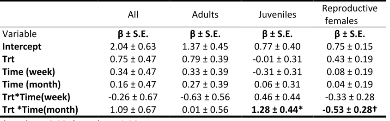
Table 1: Parameter estimates of GLMM models that assessed the short-term impact of logging on the abundance (individuals/100 trap-nights) of four categories of red-backed voles in the black spruce boreal forest of the Côte-Nord region of Québec (Canada) in 2012 and 2013. Treatment (Trt) refers to uncut vs cut stands, whereas Time contrasts before logging with one week and one month after logging.
Effects of logging on density-dependent habitat selection by red-backed voles
We were unable to detect evidence of interference competition based on the shape of isodars. First, both linear and log-log isodars had a similar fit before logging (untransformed: R² = 0.84 vs. log-transformed: R² = 0.81) and both types of isodar were non-significant one week after harvest. Second, one month after harvest, the linear isodar had a stronger fit (R² = 0.47) than the log-log isodar (R² = 0.34). We thus pursued the analysis based only on linear isodars.
When adults and juveniles were combined in the isodar analysis, the slope of the relationship before logging differed from 0 but not from 1 (β = 0.80, C.I. 95% = 0.59 – 1.07, n = 13, Appendix 1), indicating that the two parts of each stand can support the same
All Adults Juveniles Reproductive
females
Variable β ± S.E. β ± S.E. β ± S.E. β ± S.E.
Intercept 2.04 ± 0.63 1.37 ± 0.45 0.77 ± 0.40 0.75 ± 0.15 Trt 0.75 ± 0.47 0.79 ± 0.39 -0.01 ± 0.31 0.43 ± 0.19 Time (week) 0.34 ± 0.47 0.33 ± 0.39 -0.31 ± 0.31 0.08 ± 0.19 Time (month) 0.16 ± 0.47 0.27 ± 0.39 0.06 ± 0.31 0.04 ± 0.19 Trt*Time(week) -0.26 ± 0.67 -0.63 ± 0.56 0.46 ± 0.44 -0.33 ± 0.28 Trt *Time(month) 1.09 ± 0.67 0.01 ± 0.56 1.28 ± 0.44* -0.53 ± 0.28† *p-value < 0.05, † p-value = 0.06
24
abundance of red-backed voles regardless of vole density (Fig. 4a). Less than a week after logging, the relationship was not significant (β = 0.94, C.I. 95% = 0.09 – 6.70, n = 14) indicating the absence of density dependence in habitat selection between cut and uncut areas (Fig. 4b). One month later, the selection between cut and uncut stands was density dependent and the isodar’s slope was significantly lower than 1 (β = 0.52, C.I. 95% = 0.21 – 0.94, n = 14, Appendix 1), indicating that cut stands can support more individuals than uncut stands as competitor density increases (Fig. 4c). Finally, 1-2 years after logging, the slope of the relationship was again significantly higher than 0 but included 1 (β = 1.32, C.I. 95% = 0.81 – 2.35, n = 16, Appendix 1), indicating that cut and uncut stands can support the same abundance of red-backed voles, regardless of conspecific density (Fig. 4d).
25 Figure 4. Abundances of red-backed voles (juveniles and adults combined) between cut and old-growth forest, and the estimated isodar estimated: a) before, and b) less than a week, c) one month and d) one-two years after the logging. The dotted line corresponds to 1:1 line and the solid line is the regression line (displayed only if significant).
When the isodar was estimated based only adult red-backed voles, its intercept did not differ from 0 and its slope from 1 (β = 0.54, C.I. 95% = 0.20 – 1.03, n = 13, Appendix 1) (Fig. 5a) before logging. One week after logging, the isodar analysis did not detect any selection for either cutovers or uncut stands, and thus no density dependence in habitat selection as indicated by a slope non-significantly different from 0 (β = 0.74, C.I. 95% = -0.10 – 5.01, n = 14, Appendix 1) (Fig. 5b). One month after logging, however, the isodar’s
26
intercept did not differ from 0, and the slope was higher than 0 but not different from 1 (β = 0.64, C.I. 95% = 0.22 – 1.31, n = 14, Appendix 1) (Fig. 5c), indicating that adults were distributed similarly between the two stands.
Figure 5. Abundances of adult red-backed voles between cut and uncut old-growth forest, and the estimated isodar curves a) before b) less than a week and c) one month after the logging. Black dotted line in each figure corresponds to 1:1 line and the solid line corresponds to a regression (displayed only if significant).
The isodar did not reveal density dependence in the distribution of juvenile red-backed voles between cut and uncut sites, when the analysis was conducted on animal densities estimated either before logging (β = 0.53, C.I. 95% = -0.27 – 2.81, n = 9) or one week after the logging (β = 0.44, C.I. 95% = -0.42 – 2.75, n = 14, Appendix 1) (Fig. 6). One month later, however, the slope was significantly different from 0 (β = 0.38, C.I. 95% = 0.10 – 0.72 , n = 12, Appendix 1) and lower than 1, indicating that, as juvenile density increases, cut stands can support more juveniles than uncut stands (Fig. 6c).
27 Figure 6. Abundances of juvenile red-backed voles between cut and uncut old-growth forest, and the estimated isodars a) before, and b) less than a week and c) one month after the logging. The dotted line corresponds to 1:1 line and the solid line corresponds to a significant regression (displayed only if significant).
Effects of logging on home range
Home range sizes varied widely from 0.246 to 2.583 ha, with a mean size of 0.85 ± 0.43 ha (n = 40). We observed a decrease in home range size over time (F1,20 = 7.99, p = 0.01). The average reduction was slightly higher in cut than uncut stands (43% vs 30%), but the difference was non-significant (F1,20 = 0.20, p = 0.66). Finally, the percentage of overlap in the estimated home-range sizes did not differ before and after logging (F1,21 = 1.77, p = 0.12), and the overlap averaged 45.9% for voles located in clearcuts and 59.8% for those in uncut stands.
Discussion
Our study demonstrates rapid changes in the spatio-temporal dynamics of animal distribution and abundance following habitat disturbance. By combining ecological theory and field observations collected at three points in time, our study also reveals key biological processes driving the short-term dynamics of red-backed vole abundance exposed to timber harvest activities.
28
During the first week following logging, red-backed voles used cut stands as much as uncut ones, and there was no clear spatial structure in vole distribution. This could be attributed to a combination of factors such as increasing mortality in some clearcuts (the highest levels of abundance observed before logging were not reached soon after, Figs. 4a and 4b). Also, we observed a general reduction of movement as indicated by reduced home range size but continued site fidelity before/after. From its major impact on the density of mature stems and on the forest canopy, clearcutting reduces the protective cover and substantially increases the risk of predation for ground-dwelling species such as voles (Dussault et al., 1998). Also, silvicultural techniques, such as the cut with protection of regeneration and soils applied here, can leave relatively large amounts of woody debris and snags in the harvested sites (Gauthier et al., 2008, Swanson and Dryness, 1975). Further, such practices can leave protective cover for small animals, and provide potential food sources from fallen cones and xylophagous insects (Sullivan et al., 2011). Logging can thus impact both competition and predation, two density dependent processes. Yet the isodars did not detect any density dependence in habitat selection during this first week after harvest. Many ecological theories, including isodar theory, assume that animal distribution is at equilibrium. The lack of relationship between the abundance of voles in cut and uncut stands seem to indicate that logging has caused a short-term disruption in animal distribution dynamics, and the system might not be at equilibrium.
Density dependence in the local distribution of red-backed voles was back a month after logging. The abundance of voles in clearcuts then reflected the distribution in adjacent uncut forest. We outline a series of empirical trends indicating that, a month after logging, clearcuts may act as a population sink driven by interference competition. Indeed, the abundance of juvenile voles became higher in clearcuts than in adjacent uncut stands. Given that adults are generally dominant over juveniles (Boonstra and Krebs, 2012, Watts, 1970, Perrin, 1979), and that no change in abundance was detected for adults, the aggregation of juveniles in cuts supports the hypothesis that interference competition partly controls the spatial distribution of red-backed voles. Consistently, Powell (1972) observed that juvenile red-backed voles were three times more abundant in a recent blowdown than in undisturbed forests. He concluded that standing forest was the preferred habitat, but
29 adults drove juveniles into the less preferred, disturbed habitat through aggressive behaviour. Similarly, Campbell and Clark (1980) observed that juveniles outnumbered adults immediately after clearcuts. They showed an increase in juvenile voles two weeks to a month after logging, but not 9 to 12 months later. Female voles appeared to contribute strongly to the negative interactions. Relatively to clearcuts, uncut forests were occupied by a marginally (p = 0.07) larger proportion of adult females. Female voles, especially if they are breeding, are territorial and having mutually exclusive home range, whereas males have extensively overlapping home ranges (Boonstra and Krebs, 2012, Perrin, 1979).
Isodars did not provide any signal, however, that vole distribution might be ideal and despotic, because isodar models did not fit log-transformed abundances better than untransformed estimates. Detecting subtlety in the shape of regression lines often requires large datasets with values covering a broad range (e.g., Sarnelle and Wilson, 2008; Motulsky and Christopoulos, 2004), possibly exceeding what was available in our study. Moreover, interference competition appears to affect mostly a segment (i.e., juveniles) of the entire vole population. That being said, isodars still provided insights into the response of juveniles to competitor density. When conspecific abundance was low, juveniles were able to establish themselves equally in uncut than logged forests. It is only when the rate of captures of juveniles in uncut stands reached 1 individual per 100 traps-night that they gradually became more abundant in clearcuts (Fig. 6c).
Another finding supporting the notion that clearcuts would be of relatively poor quality habitat came from the distribution of reproductive females, as those females were less abundant in logged than uncut forest stands. Such negative effects would still not make clearcuts ecological traps. To be an ecological trap, individuals should overestimate the true fitness value of a given habitat (Robertson et al., 2013). Our results indicate, however, that the intensive use of clearcut by juveniles might have more to do with negative social interactions than a faulty assessment of habitat quality. Clearcuts would therefore be more closely associated to sink habitats. Although this hypothesis needs to be investigated further through studies of population growth in clearcut, it is consistent with our finding that 1-2 years after logging red-backed voles became less abundant in clearcuts than uncut stands. The hypothesis is also congruent with several studies showing that two years after logging