Procedia Engineering 163 ( 2016 ) 328 – 339
1877-7058 © 2016 The Authors. Published by Elsevier Ltd. This is an open access article under the CC BY-NC-ND license (http://creativecommons.org/licenses/by-nc-nd/4.0/).
Peer-review under responsibility of the organizing committee of IMR 25 doi: 10.1016/j.proeng.2016.11.067
ScienceDirect
25th International Meshing Roundtable
Efficient computation of the minimum of shape quality measures on
curvilinear finite elements
A. Johnen
a,b,∗, C. Geuzaine
a, T. Toulorge
c, J.-F. Remacle
baUniversity of Li`ege, Department of Electrical Engineering and Computer Science, Grande Traverse 10, 4000 Liege, Belgium bUniversit´e Catholique de Louvain, Institute of Mechanics, Materials and Civil Engineering (iMMC), Avenue Georges Lemaitre 4, 1348
Louvain-la-Neuve, Belgium
cCemef - Mines ParisTech, rue Claude Daunesse 1, 06904 Sophia-Antipolis, France
Abstract
We present a method for computing robust shape quality measures defined for any order of finite elements. All type of elements are considered, including pyramids. The measures are defined as the minimum of the pointwise quality of curved elements. The computation of the minimum, based on previous work presented by Johnen et al. (2013) [1,2], is very efficient. The key feature is to expand polynomial quantities into B´ezier bases which allows to compute sharp bounds on the minimum of the pointwise quality measures.
c
" 2016 The Authors. Published by Elsevier Ltd.
Peer-review under responsibility of the organizing committee of IMR 25.
Keywords: finite element method, finite element mesh, quality of curved elements, B´ezier basis
1. Introduction
With recent developments in the field of high-order finite element methods [3], such as discontinuous Galerkin [4] or spectral [5,6] methods, there is a renewed interest for high-order (curved) mesh generation. The classical finite element method, a.k.a. the h-version, uses linear elements to discretize the geometry and a refinement of the mesh is performed in order to increase the accuracy of the solution. It has been established that the p-version of the finite element, for which the order of the functions is increased in order to improve the accuracy, may provide better conver-gence [7]. Eventually, “super-converconver-gence” can be obtained by a mix of the two approaches [8]. There has thus been a frenzy in the 1980s to develop such methods, but developers encountered several difficulties which hampered their momentum [9]... and consequently most of the current industrial-grade and commercial finite element packages are still based on at most second-order meshes. One reason is that during the process of generating a high-order curvilin-ear mesh, invalid (tangled) elements are often created, and untangling those is not a trivial task. Recent methods have improved the robustness of the untangling procedure through optimization, albeit at a high computational cost [10].
∗Corresponding author.
E-mail address: amaury.johnen@uclouvain.be
© 2016 The Authors. Published by Elsevier Ltd. This is an open access article under the CC BY-NC-ND license (http://creativecommons.org/licenses/by-nc-nd/4.0/).
For this reason, the tendency is to apply the technique only on small groups of elements in the neighborhood of the invalid elements to untangle. It is therefore crucial to be able to detect invalid and poor-quality curvilinear elements.
A finite element is defined by the position of its nodes through a mapping between a reference element and itself. Its validity can thus be assessed by verifying the positivity of the determinant of the Jacobian of this mapping. It was thought for years that the only way to determine with certainty the validity of non-trivial elements would be by computing the Jacobian determinant at an infinite number of points [11,12]. Recent developments based on B´ezier interpolation showed that it is nothing of the sort. A first step has been taken in [13] where it is shown that it is possible to compute bounds on the Jacobian determinant of second order tetrahedra; those bounds are however not sharp. References [1,2] provided a complete solution by developing an adaptive technique for efficiently computing the minimum and the maximum of the Jacobian determinant of any type and any order of elements, up to any prescribed tolerance. This method subsequently allows to guarantee the validity of any element.
Validity is one aspect that influences the accuracy of solution. Another aspect is the quality of the finite elements. A distinction can be made between geometric quality measures and Jacobian-based quality measures. Geometric quality measures have been used since the very early days of finite element modeling and are constructed from geometric characteristics such as the area/volume of the element, the length of the edges or the radii of the inscribed and circumscribed circles/spheres [14,15]. These geometric quality measures are however not easily generalizable to curved elements—see e.g. [13] for the extension to quadratic tetrahedra. Jacobian-based measures are a more natural fit, since the Jacobian matrix is defined for every order and every type of element. A framework that allows the construction, classification, and evaluation of such measures defined on linear elements has been proposed in [16,17]. It is important to understand that Jacobian-based measures are essentially pointwise (within the element). For the linear triangles and tetrahedra, this is not a problem since the Jacobian matrix is constant. For other elements, an element-wise measure has to be extracted from the pointwise measure. In the two references above, it is proposed to compute the measure at the corners of linear quadrangles and hexahedra and to take the minimum or the harmonic or geometric average. Similarly, for quadratic triangles, the element-wise measure can be computed as the minimum, maximum or the pthpower-mean of the pointwise measure sampled at the six nodes of the elements, although it is shown that in some situations this constitutes a poor approximation of the true minimum, maximum or pth power-mean [12].
Recent works have focused on defining a quality measure for curved simplicial finite elements of any order [18, 19]. The general approach is to consider the inverse of a Jacobian-based quality measure as proposed in [16], which constitutes a pointwise distortion measure. The L2-norm is computed in order to have an element-wise measure and the quality of the element is defined as the inverse of this element-wise distortion. The chosen distortion is such that it goes to infinity for degenerate (invalid) elements which implies that the corresponding quality vanishes. However, since the distortion measure is not a polynomial (it is at best a rational function), no exact computation of the measure is proposed and degenerate elements cannot robustly be detected by this method. Although developed for simplicial elements, this technique can be extended to non-simplicial elements, as shown in [20].
In this paper, we propose to extend the method that efficiently computes the extrema of the Jacobian determinant as proposed in [1,2] to Jacobian-based quality measures. Instead of computing the element-wise quality measure by simply taking a norm, we aim at finding the actual bounds of the pointwise measure.
The paper is organized as follows. In Section 2, we begin by recalling the Jacobian matrix of the different mappings before presenting the shape quality measures considered in this paper. In Section 3, we present the B´ezier expansion, we recall the algorithm for computing bounds on the validity of the elements and we give some properties of B´ezier expansions that are useful for computing bounds on the quality measures. In Sections 4, we explain how to compute those bounds. Finally, results are presented in Section 5 and we conclude in Section 6.
2. Definition of quality measures for curvilinear finite elements
Let us consider a mesh of order n, which consists of a set of curved physical elements that can either be triangles and/or quadrangles if the mesh has 2 dimensions or tetrahedra, hexahedra, prisms and/or pyramids if the mesh has 3 dimensions. 3D meshes are always defined in a 3 dimensional space. However, 2D meshes can either live in the xy-plane or be embedded inside a (in general non-planar) 3D surface. Let dmand dsdenote respectively the dimension of the mesh and the dimension of the physical space in which the mesh is embedded. Each physical element is defined
geometrically through a set of points of the physical space, called nodes,nk∈ Rds,k = 1, . . . , N and a set of Lagrange shape functions Ln
k(ξ) : Ωref⊂ Rdm→ R, k = 1, . . . , N. These functions are polynomial and allow to map a reference unit element, whose domain of definition is Ωref, onto the physical one (see Fig. 1):
x(ξ) = N ! k=1 Ln k(ξ)nk. (1)
Among the considered elements, pyramids are quite particular. Those elements which consist of a quadrangular base and four triangular faces have 4 edges that are incident to the summit node and cannot be defined by a polynomial mapping. Many different solutions have been proposed in the literature and among them, we consider the definition proposed in [21] that has optimal error estimates in H1-norm. Instead of polynomials, the mapping is defined by rational functions. Nevertheless, it has been shown that computing bounds on the Jacobian determinant of pyramids using the technique described in [1] is done as if it was defined by polynomials [2]. For simplicity, we will consider that all the elements have polynomial shape functions.
ξ1 ξ2 Reference ξ1 ξ2 Ideal x y Physical JR W JI
Fig. 1. We consider three mappings, each of them is characterized by a Jacobian matrix: (1)JRfor the mapping between the reference and the
physical element, (2)W for the mapping between the reference element and the ideal element and (3) JIfor the mapping between the ideal and the
physical element.
The Jacobian matrix of the mapping between the reference and the physical element, denoted byJR, is in general not constant over the element: JR: Ωref→ Rds×dm: ξ '→ JR(ξ). It is by definition the matrix of the first-order partial derivatives, i.e. (JR)i j = ∂x∂ξij, which are polynomial functions. JRcontains all the information of the transformation
of the reference element into the physical element and can naturally be used to construct quality measures. However, as explained in [16], it may be necessary to compare the physical element to an ideal element which defines the ideal shape. This ideal element is usually the equilateral triangle or the square for 2D elements. We note the Jacobian matrix of the mapping between the ideal and the physical element JI. This matrix can be computed by the product JI=JRW−1, whereW is of dimesion dm×dmand is the Jacobian matrix between the reference and the ideal element. In this paper, we make the assumption thatW is a constant matrix, therefore that the mapping between the reference and the ideal element is affine. We thus only consider ideal elements that are linear, have planar faces and (when appropriate) have parallel opposite sides. For instance, the ideal quadrangle can be a parallelogram but not a trapeze. This implies that the elements ofJIremain polynomials, which is a necessary condition for computing the bounds the way it is described in this paper.
In the following subsections, we first define two pointwise shape quality measures and we define the element-size measure. Note that we consider only valid elements. The two considered measures are equal to zero for invalid elements.
2.1. The isotropy measure
Let us consider the following quantity defined on any given element E [16,20,22,23]: ηpw(E, ξ) =dm|JI|
2 dm
||JI||2F
where |·| is the determinant of a square matrix and ||·||F is the Frobenius norm of a matrix, i.e. ||·||2F is the sum of the squares of the matrix elements. It follows from Proposition 8.7 and 9.5 of [16] that this quantity is equivalent to measure the distance ofJIto the set of singular matrices (matrices whose determinant is zero) and thus, ηpwmeasures the pointwise distance to a locally degenerate element. It constitutes a shape quality measure (Proposition 9.3 of the same paper) which takes the maximum value of 1 when the element is locally of the same shape than the ideal element. We call this measure isotropy since the more it goes to 0, the more locally anisotropic is the element, which is strongly related to the conditioning of stiffness matrices [15]. Note that a more accurate measure for the conditioning of stiffness matrices has been considered in [24] (see Section 3 and Appendix E). The algorithm to compute that measure is however very complex and leads to computation times that are about 10 times higher than the measure we consider in this paper.
2.2. The scaled Jacobian measure
The scaled Jacobian is extensively used for measuring the quality of quadrangles and hexahedra [25–33]. Letvjbe the jth column of the matrixJI. The scaled Jacobian is defined as
σpw(E, ξ) ="|JI| j######vj######2
.
This measure is closely related to the interpolation error of the finite element solution [15] and takes its value between 0 and 1, with 1 being for the best shape and 0 the worst. Note that another
2.3. Definition of an element-wise measure
In order to define an element-wise measure, we take the minimum of the pointwise measure: η(E) = min
ξ∈ Ωref
ηpw(E, ξ), σ(E) = min ξ∈ Ωref
σpw(E, ξ).
The rationale behind this is that it is certainly possible to bound the error of the finite element solution with this measure the same way we can bound the error by looking at the worst element of straight-sided meshes.
3. B´ezier expansion
Polynomial quantities can be expanded into a so-called B´ezier basis in order to make use of the well-known B´ezier expansion properties. We introduce in this section all the concepts concerning the B´ezier expansion that will be useful in this paper. Note that we use the multi-index notation for whichi = (i1, . . . ,idm) is an ordered tuple of dmindices.
Let Bν
i(ξ) : Ωref ⊂ Rdm → R, i ∈ Iνdenotes a B´ezier function of order ν where Iνis the index set of the B´ezier functions. Both Bν
i and Iν depend on the type of the element. The analytical expression of B´ezier functions for linear, triangular, quadrangular, tetrahedral, hexahedral and prismatic elements are given in [1] and the expression for pyramidal elements is given in [2]. The set {Bν
i}i∈Iν defines the B´ezier basis of the polynomial space of order
ν. Let fidenote the coefficients of the expansion, also known as the control values. For any polynomial function f : Ωref⊂ Rdm→ R of order at most ν, one can compute the control values such that we have the following equality:
f (ξ) = ! i ∈ Iν
fiBνi(ξ), where the right member is the B´ezier expansion of the function f .
The B´ezier functions are positive and sum up to one which implies the well-known convex hull property. In our case, the convex hull property says that f is bounded by the extrema of the control values, i.e. minifi≤ f (ξ) ≤ maxifi. In addition to that, there are control values that are actual values of the expanded function. Those control values are
“located” on the corners of the element1and we refer to their index set by Iν
c . As a consequence, the control values allow to bound the two extrema of the function from below and above. For example, for the minimum we have: minifi≤ fmin≤ mini∈Iν
c fi.
Those bounds, computed from the B´ezier expansion, are not necessarily sharp. However, they can be sharpened by subdividing, i.e. by expanding the same function defined on a smaller domain, called a subdomain. The smaller the subdomain, the sharper the bounds. This subdivision can be implemented in a recursive and adaptive manner which makes the method very efficient [1]. The algorithm for computing sharp bounds on polynomial functions consists of four steps:
1. Sampling of the function on a given set of points.
2. Transformation of those values into B´ezier coefficients (by a matrix-vector product). 3. Computation of the bounds. If the sharpness is reached, return the bounds.
4. Subdivision (through a matrix-vector product). For each subdomain, go to step 3. Gather the “subbounds” and compute and return the global bounds.
We propose to adapt this algorithm to the computation of bounds of ηpwand σpw. As it will be seen later, only the third step has to be adapted. Additional properties of the B´ezier expansion will be needed and are given in the following. Observation 1. Any B´ezier function (even pyramidal) is of the canonical form Bν
i(ξ) = ανimνi(ξ), where the coefficient αν
i is a product of binomial coefficients and mνi is the elementary function. As an example, let us consider the triangular B´ezier functions:
Bν i1,i2(ξ, η) = $ν i1 %$ν− i 1 i2 % ξi1ηi2(1 − ξ − η)ν−i1−i2. Its coefficient is αν i1,i2= &ν i1 '&ν−i1 i2 '
and its elementary function is mν
i1,i2(ξ) = ξ
i1ηi2(1 − ξ − η)ν−i1−i2.
Observation 2. The product of two elementary functions mν
i and mµjis an elementary function equal to mν+µi+ j. Example: mν i1,i2m µ j1,j2= ξ i1+j1ηi2+j2(1 − ξ − η)ν+µ−(i1+j1)−(i2+j2)=mν+µ i1+j1,i2+j2.
Corollary 3. The product of two B´ezier functions of order ν and µ is a B´ezier function of order ν+µ with an adjustment coefficient: Bν iBµj= αν iαµj αν+µi+ j B ν+µ i+ j.
Observation 4. Let f and g be two polynomial functions of respective order ν and µ and let fi, i ∈ Iνand gj, j ∈ Iµ be their respective control values. The product of f and g is a polynomial function of order ν + µ whose control values hkare equal to:
hk= ! i∈Iν j∈Iµ i+ j=k figj αν iαµj αν+µk , ∀k ∈ I ν+µ.
Proof. Using the definition of the B´ezier expansion and Corollary 3, we have the following equalities: h = f g =! i∈Iν j∈Iµ figj αν iαµj αν+µi+ j B ν+µ i+ j = ! k∈Iν+µ ! i∈Iν j∈Iµ i+ j=k figj αν iαµj αν+µk B ν+µ k . 1 Let ξ
cbe the reference coordinates of one of the corners of the element. For any B´ezier basis, there exists an indexj such that Bνj(ξc) = 1 and
Bν
Proposition 5. Relaxation: Let f and g be two polynomial functions of order ν and let fi and gi, i ∈ Iνbe their respective control values. In order that f(ξ) ≤ g(ξ), ∀ξ ∈ Ωref, it is sufficient that fi≤ gi, ∀i ∈ Iν.
Proof. Since every B´ezier function is positive on the reference domain,
fi≤ gi ⇒ fiBνi(ξ) ≤ giBνi(ξ) ∀ξ ∈ Ωref,∀i ∈ Iν.
The last proposition can be used to compute bounds on more complex functions. The following sections explain how to do it for rational functions and functions that are similar to a quadratic mean, i.e. that are written(f2
1 +f22+ . . . where the fkare polynomial functions.
3.1. Computing bounds on rational functions
It is possible to compute bounds on rational functions whose denominator is known to be strictly positive or strictly negative. There are four cases depending on the sign of the denominator and if a lower or an upper bound is required. In the following, we detail the method for computing a lower bound in the case of a strictly positive denominator. The adaptation for other cases is straightforward.
Let gf (g > 0) be the rational function, with f and g two polynomial functions and let rmdenote the lower bound of this rational function we want to compute. Since g is strictly positive, the lower bound has to satisfy rmg ≤ f . Let fiand gi,i ∈ Iνbe the control values of their respective B´ezier expansion. Taking advantage of the relaxation (Proposition 5), we can solve the following problem:
max rm
s.t. rmgi≤ fi ∀i ∈ Iν.
This is an optimization problem with only one variable which is therefore easily solved. Note that the coefficients gican take a negative value even if g is strictly positive. The inequalities represent upper or lower bounds for rmin function of the sign of gi. Two situations may happen at the end: The global lower bound can be larger than the global upper bound, in which case the problem is unsolvable, otherwise rmis equal to the upper bound. Special cases happen when gi=0. In the one hand, if fi≥ 0, the inequality is satisfied whatever the value of rm. In the other hand, if fi<0, the inequality cannot be satisfied and the problem is unsolvable.
3.2. Computing bounds with quadratic mean-like functions
When a square root is present in an expression we want to bound, it may be possible to square the expression in order to obtain only polynomials. However, it is possible to construct a function that bound from the above quadratic mean-like functions, as proved by the following lemma:
Proposition 6. Let f and g be two polynomial functions of order ν and let fiand gibe their control values. Let H be the function whose control values are Hi=
( f2
i +g2i. Then, we have )
f (ξ)2+g(ξ)2≤ H(ξ) ∀ξ. Proof. Since the two members of the inequality are positive, we can square the expression:
! i fiBνi(ξ) 2 + ! i giBνi(ξ) 2 ≤ ! i ( f2 i +g2i Bνi(ξ) 2 ⇔! i, j & fifj+gigj'Bνi(ξ)Bνj(ξ) ≤ ! i, j ( f2 i fj2+fi2g2j+g2i f2j +g2ig2jBνi(ξ)Bνj(ξ). By the relaxation of Proposition 5, it is sufficient to prove the following inequalities:
fifj+gigj ≤ (
f2
The right-hand member is positive. This implies that the relation is satisfied if the relation hold when the members are squared. We obtain:
2 fifjgigj ≤ fi2g2j+g2i fj2 ∀i, j ⇔ 0 ≤&figj− gifj'2 ∀i, j, which is true.
Note that this lemma can be generalized to any function of the form (f2
1 + f22+f32+ . . .where the fk are poly-nomial functions. This result is useful in order to avoid to compute more coefficients as it is shown in the following section.
4. Computing bounds on the quality measures
Computing bounds on the considered quality measures relies on the fact that the steps 1, 2 and 4 of the algorithm described in Section 3 works for any polynomial function. We can thus identify polynomial components of a given measure and directly apply steps 1,2 and 4 to those components. Only the computation of the bounds in replacement of the 3rd step has to be particularized.
The two measures can be computed from the same polynomial components. Let ai, j, i, j = 1, . . . , dmdenote the elements of the Jacobian matrix JI. They are polynomial functions and can be expanded into the B´ezier basis of the mapping (1), i.e. into {Bn
i}i∈In. From this data alone (i.e. from the B´ezier coefficients of the ai, j), it is possible to
compute the Jacobian determinant, the Frobenius norm ofJIand the 2-norm of the columns ofJI, which is sufficient to compute the two measures. However, computing the Jacobian determinant from the ai, jis costly and we prefer to directly expand |JI|. Contrary to [1,2], the B´ezier basis in which it is expanded cannot be reduced for certain types of elements, it has to be {B2n
i }i∈I2nfor 2D elements and {B3ni }i∈I3nfor 3D elements.
4.1. The isotropy measure
In 2D, the isotropy measure is 2 |JI| / ||JI||2F, where ||JI||2F =0i, ja2i, j. The B´ezier coefficients of the numerator are available since it is the Jacobian determinant. The denominator is also a polynomial function and the lower bound of the measure can be computed by the rational function technique provided that the denominator is expanded into the same B´ezier basis than the numerator (Section 3.1). To do so, the expansion of the terms a2
i, jis computed thanks to Proposition 4 and then the B´ezier coefficients of the denominator are computed by linearity.
In 3D, the measure is 3 |JI|23/||JI||2
F. In order to have a polynomial function at the numerator, the expression can be raised to the power of 3
2while still allowing us to compute a bound. Indeed, since the exponentiation is a monotonic operation and the measure is positive, whatever the bound r of η3/2pw we compute, we will have that r23 is a bound of
ηpw. The denominator of the new expression is:
||JI||3F = 1 2 3!3 i, j=1 a2 i, j 3 .
Due to the presence of the square root and since we are interested by a lower bound of the measure, we compute an upper bounding function of ||JI||F by the technique described in Section 3.2. Afterwards, we apply Proposition 4 in order to obtain an expansion of the denominator into the same B´ezier basis than the numerator. The rational function technique can then be applied in order to compute the lower bound of the measure.
Let us recall that in 2D and 3D, an upper bound of the minimum of the measure is computed from the “corner” coefficients as explained in Section 3.
4.2. The scaled Jacobian
The technique for computing a lower bound of the scaled Jacobian for quadrangles or hexahedra is the same. As for the other measure, we have to expand the denominator into the same B´ezier basis than the numerator. The terms of the denominator are######vj######2= (0ia2i, j. Since we are interested by a lower bound of the measure, we compute upper bounding functions Vjof######vj######2by the technique described in Section 3.2. The expansion of the denominator is then obtained by applying Proposition 4 on "jVj. Finally, the rational function technique gives the lower bound. 5. Results
The algorithm described in this paper is implemented in Gmsh [34] and can be tested through the plugin
AnalyseCurvedMesh. We begin this section by testing two linear hexahedra. Then we test an academic hexahedral mesh with high differences in aspect ratio. After, we test a more realistic mesh composed of curved tetrahedra. All the tests has been conducted on a Macbook Pro Retina, Mid 2012 @ 2.3GHz.
5.1. Single hexahedron test
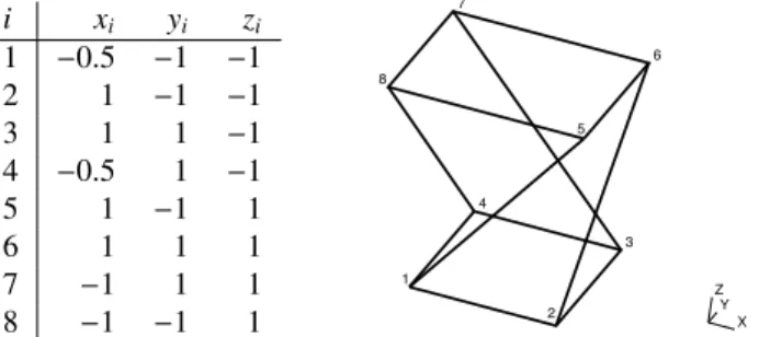
Let us consider the case of a single hexahedron for which the nodes location is given in Table 2 of reference [11]. This hexahedron has positive Jacobian determinant on all the edges but is invalid. Traditional methods would compute a non-zero quality. Our algorithm computes the correct value of η = σ = 0. Now let us consider a more interesting case of a twisted hexahedron whose nodes location is given in Figure 2. This hexahedron is
i xi yi zi 1 −0.5 −1 −1 2 1 −1 −1 3 1 1 −1 4 −0.5 1 −1 5 1 −1 1 6 1 1 1 7 −1 1 1 8 −1 −1 1 1 2 3 4 5 6 7 8 Z X Y
Fig. 2.Twisted hex: Location and ordering of the nodes. Note that the convention for node order the one used in the Gmsh software.
valid and the measures computed at a tolerance of 1e−7 are in the range σ ∈ [0.6891687332,0.6891687876] and
η∈ [0.5799706988,0.5799707886]. The minimum of σpwat the corners of the element is 0.6963, which is an error
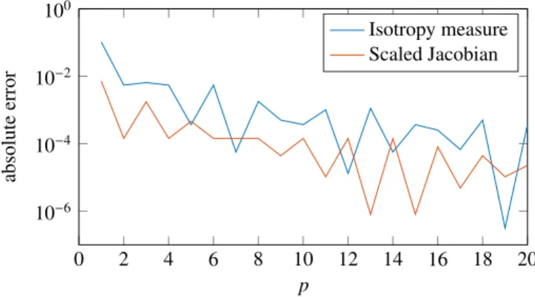
of 0.0071, while the minimum ηpwat the corners of the element is 0.6832, i.e. a substantial error of 0.1032. In order to compare with the basic method which consists in sampling the pointwise measure at a large number of points, let us consider the nodes of an hexahedron of order p. We sample the measures at the location of those nodes and compute the absolute error. As shown in Figure 3, the error decreases slowly. With p = 20, which corresponds to 9, 261 sampling points, the error is still 3.68e−4for the isotropy measure and 2.27e−5for the scaled Jacobian. 5.2. Academic hexahedral mesh
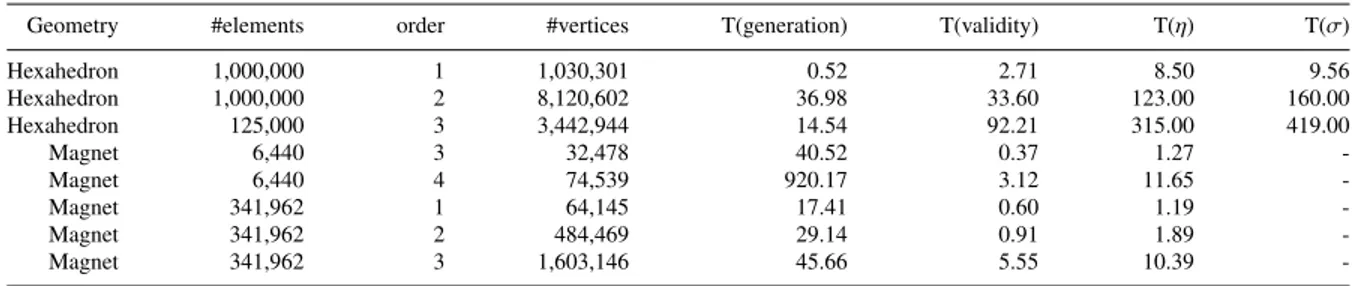
We now test the measures on a series of academic meshes composed of structured hexahedra. The meshes are generated with a mapping technique and presents high differences in sizes and aspect ratio, see Figure 4. Three meshes are generated: a linear and a second-order mesh of 1, 000, 000 hexahedra and a third-order mesh of 125, 000 hexahedra. For each mesh, the generation time and the time to compute the two measures are reported at Table 1. We also report in the same table the time to compute the validity of the different meshes, which corresponds to the time to compute the minimum and the maximum of the Jacobian determinant [1].
0 2 4 6 8 10 12 14 16 18 20 10−6 10−4 10−2 100 p absolute error Isotropy measure Scaled Jacobian
Fig. 3.Twisted hex: Absolute error of the sampling of ηpwand σpwat the nodes of an hexahedron of order p.
Fig. 4.Hex mesh: Coarse version (with 8,000 hexahedra) of the academic 1,000,000 and 125,000 hexahedra test cases.
It is important to highlight that the mapping technique is characterized by a particularly fast execution time in comparison to the generation of other kind of meshes. Even though, the computation of one quality measure in those three tests is at most 29 times slower than the generation (for computing the scaled Jacobian on the third-order mesh). Compared to validity computation, the computation of one quality is at most 4.8 times slower (for computing the scaled Jacobian on the second-order mesh). The worst and best elements according to the scaled Jacobian are shown in Figure 5. As expected, the best elements have nearly the shape of a rectangular parallelepiped while the worst have large angles.
5.3. Realistic curved tetrahedral mesh
Finally, we experiment the isotropy measure on a more realistic geometry that is meshed with tetrahedra. A coarse and a fine mesh are generated and optimized using the method presented in [10], see Figure 6. Computation times are presented in Table 1. Note that, proportionally to the number of elements, the geometrical optimization takes more times when applied to the coarse mesh than when applied to the fine mesh, which is because of the elongated/flat elements present inside the mountain box of the coarse mesh that are harder to optimize. This explains the particularly long generation time for the coarse mesh of order 4. A similar tendency appears with the computation of the validity and the isotropy measure which takes more time on the coarse mesh than the fine mesh, proportionally to the number of elements. This is the consequence of a greater proportion of straight-sided elements and the presence of curved
Fig. 5.Hex mesh: Worst (left) and best (right) quality elements of the coarse mesh.
Fig. 6.Curved tetrahedral mesh: The geometry models a sensor for a steel cable. The geometry is composed of 4 coils (in orange), the cable (in blue) and the mounting box (in red). In purple and in green are respectively the interior and the exterior meshes of the voids. Left: coarse mesh. Right: fine mesh.
elements that are less distorted in the fine mesh. On the average, the number of subdivisions per element needed to attain the desired tolerance is 0.0414 for the fine mesh of order 3 and 1.7888 for the coarse mesh of order 3. The maximum number of subdivision on an element is 5 and 19 for the fine and coarse mesh of order 3 respectively. Contrary the hexahedral mesh, the computation of the measure for this case is smaller than the generation time. The worst elements of the coarse mesh are shown in Figure 7.
6. Conclusion
A method for computing the minimum of pointwise shape quality measures defined for any order and any type of common finite elements (including pyramids) has been presented. Two measures has been considered. The first one, the isotropy measure, gives the distance of the element to the degeneracy and is related to the conditioning of the stiffness matrix. The second one, the scaled Jacobian, is defined for quadrangles and hexahedra and is related to the bound on the gradient of the error of the finite element solution. The computation is efficient and numerical
Table 1. Computation times of each test performed on the hexahedral and the tetrahedral mesh. Times are given in seconds. The generation time comprises the creation of 1D, 2D and 3D elements, the topological optimization of tetrahedral meshes (using Netgen [35]) and the geometrical optimization of high-order meshes (using [10]). T(η) and T(σ) are the times to compute the measures described in this paper while T(validity) is the time to compute [1].
Geometry #elements order #vertices T(generation) T(validity) T(η) T(σ)
Hexahedron 1,000,000 1 1,030,301 0.52 2.71 8.50 9.56 Hexahedron 1,000,000 2 8,120,602 36.98 33.60 123.00 160.00 Hexahedron 125,000 3 3,442,944 14.54 92.21 315.00 419.00 Magnet 6,440 3 32,478 40.52 0.37 1.27 -Magnet 6,440 4 74,539 920.17 3.12 11.65 -Magnet 341,962 1 64,145 17.41 0.60 1.19 -Magnet 341,962 2 484,469 29.14 0.91 1.89 -Magnet 341,962 3 1,603,146 45.66 5.55 10.39
-Fig. 7.Curved tetrahedral mesh: Worst elements of the coarse mesh. Those elements are unsurprisingly located inside the mounting box.
experiments show that for realistic third-order tetrahedral meshes the computation time of the quality measure is of the same order as the mesh generation time.
While the first measure works well for isotropic meshes but not for anisotropic meshes, the second measure can be used when curved high aspect ratio quadrangles and hexahedra are needed, as for example in boundary layer meshes with high curvature. A possible extension is the generalization of the scaled Jacobian to the other type of elements. Another extension would be to consider the adaptation of the isotropy measure for anisotropic meshes. Moreover those shape quality measures could give a robust base for the optimization of curvilinear meshes.
Acknowledgements
This research project was funded in part by the Walloon Region under WIST 3 grant 1017074 (DOMHEX) and by TILDA project. The TILDA (Towards Industrial LES/DNS in Aeronautics - Paving the Way for Future Accurate CFD) project has received funding from the European Unions Horizon 2020 research and innovation programm under grant agreement No 635962. The project is a collaboration between NUMECA, DLR, ONERA, DASSAULT, SAFRAN, CERFACS, CENAERO, UCL, UNIBG, ICL and TsAGI.
References
[1] A. Johnen, J.-F. Remacle, C. Geuzaine, Geometrical validity of curvilinear finite elements, Journal of Computational Physics 233 (2013) 359–372.
[2] A. Johnen, C. Geuzaine, Geometrical validity of curvilinear pyramidal finite elements, Journal of Computational Physics 299 (2015) 124–129. [3] Z. J. Wang, K. Fidkowski, R. Abgrall, F. Bassi, D. Caraeni, A. Cary, H. Deconinck, R. Hartmann, K. Hillewaert, H. T. Huynh, et al., High-order
CFD methods: current status and perspective, International Journal for Numerical Methods in Fluids 72 (2013) 811–845.
[4] R. M. Kirby, S. J. Sherwin, B. Cockburn, To CG or to HDG: a comparative study, Journal of Scientific Computing 51 (2012) 183–212. [5] P. E. J. Vos, S. J. Sherwin, R. M. Kirby, From h to p efficiently: Implementing finite and spectral/hp element methods to achieve optimal
performance for low-and high-order discretisations, Journal of Computational Physics 229 (2010) 5161–5181.
[6] G. Karniadakis, S. Sherwin, Spectral/hp element methods for computational fluid dynamics, Oxford University Press, 2013.
[7] I. Babuˇska, B. A. Szabo, I. N. Katz, The p-version of the finite element method, SIAM Journal on Numerical Analysis 18 (1981) 515–545. [8] I. Babuˇska, B. Q. Guo, The h-p version of the finite element method for domains with curved boundaries, SIAM Journal on Numerical Analysis
25 (1988) 837–861.
[9] R. H. MacNeal, Finite Elements, CRC Press, 1993.
[10] T. Toulorge, C. Geuzaine, J.-F. Remacle, J. Lambrechts, Robust untangling of curvilinear meshes, Journal of Computational Physics 254 (2013) 8–26.
[11] P. M. Knupp, On the invertibility of the isoparametric map, Computer Methods in Applied Mechanics and Engineering 78 (1990) 313–329. [12] P. Knupp, Label-invariant mesh quality metrics, in: Proceedings of the 18th International Meshing Roundtable, Springer, 2009, pp. 139–155. [13] P. L. George, H. Borouchaki, Construction of tetrahedral meshes of degree two, International Journal for Numerical Methods in Engineering
90 (2012) 1156–1182.
[14] D. A. Field, Qualitative measures for initial meshes, International Journal for Numerical Methods in Engineering 47 (2000) 887–906. [15] J. R. Shewchuk, What is a good linear finite element? interpolation, conditioning, anisotropy, and quality measures (preprint), 2002. Preprint. [16] P. M. Knupp, Algebraic mesh quality metrics, SIAM Journal on Scientific Computing 23 (2001) 193–218.
[17] P. M. Knupp, Algebraic mesh quality metrics for unstructured initial meshes, Finite Elements in Analysis and Design 39 (2003) 217–241. [18] X. Roca, A. Gargallo-Peir´o, J. Sarrate, Defining quality measures for high-order planar triangles and curved mesh generation, in: Proceedings
of the 20th International Meshing Roundtable, Springer, 2012, pp. 365–383.
[19] A. Gargallo-Peir´o, X. Roca, J. Peraire, J. Sarrate, Distortion and quality measures for validating and generating high-order tetrahedral meshes, Engineering with Computers (2014) 1–15.
[20] A. Gargallo Peir´o, Validation and generation of curved meshes for high-order unstructured methods, Ph.D. thesis, Universitat Polit`ecnica de Catalunya, 2014.
[21] M. Bergot, G. Cohen, M. Durufl´e, Higher-order finite elements for hybrid meshes using new nodal pyramidal elements, Journal of Scientific Computing 42 (2010) 345–381.
[22] A. Liu, B. Joe, On the shape of tetrahedra from bisection, Mathematics of Computation 63 (1994) 141–154. [23] A. Liu, B. Joe, Relationship between tetrahedron shape measures, BIT Numerical Mathematics 34 (1994) 268–287.
[24] A. Johnen, Indirect quadrangular mesh generation and validation of curved finite elements, Ph.D. thesis, Universit´e de Li`ege, 2016.
[25] P. M. Knupp, Achieving finite element mesh quality via optimization of the Jacobian matrix norm and associated quantities. part I—A framework for surface mesh optimization, International Journal for Numerical Methods in Engineering 48 (2000) 401–420.
[26] P. M. Knupp, Achieving finite element mesh quality via optimization of the Jacobian matrix norm and associated quantities. part II—A framework for volume mesh optimization and the condition number of the jacobian matrix, International Journal for Numerical Methods in Engineering 48 (2000) 1165–1185.
[27] S. Yamakawa, K. Shimada, Fully-automated hex-dominant mesh generation with directionality control via packing rectangular solid cells, International Journal for Numerical Methods in Engineering 57 (2003) 2099–2129.
[28] Y. Zhang, C. Bajaj, Adaptive and quality quadrilateral/hexahedral meshing from volumetric data, Computer Methods in Applied Mechanics and Engineering 195 (2006) 942–960.
[29] Y. Ito, A. M. Shih, B. K. Soni, Octree-based reasonable-quality hexahedral mesh generation using a new set of refinement templates, Interna-tional Journal for Numerical Methods in Engineering 77 (2009) 1809–1833.
[30] M. L. Staten, R. A. Kerr, S. J. Owen, T. D. Blacker, M. Stupazzini, K. Shimada, Unconstrained plastering—Hexahedral mesh generation via advancing-front geometry decomposition, International Journal for Numerical Methods in Engineering 81 (2010) 135–171.
[31] N. Kowalski, F. Ledoux, P. Frey, Automatic domain partitioning for quadrilateral meshing with line constraints, Engineering with Computers (2014) 1–17.
[32] J. H.-C. Lu, I. Song, W. R. Quadros, K. Shimada, Geometric reasoning in sketch-based volumetric decomposition framework for hexahedral meshing, Engineering with Computers 30 (2014) 237–252.
[33] T. C. Baudouin, J.-F. Remacle, E. Marchandise, F. Henrotte, C. Geuzaine, A frontal approach to hex-dominant mesh generation, Advanced Modeling and Simulation in Engineering Sciences 1 (2014) 1–30.
[34] C. Geuzaine, J.-F. Remacle, Gmsh: A 3-D finite element mesh generator with built-in pre-and post-processing facilities, International Journal for Numerical Methods in Engineering 79 (2009) 1309–1331.
[35] J. Sch¨oberl, Netgen An advancing front 2d/3d-mesh generator based on abstract rules, Computing and visualization in science 1 (1997) 41–52.
View publication stats View publication stats