Deterministic and stochastic modelling for protection zone delineation
8
0
0
Texte intégral
(2) consistently on the basis of geological interpretations to condition model calibration. In a deterministic frame, even if the model is calibrated accurately on many data, these computed protection zones cannot be known exactly due to the limited knowledge on the aquifer parameters. To assess the uncertainty in the delineation of time-related capture zones due to imperfect knowledge of hydraulic conductivity, different stochastic methodologies utilising a Monte Carlo simulation approach have been developed (Bair et al., 1991; Varljen & Shafer, 1991; Vassolo et al., 1998; Evers & Lerner, 1998; Levy & Ludy, 2000; Kunstmann & Kinzelbach, 2000). Studies have been done on the influence of the variance and correlation length of hydraulic conductivity on the location and extent of the resulting stochastic capture zone uncertainty ( see Van Leeuwen et al., 1998; Guadagnini & Franzetti, 1999). Further developments integrating conditioning procedures on hydraulic conductivity values were documented by Varljen & Shafer, 1991 and Van Leeuwen et al., 2000; on head observations by Gómez-Hernández et al., 1997; Vassolo et al., 1998 and Feyen et al., 2001, and on additional soft data by Kupfersberger & Blöschl, 1995; Mc Kenna & Poeter, 1995; Anderson, 1997; Nunes & Ribeiro, 2000; Rentier et al., 2002. These conditioning procedures allow a decrease in prior uncertainty of hydraulic conductivity and therefore a reduction of the uncertainty in the well protection zone.. DETERMINISTIC METHODOLOGY In a deterministic framework, methodologies involving in situ tracer tests and flowtransport numerical simulations are commonly used for delineating protection zones based on solute transport time to the pumping well. In the modelling approach, parameters describing the aquifer (hydraulic conductivity, effective porosity, dispersivity coefficients) are chosen with equivalent values on a Representative Elementary Volume (REV). Two approaches can be distinguished: (1) heterogeneous conditions are considered for both the groundwater flow model and the transport model (i.e. different values of dispersivity coefficients are distinguished in the modelled domain); (2) heterogeneous conditions are considered only for hydraulic conductivity (and possibly also for effective porosity) but a single value of dispersivity is applied in the whole domain. In this second approach, the heterogeneity of the modelled domain is not fully described but ‘lumped’ into a macrodispersion term. The corresponding dispersivity coefficients are not really physically consistent but they represent statistically the general contaminant behaviour around the advective mean position. The main advantage of this method lies in the fact that smaller scale heterogeneities do not have to be introduced in detail. A ‘scale effect’ is thus observed and the main problem consists in upscaling values from one scale to another. Following the previous approach (1) and having in mind to obtain accurate but deterministic results in terms of effective contaminant transfer time to a pumping well, a complete protection zone delineation methodology was proposed to water suppliers (Dassargues, 1994; Derouane & Dassargues, 1998). This methodology included the following steps: (a) characterising geological and hydrogeological conditions based on a complete data set related to geology, morphostructural geology, hydrogeology, hydrology and shallow geophysical prospecting; (b) performing experimental tracer tests by injecting artificial tracers in different injection wells; (c) modelling groundwater flow with calibration on measured heads in natural and pumping conditions; (d) modelling solute (tracer) transport with calibration on measured breakthrough curves; (e) performing additional transport simulations, using the calibrated model, involving contaminant injection at each node of the model to obtain advection-dispersion transport time from.
(3) each of these points to the pumping well; (f) delineating protection zones based on the computed times, taking the local regulations into account. During the transport model calibration, parameters fitted on the measured breakthrough curves are representative only for local scale. If it is decided to extrapolate deterministically these local values to a larger modelled area, this extrapolation must take into account, the more logically as possible, the knowledge that we have about the geology. By this way, the strong scale effect on dispersivity values (Gelhar et al., 1992) is explicitly considered by a deterministic representation of heterogeneity. If enough geological and other interpretative data (soft data) can be added to measurements (hard data) in order to obtain a clear geological interpretation of the aquifer heterogeneity, it must be kept in mind however that this interpretation remains subjective to a certain extent. This kind of methodology can still be very helpful for fissured aquifers where more fractured zones, as revealed by the geophysical and morphostructural data, can be given systematically contrasted but calibrated parameter values. Beckers & Frind (2000) presented how the role of the geology can be combined with a calibration objective function for optimising an entirely zonation-based approach. Further developments of such techniques lead automatically to the use of stochastic approaches like pilot points (e.g. de Marsily, 1984) to achieve local parameter updates within individual hydrostratigraphic units.. STOCHASTIC METHODOLOGY Even if the question of whether a stochastic approach which treats aquifer heterogeneity as a random space function is applicable to real aquifers under field conditions has not been definitively answered (Anderson, 1997), more and more use is made of stochastic description of aquifer heterogeneity. In porous aquifers, most of the solute spreading is governed by the hydraulic conductivity (K) spatial variability, which is generally considered as the uncertain parameter. In practice, due to the few available hydraulic conductivity measurements (hard data), it can be useful to integrate soft data, like piezometric heads or geophysical data, in the conditional stochastic generation of hydraulic conductivity fields. This conditioning allows to reduce the variance of the distribution and consequently decrease the uncertainty of the results. In order to characterize the uncertainty of well capture zones due to aquifer heterogeneity and to show how additional soft data might be used to constrain this uncertainty, a stochastic approach integrating different sorts of data is presented. For the purpose of the demonstration, a synthetic but realistic case was designed involving three data sets: hydraulic conductivity measurements, head observations and electrical resistivity data.. Set-up of a synthetic aquifer A hypothetical groundwater flow domain was constructed using geological and hydrogeological conditions similar to actual alluvial sites (Fig. 1a). The domain was chosen large enough to avoid boundary effects. Two layers were distinguished: an upper fine sand and clay layer and a lower coarse sand and gravel layer. A "true" hydraulic conductivity field representing the "reality" was created: a uniform hydraulic conductivity value of 10-5 m s-1 was applied to the upper layer whereas for the lower layer a nonconditional simulation (Fig. 1b) was generated using the Turning Band algorithm (Mantoglou & Wilson, 1982) with an isotropic, exponential correlation structure identical to the one found for the alluvial sediments of the Meuse River valley downwards to Liège.
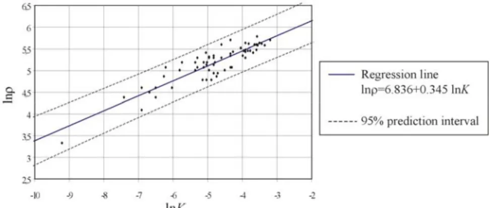
(4) (Belgium). From a dense grid of more than 10 000 cells, 15 hydraulic conductivity values were selected, representing pumping test results in virtual piezometers and providing the hard data set. A regular pattern of sampling locations was rejected for the purpose of keeping consistent with a probable real-world situation.. Fig. 1 (a) Representative cross section and hydraulic conditions of the synthetic aquifer. (b) Distribution of the hydraulic conductivity reference field (lower layer) mapping the 15 virtual piezometers (black dots) and the 12 virtual tomographic profiles (black lines). Both eastern and western constant head boundaries are reported at a distance of 600 m.. A single pumping well (pumping rate of 60 m3 hour-1) located in the heterogeneous sand and gravel unconfined aquifer was used for the simulation. Pure deterministic groundwater flow conditions were then computed, providing the synthetic "measured" heads at the 15 virtual piezometers (first set of soft data).. Fig. 2 Observed correlation between electrical resistivity and hydraulic conductivity (r=0.9) in the alluvial sediments of the Meuse River.. The resistivity data set (second set of soft data) was created based on the observed correlation (r = 0.9) existing between electrical resistivity (ρ) and hydraulic conductivity (K) in the alluvial sediments of the Meuse River (Fig. 2). Considering N (0,1) as a random ) draw within a standard normal distribution and σ , the standard deviation of the regression residual, 300 resistivity values, distributed on 12 tomographic profiles (Fig. 1b) were generated by the following equation:. ) ln ρ = 6.836 + 0.345 ln K + σ N (0,1). (1).
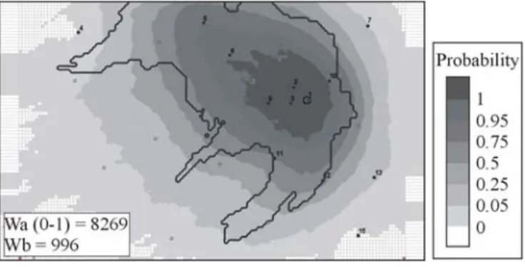
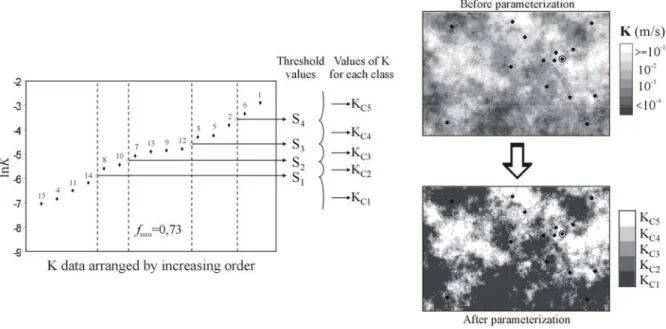
(5) Considering advective transport time to the well, the "true" 20-day isochrone line (associated with the concerned pumping rate) resulting from the "true" hydraulic conductivity field was also computed and used as reference for further comparisons.. Monte Carlo stochastic conditional simulations. The stochastic methodology developed by Varljen & Shafer (1991) is applied in order to determine and quantify the uncertainty in the location and extent of the 20-day capture zone due to imperfect knowledge of the hydraulic conductivity field. According to a Monte-Carlo analysis, four hundred stochastic simulations of equally likely hydraulic conductivity fields for the lower layer were generated using the Turning Bands method. Each of them were subsequently conditioned on hydraulic conductivity measurements by a kriging technique. Groundwater flow and a particle tracking process were computed for each realization. The ensemble of obtained capture zones was then treated statistically to infer the capture zone probability distribution (CaPD). This CaPD gives the spatial distribution of the probability that a conservative tracer particle released at a particular location is captured by the well within a specified time span (van Leewen, 2000), in this particular case 20 days. Figure 3 compares the CaPD with the "real" isochrone and show how the stochastic approach reveals the uncertainty about the location of the protection zone. In order to quantify and evaluate the performance of additional conditioning, two measures among several others have been selected (van Leeuwen et al., 2000). Wa is a measure of uncertainty based on the extent of the uncertainty zone for which the probability P of capture is 0<P<1. Wb compares the location of the reference isochrone with the location of isoline Γ(0.5) for which 50% probability of capture is obtained. Units of both measures are expressed in number of 5 × 5 m cells.. Fig. 3 Comparison of the CaPD determined by realizations conditioned on 15 hydraulic conductivity values, and the reference 20-day isochrone (black line).. Additional conditioning by head measurements (first set of soft data). This additional conditioning was performed by calibrating the groundwater flow on head measurements for each stochastic conditional simulation generated previously by inverse modelling (PEST code, Doherty, 1994). Resolution of the inverse problem required to carry out a parameterisation reducing the number of adjustable parameters. Therefore a zonation (Fig. 4) was applied that consist, based on four specified threshold values (Si), in dividing the hydraulic conductivity variation interval in five classes (Ci) of uniform value (KCi), representing the adjustable parameters. The threshold values were defined by.
(6) determining the best hydraulic conductivity data combination that minimize the variability within each class, by minimizing the following equation: Nc Ndi. (. f = ∑∑ ln K ij − ln K i i =1 j =1. ). 2. with. ln K i =. 1 N di. N di. ∑ ln K j =1. ij. , i = 1, N c. (2). where N c is the number of classes, N di is the number of data in each class (varying from one combination to an other) and. ∑N i. di. = N D , the total number of K data.. Fig. 4 Schematic view of the parameterization technique with the representation of a generated hydraulic conductivity field conditioned on 15 data, before and after the parameterization.. The inverse procedure was applied to optimize the uniform hydraulic conductivity values for each parameter. However, for some realizations, these optimized hydraulic conductivity values did not respect the relative order KCi<KC(i+1) defined by the thresholding. Considering these realizations as geologically erroneous, they were rejected. For each remaining realization, the 20-day capture zone was determined and consequently the CaPD for the ensemble of possible capture zones was estimated (Fig. 5). Results show how the use of head conditioning by inverse modelling combined with the use of a selection criterion reduce the uncertainty of the probability distribution (decrease in Wa)..
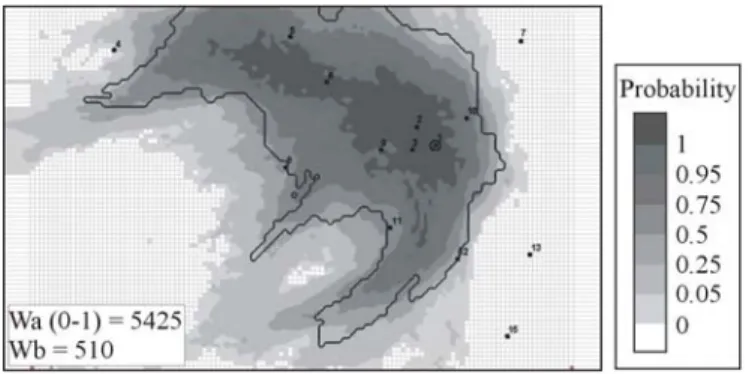
(7) Fig. 5 Comparison of the CaPD determined by realizations conditioned on 15 hydraulic conductivity values and 15 piezometric heads and the reference 20-day isochrone (black line).. Additional conditioning by geoelectrical resistivity data (second set of soft data). The geophysical data set, as additional useful information, was directly integrated in the generation process by conditioning each stochastic simulation on both hydraulic conductivity measurements and resistivity values by a cokriging technique. Four-hundred stochastic "co-conditional" simulations were then generated based on a linear model of coregionalisation that was adjusted on experimental simple and cross-covariances. Following the same procedure as described in the previous paragraph (parameterization and inverse modelling), an advective 20-day isochrone was computed for each remaining realization and the resulting CaPD was calculated (Fig. 6). The use of additional available data decrease the prior uncertainty of the parameters and, in consequence, reduce the uncertainty of the well CaPD (decrease in Wa). It can also be observed that the Γ(0.5) isoline tends to approach the reference isochrone (decrease in Wb). Comparing results of Fig. 6 to those of Fig. 3 (which were found without taking soft data into account), a clear improvement is observed in the description of the medium heterogeneity leading to more realistic isochrones with regards to the reference one.. Fig. 6 Comparison of the CaPD determined by realizations conditioned on 15 hydraulic conductivity values, 15 piezometric heads and 300 resistivity values and the reference 20-day isochrone (black line).. CONCLUSION. Advances in the delimitation of protection zones are made by the use of stochastic methodologies. Moreover introduction of additional available data decreases the prior uncertainty of the parameters and, in consequence, reduces the uncertainty of the well capture zone probability distribution (CaPD). Since geophysical data and head observations are easier to collect on the field than hydraulic conductivity measurements, they are generally more abundant. The methodology presented can be used in real applications to quantify the uncertainty in the location and extent of well capture zones when little or no information is available about the hydraulic properties, through the conditioning on geophysical data and/or head observations. The different stochastic approaches listed previously considers purely advective transport (particle tracking procedure). They do not take the concept of macrodispersivity into account. A topic for further research will be the assimilation of information from solute concentrations (i.e. tracer tests) to further reduce uncertainty in capture zone.
(8) delineation. Further applied research is needed to design optimal strategies of soft data acquisition like, for example, selection of locations for conditioning measurements. Acknowledgements We thank the National Fund for Scientific Research of Belgium for the PhD research grant given to C. Rentier, a part of this work has also been funded through the EU-DAUFIN project (EVK1-1999-00153).. REFERENCES Anderson, M. P. (1997) Characterization of geological heterogeneity. In: Subsurface flow and transport, a stochastic approach (ed. by G. Dagan and S. P. Neuman). International Hydrology Series, 23-43. Bair, E. S., Safreed, C. M. & Stasny, E. A. (1991) A Monte Carlo-based approach for determining traveltime-related capture zones of wells using convex hulls as confidence regions. Groundwater 29(6), 849-855. Beckers, J. & Frind, E. O. (2000) Calibration of the Oro Moraine multi-aquifer system: role of geology and objective function. In: Calibration and Reliability in Groundwater Modelling (ed. by F. Stauffer, W. Kinzelbach, K. Kovar & E. Hoehn), (Proc. Int. Conf. ModelCARE’99, held 20-23 September 1999 in Zűrich, Switzerland), 164-170, IAHS Publ. No. 265. Dassargues, A. (1994) Applied methodology to delineate protection zones around pumping wells. J. Environ. Hydrol. IAEH 2(2), 3-10. De Marsily, G. (1984) Spatial variability of properties in porous media: a stochastic approach. In: Fundamentals of Transport Phenomena in Porous Media (ed. by J. Bear & M. Corapcioglu). 721-769, NATO-ASI Series E(82). Derouane, J. & Dassargues, A. (1998) Delineation of groundwater protection zones based on tracer tests and transport modelling in alluvial sediments. Environ. Geology 36(1-2), 27-36. Doherty, J., Brebber, L. & Whyte, P. (1994) PEST – Model-independent parameter estimation. User's manual. Watermark Computing, Corinda, Australia. Evers, S. & Lerner, D. N. (1998) How uncertain is our estimate of a wellhead protection zone? Groundwater 36(1), 49-57. Feyen, L., Beven, K. J., De Smedt, F. & Freer, J. (2001) Stochastic capture zone delineation within the generalized likelihood uncertainty estimation methodology: Conditioning on head observations. Wat. Resour. Res. 37(3), 625-638. Gelhar, L. W., Welty, C. & Rehfeldt, K. R. (1992) A critical review of data on field-scale dispersion in aquifers. Wat. Resour. Res. 28(7),1955-1974. Gómez-Hernández, J. J., Sahuquillo, A. & Capilla, J. E. (1997) Stochastic simulation of transmissivity fields conditional to both transmissivity and piezometric data, I, Theory. J. Hydrol. 203, 162-174. Guadagnini, A. & Franzetti, S. (1999) Time-related capture zones for contaminants in randomly heterogeneous formations. Groundwater 37(2), 253-260. Kinzelbach, W., Marburger, M. & Chiang, W.-H. (1992) Determination of groundwater catchment areas in two and three spatial dimensions. J. Hydrol. 134, 221-246. Kunstmann, H. & Kinzelbach, W. (2000) Computation of stochastic wellhead protection zones by combining the first-order second-moment method and Kolmogorov backward equation analysis. J. Hydrol. 237, 127-146. Kupfersberger, H. & Blöschl, G. (1995) Estimating aquifer transmissivities – on the value of auxiliary data. J. Hydrol. 165, 8599. Levy, J. & Ludy, E. E. (2000) Uncertainty quantification for delineation of wellhead protection areas using the Gauss-Hermite quadrature approach. Groundwater 38(1), 63-75. Mantoglou, A. & Wilson, J. L. (1982) The turning bands method for simulation of random fields using line generation by a spectral method. Wat. Resour. Res. 18(5), 1379-1394. Mc Kenna, S. A. & Poeter, E. P. (1995) Field example of data fusion in site characterization. Wat. Resour. Res. 31(12), 32293240. Nunes, L. M. & Ribeiro, L. (2000) Permeability field estimation by conditional simulation of geophysical data. In: Calibration and Reliability in Groundwater Modelling (ed. by F. Stauffer, W. Kinzelbach, K. Kovar & E. Hoehn), (Proc. Int. Conf. ModelCARE’99, held 20-23 September 1999 in Zűrich, Switzerland), 117-123, IAHS Publ. No. 265.. Rentier, C., Bouyère, S. & Dassargues, A. (2002) Integrating geophysical and tracer test data for accurate solute transport modelling in heterogeneous porous media. In: Groundwater Quality 2001 (ed. by S. F. Thornton & S. E. Oswald), (Proc. Int. Conf. GQ’2001, held 18-21 June 2001 in Sheffield, UK), 3-10, IAHS Publ. No. 275, pp.. 3-10. Van Leeuwen, M., te Stroet, C. B. M., Butler, A. P. & Tompkins, J. A. (1998) Stochastic determination of well capture zones. Wat. Resour. Res. 34(9), 2215-2223. Van Leeuwen, M., Butler, A. P., te Stroet, C. B. M. & Tompkins, J. A. (2000) Stochastic determination of well capture zones conditioned on regular grids of transmissivity measurements. Wat. Resour. Res. 36(4), 949-957. Van Leeuwen, M. (2000) Stochastic determination of well capture zones conditioned on transmissivity data. PhD thesis, Department of Civil and Environmental Engineering, University of London. Varljen, M. D. & Shafer, J. M. (1991) Assessment of uncertainty in time-related capture zones using conditional simulations of hydraulic conductivity. Groundwater 29(5), 737-748. Vassolo, S., Kinzelbach, W. & Schäfer, W. (1998) Determination of a well head protection zone by inverse stochastic modelling. J. Hydrol. 206, 268-280..
(9)
Figure
Documents relatifs
The coinciding opening of the Central Atlantic Ocean (Biari et al., 2017; Labails et al., 2010) and its propaga- tion toward the Alpine Tethys where extension focused in the
• The shear strain localisation pattern is very similar to the one obtained with the first model in which there is no detachment fault (compare with figure 8.11c-d) : a first
Figure 4 summarizes the proposed development process distinguishing two main roles: the architect, who is assumed to be an expert in the given domain,
Isotopic signatures from the samples of 2008 collected downstream the dams and at the surface of the Masinga reservoir (black diamonds) correlate with 1/DSi, which is consistent with
The documents may come from teaching and research institutions in France or abroad, or from public or private research centers.. L’archive ouverte pluridisciplinaire HAL, est
Comme ´ evoqu´ e en section pr´ ec´ edente, la plupart de ces m´ ethodes sont en r´ ealit´ e ce que nous appelons des m´ ethodes multi-cartes, ou pseudo-volume, ou 2.5-D : le
Ces identités multiples sont aussi le fait de ses jeunes compagnons, dont le marin Yves pourrait être le parangon – honnête père de famille dans Mon frère Yves, accompagnant
• Early astration - According to Piau et al.. Li isotopes in metal-poor halo dwarfs 9 computed by the Big Bang) would have been severely destroyed in the Galaxy before the formation
