HAL Id: halshs-00839147
https://halshs.archives-ouvertes.fr/halshs-00839147
Preprint submitted on 27 Jun 2013
HAL is a multi-disciplinary open access
archive for the deposit and dissemination of sci-entific research documents, whether they are pub-lished or not. The documents may come from teaching and research institutions in France or abroad, or from public or private research centers.
L’archive ouverte pluridisciplinaire HAL, est destinée au dépôt et à la diffusion de documents scientifiques de niveau recherche, publiés ou non, émanant des établissements d’enseignement et de recherche français ou étrangers, des laboratoires publics ou privés.
To cite this version:
Laurent Gobillon, François-Charles Wolff, Patrice Guillotreau. The anatomy of prices on the French fish market. 2013. �halshs-00839147�
The anatomy of prices on the French fish market
Laurent Gobillon
François-Charles Wolff
Patrice Guillotreau
J
EL Codes: L11, Q22
Keywords: Fish, Commodity price, Unobserved heterogeneity,
Variance analysis, Panel data
P
ARIS-
JOURDANS
CIENCESE
CONOMIQUES48, BD JOURDAN – E.N.S. – 75014 PARIS TÉL. : 33(0) 1 43 13 63 00 – FAX : 33 (0) 1 43 13 63 10
www.pse.ens.fr
CENTRE NATIONAL DE LA RECHERCHE SCIENTIFIQUE – ECOLE DES HAUTES ETUDES EN SCIENCES SOCIALES ÉCOLE DES PONTS PARISTECH – ECOLE NORMALE SUPÉRIEURE – INSTITUT NATIONAL DE LA RECHERCHE AGRONOMIQU
The anatomy of prices on the French fish market
Laurent Gobillon
*, François-Charles Wolff
**, Patrice Guillotreau
***June 2013
Abstract
Hedonic price regressions have become a standard tool to study how prices of commodity goods are related to quality attributes. In this paper, we extend the traditional price specification by incorporating three sources of unobserved heterogeneity related to sellers, buyers, and matches between buyers and sellers. The extended price specification is estimated on a unique exhaustive dataset of nearly 15 million transactions occurring in French wholesale fish markets from 2002 to 2007. Results show that unobserved heterogeneity plays a significant role in price formation. For some species, its inclusion in price regressions changes the coefficients of quality-related fish characteristics. Last, using data analysis techniques, we classify fish and crustacean species by the extent to which price variations are related to fish characteristics, time effects and the three sources of unobserved heterogeneity.
Keywords: fish, commodity price, unobserved heterogeneity, variance analysis, panel data JEL Classification: L11, Q22
* Corresponding author. INED, 133 Boulevard Davout, 75980 Paris Cedex 20, France, PSE, CEPR and IZA. E-mail:
laurent.gobillon@ined.fr http://laurent.gobillon.free.fr/
** LEMNA, Université de Nantes, BP 52231, Chemin de la Censive du Tertre, 44322 Nantes Cedex, France and INED, Paris,
France. E-mail: francois.wolff@univ-nantes.fr http://www.sc-eco.univ-nantes.fr/~fcwolff
*** LEMNA and FR CNRS 3473-IUML, Université de Nantes, BP 52231, Chemin de la Censive du Tertre, 44322 Nantes Cedex,
1. Introduction
Hedonic price regressions introduced by the seminal paper of Rosen (1974) have become a widely used approach to study how prices of commodity goods are affected by quality attributes. Each good is characterized by a set of attributes and the unit price of a good is fixed on the market according to supply and demand. The marginal price of every attribute at equilibrium is evaluated from the regression of the unit price on the whole set of attributes. Estimations are usually conducted on cross-section data using Ordinary Least Squares.
A limit of the traditional hedonic approach is that it does not take into account the unobserved heterogeneity of agents. However, prices can be affected by this unobserved heterogeneity as producers can differ in their marginal cost and buyers can differ in their willingness to pay for different products. Moreover, the quality of goods may be partially unobserved as the usual variables measuring quality may not be sufficient to fully describe goods, and the unobserved component of quality may vary across producers.
In fact, the measured effect of observable quality attributes on the price of goods can change when unobserved heterogeneity is taken into account, since goods with specific attributes may be sold by producers with specific marginal costs or bought only by consumers with specific tastes. The involvement of specific producer-seller pairs in transactions may also matter since there may be long-term relationships with discounts, and some information on the unobserved component of the quality of goods sold by some producers may be known only by some buyers.
The main contribution of this paper is to study the role of the unobserved heterogeneity of producers, buyers, and producer-buyer matches in price formation using hedonic price regressions. Our application is on fish, for which we have a unique exhaustive dataset of around 15 million transactions at French wholesale fish auctions over the 2002-2007 period.
Our approach borrows tools from labor economics; since the seminal paper by Abowd, Kramarz and Margolis (1999), a literature has developed incorporating the unobserved heterogeneity of firms and workers in wage regressions through the use of two series of fixed effects. This approach has been expanded to take into account specific effects for pairs of firms and workers (Woodcock, 2008, 2011; Sørensen and Vejlin, 2013). In our paper, we use a similar approach for fish prices per kilo with a specification incorporating fish characteristics, time fixed effects, seller fixed effects, buyer fixed effects and seller-buyer match effects. Identification is guaranteed by the tracking across time of seller and buyer accounts specific to wholesale fish markets.
Our work complements the literature on hedonic price regressions that takes into account, at best, unobserved seller heterogeneity using store fixed effects when retail prices are studied (Lach, 2002). The most significant applications on specific food products mostly concern wine (Nerlove, 1995; Combris, Lecocq and Visser, 1997; Ashenfelter, 2008), cereals (Stanley and Tschirhart, 1991) and fish.
For applications on fish, cross-sectional hedonic price regressions have been used to study ex-vessel prices of fish sold at wholesale auction (McConnell and Strand, 2000; Kristofersson and Rickertsen, 2004, 2007; Asche and Guillen, 2012) and to analyze retail prices in shops to assess the importance of packaging, brand or eco-labelling (Roheim, Gardiner and Asche, 2007; Roheim, Asche and Insignares, 2011).1 Contrary to previous studies on ex-vessel prices which usually focus on one single species or
one single fish market, we provide results for most fish species based on estimations on transactions occurring on all French fish markets.
More precisely, we report regression results without and with unobserved heterogeneity for most of the fish and crustacean species with a significant market share. We also propose a way to classify species by the extent to which fish characteristics and unobserved heterogeneity among sellers, buyers and seller-buyer matches, contribute to explaining fish price variations. Note that we cannot disentangle buyer fixed effects and market effects because we cannot track buyers across markets in our data. However, we provide some hints on the importance of market effects by decomposing variations in buyer effects into variations within and between markets.
Our results show that, for most species, while fish characteristics remain the main determinant of fish prices, heterogeneity among sellers, buyers and matches also contributes to explaining prices. The role of matches remains modest. Interestingly, the inclusion of unobserved heterogeneity in the analysis affects the marginal effect of fish characteristics on prices for several species. This suggests that unobserved heterogeneity terms should be included in regressions as controls to avoid biased estimates of the effect of observable fish attributes.
Data analysis techniques were used to classify fish and crustacean species into four groups. One group comprises species such as sole, monkfish or Norway lobster (live or frozen) for which fish characteristics play an important role in price setting. A second group includes species such as hake, cuttlefish or John Dory, with an explanatory power of buyer and time effects respectively larger and smaller than the average. Conversely, a third group is characterized by an explanatory power of buyer and time effects respectively smaller and larger than the average, and includes lobster, squid, red mullet, seabass (non-line caught), pollack and ling. Finally, the fourth group comprises species such as mackerel, with a larger-than-average explanatory power of time, seller and match effects. Interestingly, the four groups of species differ in the average price per kilo, seasonality and downstream markets.
The rest of the paper is organized as follows. Section 2 describes the empirical strategy used to quantify the importance of fish characteristics, time, seller, buyer and match effects in explaining
1 Controlled experiments have also been used to assess consumers’ willingness to pay for specific fish attributes such as
variations in fish prices. Section 3 presents our dataset of fish transactions along with descriptive statistics. Section 4 comments our results and Section 5 concludes.
2. Empirical strategy
In this section, we explain how unobserved heterogeneity can be incorporated in hedonic price regressions when panel data on fish transactions are available, and sellers and buyers can be tracked across time. We also explain how the role of factors in explaining fish price variations can be quantified.
For a given fish species, we denote by 𝑃𝑖𝑗𝑘𝑡 the log price of a transaction 𝑖 for a fish lot which is sold
by a seller 𝑗 and purchased by a buyer 𝑘 during month 𝑡. We suppose that the logarithm of fish price per kilo across time 𝑃𝑖𝑗𝑘𝑡 depends on a set of fish characteristics 𝑋𝑖 composed of dummies related to
size, presentation and quality. The standard hedonic specification is given by:
𝑃𝑖𝑗𝑘𝑡 = 𝑋𝑖𝛽 + 𝜗𝑡+ 𝜖𝑖𝑗𝑘𝑡 (1)
where 𝛽 is a vector of parameters, 𝜗𝑡 is a month-year fixed effect, and 𝜖𝑖𝑗𝑘𝑡 is a random error term.
This specification is usually estimated with Ordinary Least Squares.
It is possible to add seller unobserved effects 𝛾𝑗 and buyer unobserved effects 𝛿𝑘 to this
specification. In our setting where fish is sold at auctions, seller effects capture all the differences in fish quality across vessels that are not captured by variables in our dataset. We do not have information on vessels such as fishing gear or techniques, but it is unlikely that all the differences in fish quality across vessels would be fully captured with vessel observable attributes even if the related information was available. An advantage of seller unobserved effects is that they capture the effect of all the vessel characteristics without the risk of being non-exhaustive.
Similarly, buyer effects capture all the differences in willingness to pay that can affect prices, as buyers needing fish with specific characteristics are expected to make higher bids for it at auctions. As we will see below when describing the data, buyers cannot be tracked across fish markets.2
Hence, unspecified buyer effects cannot be identified separately from market effects. It should thus be kept in mind that buyer unobserved effects also capture market effects. The specification becomes:
𝑃𝑖𝑗𝑘𝑡 = 𝑋𝑖𝛽 + 𝜗𝑡+ 𝛾𝑗+ 𝛿𝑘+ 𝜖𝑖𝑗𝑘𝑡 (2)
We treat the buyer- and seller-specific components as fixed effects because they may be correlated with the covariates 𝑋𝑖. For instance, vessels fishing very close to coasts and landing their catches
daily sell small quantities of high-quality fresh fish, whereas large vessels operating away from coasts
2 Indeed, in our data, we only have the license codes of accounts used by buyers to purchase fish. These license codes are market-specific and can thus be tracked only within markets.
sell frozen fish in large quantities after several weeks at sea. In the same way, fish traders supplying restaurants will seek to buy high-quality fish, while traders supplying hypermarkets will purchase a broader range of fish species at lower prices.
Specification (2) is a panel data model with two series of non-nested fixed effects. This type of model has been studied in the labor literature since the seminal paper by Abowd, Kramarz and Margolis (1999) who estimate a wage equation with worker and firm fixed effects. Identification of fixed effects is possible only within groups of well-interconnected workers and firms (see Abowd, Creecy and Kramarz, 2002, for more details). Interconnection within a group is ensured because firms employ several workers within the group and enough workers move between firms during the period covered by the data. Groups are mutually exclusive as no worker in a group works for a firm in another group.
By analogy, in our case, identification of fixed effects is possible only within exclusive groups of well-interconnected vessels and buyers. Interconnection within a group is ensured because vessels sell fish to several buyers within the group and buyers purchase from several sellers. We only study the main group of well-interconnected vessels and buyers which, as will be shown, includes nearly all transactions for most species. As there are large numbers of seller and buyer fixed effects in the model, estimations are performed in two steps, as explained in Appendix A.
Next, we introduce in equation (2) the effect of a match between seller 𝑗 and buyer 𝑘, denoted 𝜃𝑗𝑘,
as specific matches can influence fish prices. Indeed, specific vessels sell fish lots of higher quality and this quality is known only by a few customers through bilateral relationships. These customers agree to pay a higher price for the fish lots at auctions. Match effects capture the price premium that some buyers agree to pay to some specific sellers. The resulting model can be decomposed into two equations:
𝑃𝑖𝑗𝑘𝑡 = 𝑋𝑖𝛽 + 𝜗𝑡+ 𝜇𝑗𝑘+ 𝜖𝑖𝑗𝑘𝑡 (3a)
𝜇𝑗𝑘= 𝛾𝑗+ 𝛿𝑘+ 𝜃𝑗𝑘 (3b)
In equation (3a), 𝜇𝑗𝑘 is a seller-buyer fixed effect capturing all the unobserved heterogeneity terms.3
This fixed effect is decomposed in equation (3b) into the seller fixed effect, the buyer fixed effect and the match effect. The identification of the model is extensively discussed in Woodcock (2008, 2011). The accuracy with which a term 𝜇𝑗𝑘 is estimated increases with the number of transactions between
seller 𝑗 and buyer 𝑘. For 𝛾𝑗, 𝛿𝑘 and 𝜃𝑗𝑘 to be separately identified, match effects must be considered
as orthogonal to seller and buyer fixed effects. As before, sellers and buyers must be
3 It would be tempting to simply introduce the match effect in equation (2) as a random effect and take it into account using
standard panel estimation techniques. However, this approach is less general than ours since it does not allow for a correlation between fish characteristics and match effects. Our approach is robust to that issue.
connected, so we again restrict the estimations to the main group of well-interconnected sellers and buyers. The estimation procedure is again detailed in Appendix A.
Our most general specification given by (3a) and (3b) is used to perform a variance decomposition of fish prices. The role of fish characteristics, time, sellers, buyers and matches in explaining variations in fish prices is measured by the ratio between the variance of their effect and the variance of prices. For instance, denote by 𝛽̂ the estimated coefficients of fish characteristics and by 𝑉(∙) the operator giving the variance. The importance of fish characteristics is measured by the ratio 𝑉�𝑋𝑖𝛽̂�/𝑉�𝑃𝑖𝑗𝑘𝑡�.
As a final step, we use these variance ratios to construct groups of species which are similar with respect to their price determinants. We first conduct a Principal Component Analysis (PCA) based on the five variance ratios of fish characteristics, time, seller, buyer and match effects, to assess the dimensions in which species can be distinguished.4 The idea of the approach is to decrease the
number of dimensions in which species are represented from five to a lower number by projecting species on a space of dimension lower than five such that distances between species are only slightly altered by projection. The selected subspace is such that the mean squared distance between projections is as high as possible or, put differently, such that the inertia of the projected cloud of species is maximized.
In fact, it is possible to show that the entire space can be decomposed into axes such that the first one maximizes the inertia of the projection among subspaces of dimension one, the second one maximizes the remaining inertia, and so on (see for instance Jolliffe, 2010). As a result, axes explain a decreasing proportion of the total inertia of the cloud of species. In our application, we will focus on the two first axes as they explain most of the inertia of the cloud of species and thus contain most of the information contained in variance ratios which serves to differentiate species.
We then use an Ascendant Classical Hierarchy (ACH) based on these two first axes to construct groups of similar species. The groups are constructed by consecutive aggregation of subgroups containing one or more species using the Ward distance. The aggregation procedure involves aggregating the two subgroups at each step such that the loss of between-group inertia is minimized, and then repeating the operation until there are only a few subgroups left, and these are our selected groups. In practice, we stop the iterative procedure when four groups are left, as any further reduction in the number of groups leads to a significant loss of between-group inertia.
3. Description of the data
4 As the five variance ratios do not have the same dispersion, we follow the common practice of dividing them by their standard deviation so that they have a comparable influence in the determination of axes when conducting the principal component analysis.
We now give some information on the French fish markets and our dataset on fish transactions. Over the 2002-2007 period, 230,000 tons of fish were landed and sold every year in France, for an average value of 658 million euros and at an average price of 2.85 euros per kilogram (France Agrimer, 2012). The tonnage represents about 30% of total domestically produced seafood when frozen fish and aquaculture products are taken into account, but it represents less than 10% of domestic demand which mostly depends on imports. Fish is traded in markets between vessels and buyers, mostly at auctions in trading rooms, using a mobile electronic clock or by internet (see Guillotreau and Jiménez-Toribio, 2011, for more details).
In France, information on every transaction is collected by the national bureau of seafood products (France Agrimer). This information is then processed into a data system called RIC (Réseau Inter-Criées) and added to a unique dataset that we use in our empirical analysis. This dataset is exhaustive for all transactions on the domestic fresh fish market in France between January 2002 and December 2007.
The data contain a small number of variables providing an accurate description of the transactions. We know the quantity purchased and the total value paid by the buyer, from which we deduce the price paid per kilo. We have the usual detailed characteristics of fish involved in the transaction: species, size, presentation (whole, gutted, in pieces, etc.) and quality measured by freshness (given in descending order from extra to low). The month and year of transactions are recorded but the exact day is not available. We also know whether fish is traded in auction or directly sold to the buyer. Finally, the dataset includes two identifiers, for vessels and buyers respectively. The buyer identifier is a license code corresponding to an account specific to a fish market. A limit of our data is that it is not possible to identify whether several accounts are owned by the same agent. To ease the exposition, we will refer to an account as a buyer, but it should be kept in mind that several accounts on one or several markets may correspond to a single buyer.
Overall, the dataset includes 18,197,738 observations over the 2002-2007 period. We restrict the sample in the following way. First, we exclude transactions with a missing buyer identifier (149,709 observations deleted).5 Second, we delete observations corresponding to direct sales and restrict our
attention to transactions at auctions (909,307 observations deleted).6 Third, we keep only the 49
species for which there are more than 60,000 transactions over the period (2,197,513 observations deleted). Fourth, for each species, we exclude the few incoherent transactions with a negative total value or a negative quantity (30,382 observations deleted) as well as transactions with a price per kilo in the bottom 0.1% or the top 0.1% to avoid potential outliers (63,971 observations deleted).
5 There are missing identifiers only for buyers. The identifier is always given for vessels involved in transactions. 6 We eliminated direct sales because the fish price for such transactions is fixed in a very different way.
Finally, in line with our empirical strategy, for each species we keep the largest group of well inter-connected sellers and buyers, and exclude three species for which this group does not contain most of the observations (282,098 observations deleted).7 For the 46 remaining species, the main group
contains nearly all the transactions. Indeed, the main group accounts for more than 99.6% of transactions for 42 species and the minimum is as high as 95.1%.
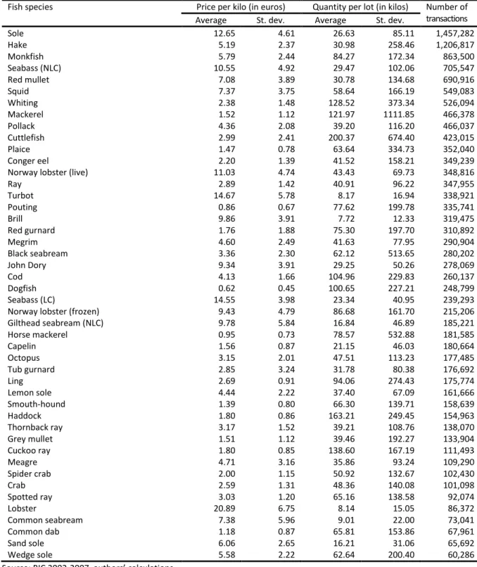
Our selection procedure leaves us with a sample of 14,564,758 transactions of fish and crustaceans belonging to 46 species. According to Table 1, there species are, by decreasing number of transactions: sole, hake, monkfish, seabass (not line-caught), red mullet, squid, whiting, mackerel, Pollack, cuttlefish, plaice, conger eel, Norway lobster (live), ray, turbot, pouting, brill, red gurnard, megrim, black seabream, John Dory, cod, dogfish, seabass (line-caught), Norway lobster (frozen), gilthead seabream (not line-caught), horse mackerel, capelin, octopus, tub gurnard, ling, lemon sole, smouth-hound, haddock, thornback ray, grey mullet, cuckoo ray, meager, spider crab, crab, spotted ray, lobster, common seabream, common dab, sand sole and wedge sole.
[ Insert Table 1 here ]
According to Figure 1, which gives the contribution of each fish species to the total market value, trade is concentrated on a limited number of species. The two main species, sole and monkfish, represent 26.9% of total value. The first five species represent 44.2% of the total market and the first ten species 66.7%.
[ Insert Figure 1 here ]
Table 1 shows considerable heterogeneity in the average price per kilo and the average quantity involved in transactions across species. The most expensive species is lobster, with a price per kilo around 21 euros. There are several very cheap species, such as mackerel, with a price per kilo below 2 euros. The correlation between the average quantity per lot and the average price is negative at -0.50. Whereas the average quantity per lot is as low as 8.1 kilos for lobster, it reaches 122.0 kilos for mackerel and peaks at 200.4 kilos for cuttlefish. In fact, the size of lots sold at auction can vary considerably. The standard deviation for average quantity per lot is highest for mackerel at 1111.9 kilos.
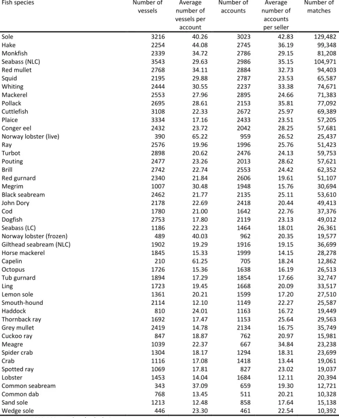
Table 2 sheds some light on the market structure. The numbers of buyers and sellers vary considerably across species. Among species with a significant market share, there are around 3200 vessels selling to 3000 buyers for sole, but only 400 vessels selling to 1000 buyers for Norway lobster (live). The correlation between numbers of buyers and sellers is 0.88. What matters in our empirical application is the degree of interconnection between the two. It can be crudely assessed from the
7 The three fish species excluded from the sample are sardine (114,784 transactions), white seabream (75,279 transactions)
and anchovy (72,884 transactions). For each of these three species, the share of transactions in the main group is 53.8%, 61.1% and 76.3%, respectively. For the remaining 46 species, only 19,151 transactions are excluded because they are not in the main group.
number of buyers per seller and the number of sellers per buyer. For all species in our sample, there is a very good inter-connection between sellers and buyers. For instance, for sole, each vessel sells fish to 43 buyers on average, and each buyer purchases fish from 40 sellers on average. The two numbers exceed 12 for all species. The average number of buyers per seller is 23 and the average number of sellers per buyer is 25.
[ Insert Table 2 here ]
A match is defined as a seller-buyer pair involved in at least one transaction. The number of matches varies a great deal across species. Among species with a significant market share, there are 129,482 matches for sole, but only 25,437 for Norway lobster (live). The minimum for all species is 10,328 and the average is 44,231. The correlations between number of matches and numbers of sellers and buyers are, respectively, 0.82 and 0.88. The estimation accuracy of match effects depends on the number of transactions per match. Figure 2 gives statistics on the number of transactions per match for every species. The first decile is 2 or above for all species except two (grey mullet and lobster). The median is quite high as it takes a value of 8 or above for all species. Finally, the ninth decile is above 30 for all species and reaches a maximum for sole at 144.
[ Insert Figure 2 here ]
4. Empirical results
4.1. Hedonic prices regressions Coefficient estimates
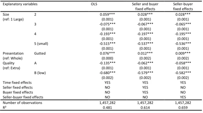
In Table 3, we report results of hedonic price regressions for the two species which have by far the highest market shares, sole and monkfish. Estimation results are given for three specifications: one without unobserved heterogeneity (equation 1), one including additive seller and buyer fixed effects (equation 2), and one including seller-buyer fixed effects (equation 3a).
[ Insert Table 3 ]
In Panel A for sole, column 1 corresponds to the Ordinary Least Squares estimates when fish characteristics and month dummies are introduced.8 The R² is 0.481, meaning that observable fish
characteristics and time explain as much as 48.1% of price variations. The coefficients of fish characteristics have the expected sign. While small fish (sizes 4 and 5, and to a lesser extent size 3) is cheaper than large fish (size 1), medium-sized fish (size 2) is the most expensive. Medium-sized fish is
8 The quantity of fish purchased is excluded from the specification. Indeed, it is potentially endogenous since fish lot sizes
may be influenced by the expected selling price. Still, we conducted a robustness check to assess whether adding the logarithm of fish quantity to our specification affects the results. Whereas this variable is found to have a significant negative effect, its inclusion has absolutely no effect on the magnitude of the coefficients of fish characteristics and does not improve the fit of the model. For sole, for instance, the R² increases only at the margin from 0.4814 to 0.4818 when adding fish quantity to the set of explanatory variables.
6.1% more expensive than large fish, but the smallest fish is 40% less expensive.9 Results are
consistent with medium-sized fish being the most valued. Presentation significantly influences price per kilo. Low-quality fish (grade B) is 45.6% cheaper than extra-quality fish (grade E). Gutted fish is 7.9% more expensive than whole fish because non-edible parts have been eliminated.
Month-year effects are represented in Figure B1 in Appendix B. There is an upward trend over time consistent with inflation. Prices also exhibit seasonality effects, fish being more expensive during summer holidays (July and August) and in December when demand is higher during the Christmas and New Year period.
We then estimate a specification where seller and buyer fixed effects have been added. Results reported in column (2) show a significant improvement of the fit with an increase of the R² from 0.481 to 0.614. This suggests some heterogeneity among vessels and buyers. Some coefficients of fish characteristics change when seller and buyer fixed effects are included in the model, but the results remain qualitatively similar. In particular, the price of gutted fish is now only 1.2% higher than that of whole fish.
Finally, we consider a hedonic price specification with seller-buyer fixed effects. Results reported in column 3 show that the fit improves, with the R² increasing from 0.614 to 0.659. This increase may seem rather modest, but the contribution of match effects to explaining variations in fish prices is significant, accounting for 25.3% of the overall contribution of unobserved heterogeneity terms.10
The introduction of seller-buyer fixed effects instead of seller and buyer fixed effects does not have much effect on the coefficients of fish characteristics.11
Results obtained for monkfish are reported in Panel B and lead to quite similar overall conclusions. Ordinary Least Squares estimates show that prices are higher for fish which is larger, of better quality, or sold in pieces. As shown in Figure B2 in Appendix B, there is an upward time trend and a seasonal effect, with fish being more expensive in December. Introducing seller and buyer fixed effects in a standard hedonic price regression increases the R² from 0.582 to 0.693. Introducing seller-buyer fixed effects instead of seller and buyer fixed effects increases the R² to 0.734. Hence, all sources of unobserved heterogeneity contribute to explaining price variations. Estimated coefficients of fish characteristics are influenced by the presence of unobserved heterogeneity. In particular, whereas gutted fish is 4.7% cheaper than whole fish when the specification does not contain any heterogeneity term, it is found to be 16% more expensive when seller and buyer fixed effects are added.
9 These percentages are given by (exp(0.059)-1)*100 and (exp(-0.515)-1)*100, respectively. Other percentages in the text
are computed in the same way.
10 This percentage is computed as (0.659-0.614)/(0.659-0.481)*100.
11 The profile of time effects when all sources of unobserved heterogeneity are introduced is given in an appendix external
to the paper available upon request. It is nearly confounded with the one obtained when no source of unobserved heterogeneity is introduced.
We estimate hedonic price regressions for every species to obtain systematic conclusions about the importance of unobserved heterogeneity in explaining variations in fish prices.12 Interestingly, the
introduction of unobserved heterogeneity changes the effect of some fish characteristics in a sizable way for several species. For cuttlefish in particular, whereas low quality fish (grade B) is 30.0% less expensive than extra quality fish (grade E) when unobserved heterogeneity terms are omitted, it is only 10.8% less expensive when seller and buyer fixed effects are introduced. There is a similar pattern for hake, the respective figures being 50.5% and 38.6%. For cod, whereas fillets are 63.7% more expensive than whole fish when unobserved heterogeneity terms are omitted, they are only 18.3% more expensive when seller and buyer fixed effects are introduced.
For Norway lobster (frozen), it is the opposite, with pieces being 53.2% less expensive than whole lobster when unobserved heterogeneity is omitted, but only 37.6% less expensive when seller and buyer fixed effects are introduced into the regression. Differences can be explained by some unobserved heterogeneity among sellers correlated both with the presentation category and unobserved fish quality, as vessels use different types of fishing gear. They can also be explained by some unobserved heterogeneity among buyers in the willingness to pay, correlated with presentation category, as there are different types of buyers such wholesalers, multiple grocers or mongers, and different downstream markets where buyers resell fish.
Price variations explained by fish characteristics and unobserved heterogeneity terms
We also evaluate the explanatory power of unobserved heterogeneity terms for each species. Figure 3 reports, for each species, the R² obtained when unobserved heterogeneity is not taken into account, the R² increase when seller and buyer fixed effects are added to the specification, and the R² increase when seller-buyer fixed effects are considered instead of seller and buyer fixed effects. The R² obtained when unobserved heterogeneity is not taken into account is quite high, with an average of 0.47, but it varies across species. Among species with a significant market share, it is only 0.27 for the mackerel, but it reaches 0.70 for Norway lobster (frozen).
[ Insert Figure 3 ]
The explanatory power of seller and buyer fixed effects is relatively high as well, since the R² increases on average by 0.20 when they are introduced in the regression. The R² increase varies across species, from as little as 0.06 for seabass (line-caught), up to 0.37 for cuttlefish. Finally, the explanatory power of match effects is significant, but not large. When introducing seller-buyer fixed effects instead of seller and buyer fixed effects in the regression, the R² increases on average by 0.06. The R² increase is only 0.02 for Norway lobster (live or frozen), but reaches 0.11 for ling.
4.2. Variance analysis of fish prices for all species
Explanatory power of fish, seller, buyer and match effects
Another way to assess the importance of the different factors in explaining fish price variations is to conduct a variance analysis of the most general specification including fish characteristics, time fixed effects, seller fixed effects, buyer fixed effects and match effects.13 Table 4 reports, for every factor,
the ratio between the variance of its effect and the variance of fish prices.14 The higher the variance
ratio of an effect, the higher the explanatory power of the related factor.
As expected, the explanatory power of fish characteristics is high, as the average variance ratio for fish characteristics is 31.9%. There are large variations across species: this ratio is only 7.9% for squid, but 61.1% for Norway lobster (frozen). Time fixed effects have a lower explanatory power, but it is still significant, as the average variance ratio for time fixed effects is 10.4%. This ratio is very large for some specific species with seasonal demand. For instance, the ratio is 33.2% for lobster, which is consumed in large quantities in summer and in December, but less during the rest of the year. Overall, unobserved heterogeneity has a high explanatory power for many species, the average variance ratio for the sum of all the unobserved heterogeneity terms being 29.2%. Buyer heterogeneity is the main unobserved factor affecting prices. In particular, the variance ratio of buyer effects is larger than that of seller effects for all species, and it is larger than that of match effects for all species except one. The average variance ratio of buyer effects is 20.7%. The ratio is low for cuckoo ray and seabass (line-caught), at 4.2% and 5.2%, respectively, but very high for cuttlefish, at 43.6%. By contrast, the average variance ratio of seller effects is only 5.2%. It is very low for some species such as Norway lobster (live) for which it is only 1.5%, but it is quite high for other species such as crab and octopus, at 14.6% and 15.2%, respectively. Finally, the average variance ratio of match effects is 6.2%, with some variations across species. It is quite low for Norway lobster (frozen) at 2.1%, but reaches 10.6% for ling.
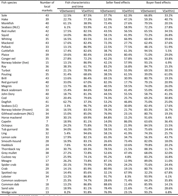
Decomposition of variances within and between fish markets
We now assess to what extent fish prices are related to local markets by further decomposing variations of fish, seller and buyer effects into variations within and between fish markets.15 For fish
and seller effects, variations between fish markets correspond to spatial differences, respectively, in
13 Match effects are obtained by further estimating equation (3b), as explained in Appendix A.
14 Note that ratios do not sum to 1. This is because covariances between the different types of effects are not equal to zero.
For the sake of brevity, we did not report covariances, but they are available upon request.
15 We do not present any decomposition for match effects as their average in each market is zero by construction. This
occurs because one of our identification conditions given in Section 3 is equivalent to match effects being orthogonal to buyer dummies. This yields that the average of estimated match effects for each buyer is zero. As the average of match effects in a market is a weighted average of mean match effects computed for each buyer on that market, the average of match effects in that market is zero.
observed quality measured by size, presentation and quality grade, and in unobserved quality related to fishing practices. For buyer effects, variations capture both spatial differences in the local composition of buyers with respect to their willingness to pay, and differences between local market effects. Note that we cannot disentangle these two sources of variations as accounts are market-specific and the identity of buyers with accounts on several markets is not available.
Table 5 reports the shares of within- and between-market variance for fish, seller and buyer effects for every species. For the effect of fish characteristics, most variations occur within markets, as only 20.8% of variations can be attributed, on average, to differences between markets. Spatial differences are larger for some species, such as monkfish, for which the share of between-market variance reaches 61.1%. They are very small for some others, such as seabass (line-caught), for which the share of between-market variance is only 3.3%.
For seller effects, more than half of variations occur between markets, as the average share of between-market variance is 59.4%. This suggests significant variations in fish practices across space. There are large differences between species as the share of between-market variance reaches 95.2% for cuckoo ray, but only 19.6% for plaice. Finally, for buyer effects, most of variations occur between fish markets as the share of between-market variance reaches 73.4%. This can be explained by the sorting of buyers across space according to their willingness to pay, the strong influence of local markets, or both. There are differences between species, with the share of between-market variance ranging from 94.5% for cuttlefish to just 48.1% for pollack.
[ Insert Table 5 here ]
Robustness checks
In our approach, a match effect is estimated as the average of price residuals at the match level once fish, seller and buyer effects have been netted out (see Appendix A for more details). When there is only one transaction for a match, the estimated match effect is the single price residual. It becomes clear that there is an identification issue as the estimated match effect captures both the true match effect and the noise specific to the price of the transaction. As a robustness check, we replicated our analysis considering only transactions for matches with at least 2, 5 or 10 transactions, as this should alleviate identification problems at the expense of making a non-random selection on transactions.16
We now contrast our baseline results on the explanatory power of the different factors measured by their variance ratio with those obtained when restricting the sample to transactions in matches involving at least 5 transactions. We find that the explanatory power of matches is smaller as the average variance ratio of match effects decreases from 6.2% to 2.4%. This decrease can be explained
by an attenuation of noise in our measure of match effects or a selection effect such that transactions for specific matches with a small number of transactions with extreme prices have been discarded from the sample. In fact, the variance ratio of match effects is small for all species as it is always below 2.5%.17 Considering only transactions for matches with at least 10 transactions in the
estimations gives similar qualitative results, although variance ratios of match effects are now even smaller as their average is 1.5%.
4.3. A classification of fish and crustacean species
As a last step in our analysis, we attempt to construct groups of fish and crustacean species which are similar with respect to their price determinants. We first conduct a principal component analysis to identify the dimensions in which fish and crustaceans differ. We use five variables, which are the variance ratios of fish characteristics, time effects, seller effects, buyer effects and match effects, and whose values are reported in Table 4.18
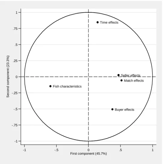
Results are summarized in Table 6 and the two main axes of the principal component analysis are represented in Figure 4.19 The first axis is by far the main dimension in which species differ, as it
explains a full 46% of the inertia of the cloud of species. It opposes fish characteristics to the unobservables related to sellers, buyers and matches. This opposition is driven by the large negative correlations between the effects of fish characteristics and match effects (-0.68), seller effects (-0.43) and buyer effects (-0.43). The second axis has less importance, explaining less than 23% of the inertia of the cloud of species. It mostly opposes time effects and buyer effects, the correlation between these two types of effects being rather low, at -0.17.
[ Insert Table 6 here ] [ Insert Figure 4 here ]
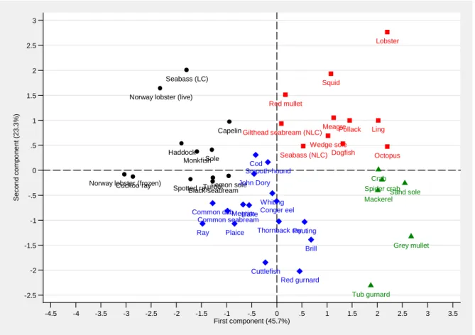
We then use the positions of species on the first two axes in an ascendant classical hierarchy to construct groups of species with similar price determinants. We consider a classification with four groups which are represented in Figure 5.20 Most species in the first group have negative values on
the first axis and fish characteristics usually have a large explanatory power. The variance ratio of fish
17 Another noticeable difference with our baseline results is that the variance ratios of vessel and buyer effects are now
simultaneously significantly larger for mackerel, red gurnard, horse mackerel and mullet, whereas the variance ratio of the sum of all the unobserved heterogeneity terms is smaller. These contrasting results cannot be explained by the decrease in the variance ratio of match effects as it is too small to compensate for the increase in the variance ratios of vessel and buyer effects. However, they can be explained by an increase in the negative correlation between vessel fixed effects and buyer fixed effects in absolute terms. Even if the variance ratios of vessel and buyer effects are larger, the variance ratio of their sum does not need to be larger as the negative correlation between vessel and buyer fixed effects has increased.
18 Horse mackerel is excluded from the analysis because it looks like an outlier (its variance ratio of buyer effects is very high
at 83.7%). Furthermore, its market share is very low.
19 Appendix C reports the coordinates of species on the two first axes, as well as their contributions and some projection
information.
characteristics is 44.6% on average in this group, compared to 32.4% for the whole sample of species. Unobserved heterogeneity does not play much of a role for most species in this group. The average variance ratios of seller, buyer and match effects are all below the averages computed for the whole sample of species. In particular, the group contains sole, monkfish, Norway lobster (live or frozen), seabass (line-caught), turbot and haddock. Most species are expensive (around 10€/kg) and highly differentiated across presentation categories, consistent with an important role of fish characteristics in price formation. For instance, Norway lobsters are less valued when frozen rather than alive, except the largest ones, monkfish is more valued whole rather than beheaded, and portion-size soles (ie. size 2) are the most appreciated.
Most species in the second group have negative values on the second axis. Time effects usually have a low explanatory power and buyer effects have an explanatory power slightly above average. The average variance ratios of time and buyer effects are respectively 5.6% and 22.2%, compared to 10.5% and 19.3% for the whole sample of species. This group includes hake, cuttlefish, John Dory, cod, ray, plaice and conger eels. These species have a low price (around 4€ per kilo) which is not subject to seasonal variability as fish is caught the whole year and is purchased mostly by wholesalers. Willingness to pay differs among buyers depending on their downstream markets. Indeed, marketing efforts (such as discounted prices and advertising) are sometimes considerable as these species are of low value and the profits buyers can derive from sales vary across downstream customers.
Nearly all species in the third group have positive values on both the first and second axis, and are characterized by a large explanatory power of time effects and a slightly below average explanatory power of seller and match effects. In particular, time effects have an average variance ratio of 18.3% compared to 10.5% for the whole sample of species. This group includes lobster, squid, red mullet, seabass (non-line caught), pollack and ling. With the noticeable exception of lobster which is caught in traps, all these species sell at around 7€ per kilo and are caught seasonally by pelagic trawlers. For lobster, consumers' willingness to pay varies seasonally and is highest during summer and the Christmas holidays.
Finally, the fourth group is characterized by a high explanatory power of buyer, seller and match effects. The variance ratios of these three types of effects are respectively 30.0%, 9.1% and 8.3%, compared to 19.3%, 5.0% and 6.2% for the whole sample of species. The only species in that group with a significant market share is mackerel. This low-value species is mainly harvested in the English Channel by trawlers and sold to wholesalers who export it frozen or canned to foreign markets where it is sold at rather cheap prices. It is also caught by small-scale vessels (such as purse-seiners, gill-netters or liners) and sold to wholesalers who resell it on retail markets for higher prices. This may explain the high variance ratios of the three unobserved heterogeneity terms, as large trawlers
and small-scale vessels differ in their production costs, sellers differ in their willingness to pay depending on how products are presented on the downstream markets, and there can be specific matches depending on the segment of the downstream market involved.
To sum up, the sample of species can be divided into group 1 for which the variance ratio of fish characteristics is significantly above average, and groups 2, 3 and 4 for which different combinations of variance ratios of time, seller and buyer effects deviate significantly from the average. Interestingly, groups of species differ in their average price per kilo, seasonality and downstream markets.
[ Insert Table 7 here ] [ Insert Figure 5 here ]
5. Conclusion
In this paper, we have shown how the unobserved heterogeneity of sellers, buyers, as well as matches between sellers and buyers, can be simultaneously taken into account in hedonic price regressions. Estimations are conducted separately for most fish and crustacean species with a significant market share using a unique exhaustive dataset containing some information on all transactions occurring in French fish markets over the 2002-2007 period. Our work contrasts with the literature, as the typical study usually focuses on one single species or one single fish market, and regresses fish prices on a set of observable characteristics related to fish quality.
When unobserved heterogeneity terms are included in hedonic price regressions, the effects of quality-related fish characteristics change significantly for some species. For almost all species, observable fish characteristics are found to have the largest explanatory power, but the explanatory power of seller, buyer and match effects is also significant. We finally propose a classification of fish and crustacean species depending on the explanatory power of observables and unobservables using a principal component analysis followed by an ascendant classical hierarchy. This classification tends to differentiate species by their value, seasonality and downstream markets.
A limit of our approach is that we cannot distinguish market effects from buyer effects because buyers cannot be tracked across markets. A decomposition of the variance of buyer effects within and between markets shows that market effects could be large. Future research could try to assess the importance of market effects using a dataset tracking buyers across markets. Once market effects net of all sources of heterogeneity are recovered, additional exercises can be conducted, such as testing the law of one price across markets or assessing the extent to which market structure can affect local prices.
References
Abowd J., Kramarz F., Margolis D., (1999), “High wage workers and high wage firms”, Econometrica, vol. 67, pp. 251-233.
Abowd J., Creecy R., Kramarz F., (2002), “Computing person and firm effects using linked longitudinal employer-employee data”, mimeo, Cornell University.
Alfnes F., Guttormsen A., Steine G., Kolstad K., (2006), “Consumers’ willingness to pay for the color of salmon: A choice experiment with real economic incentives”, American Journal of Agricultural
Economics, vol. 88, pp. 1050-1061.
Asche F., Guillen J., (2012), “The importance of fishing method, gear and origin: The Spanish hake market”, Marine Policy, vol. 36, pp. 365-369.
Ashenfelter O., (2008), “Predicting the quality and prices of Bordeaux wine”, Economic Journal, vol. 118, F175-F184.
Card D., Krueger A., (1992), “School quality and black-white relative earnings: a direct assessment”,
Quarterly Journal of Economics, vol. 107, pp. 151-200.
Combris P., Lecocq S., Visser M., (1997), “Estimation of a hedonic price equation for Bordeaux Wine: does quality matter?”, Economic Journal, vol. 107, pp. 390-402.
France Agrimer, (2012), Les filières pêche et aquaculture en France, chiffres-clés, Paris, 36 p.
Guillotreau P., Jiménez-Toribio R., (2011), “The price effect of expanding fish markets”, Journal of
Economic Behavior and Organization, vol. 79, pp. 211-225.
Jolliffe I. (2010), “Principal Component Analysis”, 2nd edition, Springer-Verlag, New York, 487p.
Kristofersson D., Rickertsen K., (2004), “Efficient estimation of hedonic inverse input demand systems”, American Journal of Agricultural Economics, vol. 86, pp. 1127-1137.
Kristofersson D., Rickertsen K., (2007), “Hedonic price models for dynamic markets”, Oxford Bulletin
of Economics and Statistics, vol. 69, pp. 387-412.
Lach S., (2002), “Existence and persistence of price dispersion: An empirical analysis”, Review of
Economics and Statistics, vol. 84, pp. 433-444.
McConnell K., Strand I., (2000), “Hedonic prices for fish: Tuna prices in Hawaii”, American Journal of
Agricultural Economics, vol. 82, pp. 133-144.
Nerlove M., (1995), “Hedonic price functions and the measurement of preferences: the case of Swedish Wine Consumers”, European Economic Review, vol. 39, pp. 1697-1716.
Roheim C., Asche F., Insignares J., (2011), “The elusive price premium for ecolabelled products: Evidence from seafood in the UK market”, Journal of Agricultural Economics, vol. 62, pp. 655-668. Roheim C., Gardiner L., Asche F., (2007), “Value of brands and other attributes: Hedonic analysis of retail frozen fish in the UK”, Marine Resource Economics, vol. 22, 239-253.
Rosen S., (1974), “Hedonic prices and implicit markets: product differentiation in pure competition”,
Journal of Political Economy, vol. 88, pp. 34-55.
Sørensen T., Vejlin R., (2013), “The importance of worker, firm and match effects in the formation of wages”, Empirical Economics, forthcoming.
Stanley L.R., Tschirhart J., (1991), “Hedonic prices for a non-durable good: The case of breakfast cereals”, Review of Economics and Statistics, vol. 73, pp. 537-541.
Woodcock S.D., (2008), “Wage differentials in the presence of unobserved worker, firm, and match heterogeneity”, Labour Economics, vol. 15, pp. 771-793.
Figure 1. Contributions of fish and crustacean species to total market value
Source: RIC 2002-2007, authors’ calculations. Note: NLC = not line-caught, LC = line-caught.
0 5 10 15 C o nt ri b ut ion ( in % ) S ol e M o n kf ish S qu id S e ab as s ( N LC ) H ak e C u ttl e fi s h N or w a y l ob s ter ( fr oz en ) N o rw a y lo b st e r ( live ) W hi ti ng R ed m u llet C od S ea ba s s ( LC ) J oh n D o ry P o lla c k M e gr im M a c k er el H ad do c k L ing T ur bo t R ay P la ic e B lac k s e ab re am C uc k o o ra y G ilt he ad s ea br ea m ( N L C ) C on ge r ee l B rill R ed g ur na rd O c top us Le m on s ol e P o ut ing W ed ge s ol e S po tt ed r ay S m o ut h-ho un d L ob s ter M ea gr e H or s e m a c k er el T h or nb ac k r a y D o g fi s h C ra b S pi d er c ra b T u b gu rn ar d G rey m u llet S an d s o le C ap el in C om m o n da b C om m o n s e ab re am
Figure 2. Number of transactions per match
Source: RIC 2002-2007, authors’ calculations. Note: NLC = not line-caught, LC = line-caught.
0 50 100 150 N um b er o f tr an s a c ti on s pe r m at c h S ol e H ak e M o n kf ish S e ab as s ( N LC ) R ed m u llet S qu id W hi ti ng M a c k er el P o lla c k C u ttl e fi s h P la ic e C on ge r ee l N o rw a y lo b st e r ( live ) R ay T ur bo t P o ut ing Brill R ed g ur na rd M e gr im B lac k s e ab re am J oh n D o ry C od D o g fi s h S ea ba s s ( LC ) N or w a y l ob s ter ( fr oz en ) G ilt he ad s ea br ea m ( N L C ) H or s e m a c k er el C ap el in O c top us T u b gu rn ar d L ing Le m on s ol e S m o ut h-ho un d H ad do c k T h or nb ac k r a y G rey m u llet C uc k o o ra y M ea gr e S pi d er c ra b C ra b S po tt ed r ay L ob s ter C om m o n s e ab re am C om m o n da b S an d s o le W ed ge s ol e P10 - P90 Median Mean
Figure 3. Differences in model goodness of fit
Source: RIC 2002-2007, authors’ calculations.
Note: NLC = not line-caught, LC = line-caught. “OLS R²” gives the R-square of a specification without any unobserved heterogeneity terms related to sellers and buyers, which is estimated with OLS. “seller and buyer fixed effects R²” gives the square of a specification additionally including seller and buyer fixed effects. “seller-buyer fixed effects R²” gives the R-square of a specification including seller-buyer fixed effects, but not seller and buyer fixed effects.
0 .2 .4 .6 .8 R² S ol e H ak e M o n kf ish S e ab as s ( N LC ) R ed m u llet S qu id W hi ti ng M a c k er el P o lla c k C u ttl e fi s h P la ic e C on ge r ee l N o rw a y lo b st e r ( live ) R ay T ur bo t P o ut ing Brill R ed g ur na rd M e gr im B lac k s e ab re am J oh n D o ry C od D o g fi s h S ea ba s s ( LC ) N or w a y l ob s ter ( fr oz en ) G ilt he ad s ea br ea m ( N L C ) H or s e m a c k er el C ap el in O c top us T u b gu rn ar d L ing Le m on s ol e S m o ut h-ho un d H ad do c k T h or nb ac k r a y G rey m u llet C uc k o o ra y M ea gr e S pi d er c ra b C ra b S po tt ed r ay L ob s ter C om m o n s e ab re am C om m o n da b S an d s o le W ed ge s ol e
Figure 4. Principal component analysis of variance decomposition of fish prices
Source: RIC 2002-2007, authors’ calculations.
Fish characteristics Time effects Seller effects Buyer effects Match effects -1 -.75 -.5 -.25 0 .25 .5 .75 1 S ec on d c o m po ne nt ( 23 .3 % ) -1 -.5 0 .5 1 First component (45.7%)
Figure 5. Classification of fish and crustacean species obtained from the Ascendant Classical Hierarchy
Source: RIC 2002-2007, authors’ calculations.
Note: group 1 is represented by black dots, group 2 by blue diamonds, group 3 by red squares and group 4 by green triangles.
Black seabream Norway lobster (frozen)
Norway lobster (live)
Lemon sole Capelin Seabass (LC) Cuckoo ray Sole Monkfish
Spotted rayTurbot Haddock
Brill Hake
Ray
Megrim Conger eel
Red gurnard Cod Cuttlefish Pouting Common seabream Smouth-hound Common dab John Dory Plaice Whiting Thornback ray Meagre Octopus Lobster Seabass (NLC) Gilthead seabream (NLC) Squid Pollack Ling Dogfish Red mullet Wedge sole Sand sole Tub gurnard Grey mullet Spider crab Mackerel Crab -2.5 -2 -1.5 -1 -.5 0 .5 1 1.5 2 2.5 3 S ec on d c o m po ne nt ( 23 .3 % ) -4.5 -4 -3.5 -3 -2.5 -2 -1.5 -1 -.5 0 .5 1 1.5 2 2.5 3 3.5 First component (45.7%)
Table 1. Descriptive statistics on transactions by species
Fish species Price per kilo (in euros) Quantity per lot (in kilos) Number of transactions Average St. dev. Average St. dev.
Sole 12.65 4.61 26.63 85.11 1,457,282 Hake 5.19 2.37 30.98 258.46 1,206,817 Monkfish 5.79 2.44 84.27 172.34 863,500 Seabass (NLC) 10.55 4.92 29.47 102.06 705,547 Red mullet 7.08 3.89 30.78 134.68 690,916 Squid 7.37 3.75 58.64 166.19 549,083 Whiting 2.38 1.48 128.52 373.34 526,094 Mackerel 1.52 1.12 121.97 1111.85 466,378 Pollack 4.36 2.08 39.20 116.20 466,037 Cuttlefish 2.99 2.41 200.37 674.40 423,015 Plaice 1.47 0.78 63.64 334.73 352,040 Conger eel 2.20 1.39 41.52 158.21 349,239 Norway lobster (live) 11.03 4.74 43.43 69.73 348,816 Ray 2.89 1.42 40.91 96.22 347,955 Turbot 14.67 5.78 8.17 16.94 338,921 Pouting 0.86 0.67 77.62 199.78 335,741 Brill 9.86 3.91 7.72 12.33 319,475 Red gurnard 1.76 1.88 75.30 197.70 310,892 Megrim 4.60 2.49 41.63 77.95 290,904 Black seabream 3.36 2.30 62.12 513.65 280,202 John Dory 9.34 3.91 29.25 50.26 278,069 Cod 4.13 1.66 104.96 229.83 260,137 Dogfish 0.62 0.45 100.65 227.21 248,799 Seabass (LC) 14.55 3.98 23.34 40.95 239,293 Norway lobster (frozen) 9.43 4.79 86.68 161.70 215,206 Gilthead seabream (NLC) 9.78 5.84 16.84 46.89 185,221 Horse mackerel 0.95 0.73 78.57 532.88 181,585 Capelin 1.56 0.87 21.15 46.03 180,664 Octopus 3.15 2.01 47.51 113.23 177,485 Tub gurnard 2.85 3.24 31.78 80.38 176,692 Ling 2.69 0.91 94.06 274.43 175,774 Lemon sole 4.44 2.22 37.40 67.09 161,666 Smouth-hound 1.39 0.80 66.30 139.71 158,639 Haddock 1.80 0.86 163.21 249.45 154,963 Thornback ray 3.17 1.52 39.21 108.76 138,070 Grey mullet 1.51 1.12 39.46 192.27 133,904 Cuckoo ray 1.80 0.85 138.60 167.19 111,493 Meagre 4.71 3.16 35.86 93.24 109,290 Spider crab 2.00 1.15 50.92 132.67 102,430 Crab 2.59 1.31 48.36 140.08 101,098 Spotted ray 3.03 1.20 65.16 138.58 92,074 Lobster 20.89 6.75 8.14 15.05 86,372 Common seabream 7.38 5.96 9.01 22.00 73,041 Common dab 1.18 0.87 65.81 153.86 67,961 Sand sole 6.06 2.65 16.21 31.06 65,692 Wedge sole 5.58 2.22 62.64 200.40 60,286 Source: RIC 2002-2007, authors’ calculations.
Table 2. Descriptive statistics of the market
Fish species Number of
vessels number of Average vessels per account
Number of
accounts number of Average accounts per seller Number of matches Sole 3216 40.26 3023 42.83 129,482 Hake 2254 44.08 2745 36.19 99,348 Monkfish 2339 34.72 2786 29.15 81,208 Seabass (NLC) 3543 29.63 2986 35.15 104,971 Red mullet 2768 34.11 2884 32.73 94,403 Squid 2195 29.88 2787 23.53 65,587 Whiting 2444 30.55 2237 33.38 74,671 Mackerel 2553 27.96 2895 24.66 71,383 Pollack 2695 28.61 2153 35.81 77,092 Cuttlefish 3108 22.33 2672 25.97 69,389 Plaice 3334 17.16 2433 23.51 57,205 Conger eel 2432 23.72 2042 28.25 57,681 Norway lobster (live) 390 65.22 959 26.52 25,437 Ray 2576 19.96 1996 25.76 51,423 Turbot 2898 20.62 2476 24.13 59,753 Pouting 2477 23.26 2013 28.62 57,621 Brill 2742 22.74 2553 24.42 62,352 Red gurnard 2340 21.84 2606 19.61 51,107 Megrim 1007 30.48 1948 15.76 30,694 Black seabream 2462 21.77 2135 25.11 53,610 John Dory 2178 22.69 2418 20.44 49,413 Cod 1780 21.00 1642 22.76 37,376 Dogfish 2753 17.80 2119 23.13 49,012 Seabass (LC) 1186 22.23 1464 18.01 26,361 Norway lobster (frozen) 489 40.03 962 20.35 19,577 Gilthead seabream (NLC) 1902 19.29 1916 19.15 36,699 Horse mackerel 1845 15.33 1999 14.15 28,278 Capelin 210 61.25 705 18.24 12,862 Octopus 1726 15.36 1638 16.19 26,513 Tub gurnard 1894 17.29 1854 17.66 32,747 Ling 1723 19.45 1668 20.09 33,517 Lemon sole 1361 20.21 1599 17.20 27,510 Smouth-hound 2114 12.10 1149 22.27 25,587 Haddock 810 24.01 1163 16.72 19,449 Thornback ray 1692 17.47 1153 25.64 29,563 Grey mullet 2419 14.78 2134 16.75 35,749 Cuckoo ray 847 18.87 762 20.97 15,981 Meagre 1039 22.37 667 34.84 23,238 Spider crab 1304 18.17 1294 18.31 23,699 Crab 1116 17.08 1418 13.44 19,061 Spotted ray 1069 17.81 827 23.02 19,037 Lobster 1453 14.04 1684 12.11 20,394 Common seabream 343 37.09 659 19.30 12,721 Common dab 768 13.45 511 20.21 10,328 Sand sole 1213 12.48 858 17.64 15,138 Wedge sole 446 23.30 461 22.54 10,392 Source: RIC 2002-2007, authors’ calculations.
Table 3. Results of hedonic price regressions for sole and monkfish A. Sole
Explanatory variables OLS Seller and buyer
fixed effects fixed effects Seller-buyer Size 2 0.059*** 0.028*** 0.028*** (ref: 1 Large) (0.001) (0.001) (0.001) 3 -0.075*** -0.067*** -0.065*** (0.001) (0.001) (0.001) 4 -0.193*** -0.197*** -0.195*** (0.001) (0.001) (0.001) 5 (small) -0.515*** -0.537*** -0.536*** (0.001) (0.001) (0.001) Presentation Gutted 0.076*** 0.012*** 0.009*** (ref: Whole) (0.000) (0.002) (0.002) Quality A -0.135*** -0.062*** -0.058*** (ref: Extra) (0.001) (0.001) (0.001) B (low) -0.680*** -0.579*** -0.582*** (0.002) (0.002) (0.002) Time fixed effects YES YES YES Seller fixed effects NO YES NO Buyer fixed effects NO YES NO Seller-buyer fixed effects NO NO YES Number of observations 1,457,282 1,457,282 1,457,282
R² 0.481 0.614 0.659
B. Monkfish
Explanatory variables OLS Seller and buyer
fixed effects fixed effects Seller-buyer Size 2 0.014*** 0.018*** 0.018*** (ref: 1 Large) (0.001) (0.001) (0.001) 3 -0.045*** -0.072*** -0.073*** (0.001) (0.001) (0.001) 4 -0.112*** -0.134*** -0.133*** (0.001) (0.001) (0.001) 5 (small) -0.365*** -0.365*** -0.360*** (0.001) (0.001) (0.001) Presentation Gutted -0.048*** 0.150*** 0.155*** (ref: Whole) (0.001) (0.002) (0.002) Gutted head-off 0.546*** 0.711*** 0.691*** (0.003) (0.004) (0.004) Gutted head-off, peeled 0.726*** 1.003*** 0.985***
(0.003) (0.016) (0.020) Pieces 0.743*** 0.834*** 0.824*** (0.002) (0.003) (0.003) Quality A -0.090*** -0.018*** -0.020*** (ref: Extra) (0.001) (0.001) (0.002) B (low) -0.608*** -0.517*** -0.508*** (0.002) (0.002) (0.002) Time fixed effects YES YES YES Seller fixed effects NO YES NO Buyer fixed effects NO YES NO Seller-buyer fixed effects NO NO YES Number of observations 863,500 863,500 863,500
R² 0.582 0.693 0.734
Source: RIC 2002-2007, authors’ calculations.
Table 4. Variance decomposition of fish prices, by species
Fish species Variance
of price characte-Fish ristics
Time Unobserved heterogeneity Residual All Sellers Buyers Match
Sole 0.163 36.1% 10.5% 19.3% 2.2% 11.6% 4.5% 34.1% Hake 0.220 41.0% 5.9% 28.5% 6.9% 21.0% 4.6% 36.2% Monkfish 0.154 40.0% 9.9% 18.3% 2.4% 10.4% 4.1% 26.6% Seabass (NLC) 0.202 22.4% 15.6% 26.6% 5.1% 24.7% 5.1% 25.4% Red mullet 0.490 25.0% 18.2% 20.8% 6.0% 11.0% 5.7% 31.9% Squid 0.213 7.9% 24.0% 35.5% 5.0% 20.3% 4.8% 28.6% Whiting 0.506 32.2% 4.9% 27.4% 5.8% 15.2% 6.5% 27.3% Mackerel 0.654 14.7% 7.8% 33.0% 7.4% 22.9% 9.3% 42.6% Pollack 0.252 18.1% 14.7% 30.5% 8.0% 12.7% 8.4% 32.9% Cuttlefish 0.467 35.7% 6.4% 50.7% 2.0% 43.6% 3.9% 16.9% Plaice 0.426 42.4% 2.2% 26.6% 3.3% 17.8% 6.5% 30.4% Conger eel 0.429 29.9% 5.5% 28.5% 3.4% 19.2% 7.0% 26.7% Norway lobster (live) 0.178 48.0% 20.8% 12.9% 1.5% 11.0% 2.2% 23.8% Ray 0.359 48.7% 3.0% 26.1% 2.9% 18.8% 5.0% 23.1% Turbot 0.175 40.9% 7.7% 23.2% 2.1% 14.1% 5.3% 20.6% Pouting 0.573 26.8% 3.7% 36.4% 3.9% 23.0% 7.9% 29.5% Brill 0.194 24.2% 3.4% 38.6% 3.7% 29.7% 7.0% 24.7% Red gurnard 0.830 45.3% 1.4% 27.9% 11.5% 34.4% 5.1% 20.5% Megrim 0.405 32.0% 6.3% 30.5% 2.2% 22.8% 4.7% 31.0% Black seabream 0.711 43.9% 5.7% 19.2% 3.5% 10.3% 5.9% 19.4% John Dory 0.261 37.0% 8.1% 22.5% 2.7% 13.3% 7.6% 25.5% Cod 0.184 32.3% 10.5% 25.6% 4.1% 13.8% 5.9% 30.1% Dogfish 0.354 23.8% 15.7% 31.9% 3.2% 20.7% 10.2% 35.0% Seabass (LC) 0.089 41.7% 21.0% 10.9% 1.9% 5.2% 3.8% 26.2% Norway lobster (frozen) 0.275 61.1% 7.8% 15.0% 2.8% 10.6% 2.1% 18.5% Gilthead seabream (NLC) 0.602 41.0% 17.1% 15.9% 10.5% 16.8% 5.0% 20.5% Horse mackerel 0.574 10.5% 4.5% 53.0% 17.2% 83.7% 6.4% 32.1% Capelin 0.388 36.0% 21.8% 30.5% 0.7% 27.3% 3.1% 32.7% Octopus 0.470 26.9% 15.8% 41.8% 15.2% 24.5% 7.1% 32.8% Tub gurnard 1.167 11.4% 2.0% 66.6% 5.3% 46.6% 5.9% 22.8% Ling 0.134 11.3% 16.4% 32.6% 4.7% 16.3% 10.6% 34.9% Lemon sole 0.363 34.5% 7.1% 21.7% 2.4% 13.4% 5.4% 25.1% Smouth-hound 0.460 35.3% 12.1% 31.4% 3.5% 18.8% 6.8% 31.2% Haddock 0.305 46.6% 11.1% 12.7% 2.3% 8.5% 4.4% 24.2% Thornback ray 0.361 36.4% 3.9% 34.6% 4.0% 21.2% 7.8% 28.4% Grey mullet 0.561 14.4% 5.2% 43.7% 7.5% 33.4% 10.3% 27.8% Cuckoo ray 0.321 60.1% 5.1% 9.7% 1.7% 4.2% 4.5% 24.2% Meagre 0.674 21.0% 14.2% 23.4% 6.8% 9.6% 8.9% 29.6% Spider crab 0.405 21.1% 12.2% 45.7% 7.9% 27.5% 9.4% 28.8% Crab 0.338 26.8% 11.7% 29.4% 14.6% 23.7% 7.1% 29.4% Spotted ray 0.280 46.2% 4.5% 16.2% 2.6% 6.2% 5.8% 20.3% Lobster 0.105 15.7% 33.2% 28.1% 8.5% 23.2% 7.5% 22.2% Common seabream 0.921 48.4% 9.2% 32.5% 2.6% 28.0% 5.2% 23.7% Common dab 0.512 40.4% 3.6% 21.5% 3.0% 14.5% 5.0% 24.7% Sand sole 0.286 11.1% 9.3% 54.6% 11.7% 25.7% 7.8% 24.6% Wedge sole 0.190 20.7% 16.2% 31.5% 5.0% 21.3% 7.3% 32.3% Source: RIC 2002-2007, authors’ calculations.
Table 5. Variance decomposition of the effect of fish characteristics, buyer and seller fixed effects, by species
Fish species Number of local markets
Fish characteristics
and time Seller fixed effects Buyer fixed effects V(between) V(within) V(between) V(within) V(between) V(within) Sole 43 12.5% 87.5% 37.7% 62.3% 66.8% 33.2% Hake 39 22.7% 77.3% 52.9% 47.1% 59.3% 40.7% Monkfish 40 61.1% 38.9% 72.4% 27.6% 79.5% 20.5% Seabass (NLC) 42 6.1% 93.9% 41.1% 58.9% 72.2% 27.8% Red mullet 42 17.5% 82.5% 43.5% 56.5% 65.5% 34.5% Squid 42 14.0% 86.0% 58.1% 41.9% 73.2% 26.8% Whiting 35 16.5% 83.5% 33.1% 66.9% 60.4% 39.6% Mackerel 43 17.6% 82.4% 72.3% 27.7% 62.4% 37.6% Pollack 33 13.1% 86.9% 22.5% 77.5% 48.1% 51.9% Cuttlefish 43 17.4% 82.6% 38.7% 61.3% 94.5% 5.5% Plaice 39 19.6% 80.4% 19.6% 80.4% 71.0% 29.0% Conger eel 35 27.8% 72.2% 42.2% 57.8% 66.2% 33.8% Norway lobster (live) 15 13.1% 86.9% 42.1% 57.9% 93.1% 6.9% Ray 36 38.3% 61.7% 83.2% 16.8% 84.7% 15.3% Turbot 43 21.1% 78.9% 44.1% 55.9% 69.5% 30.5% Pouting 35 31.4% 68.6% 38.5% 61.5% 39.0% 61.0% Brill 43 13.6% 86.4% 69.1% 30.9% 80.7% 19.3% Red gurnard 40 33.0% 67.0% 82.3% 17.7% 79.1% 20.9% Megrim 32 13.7% 86.3% 40.5% 59.5% 74.0% 26.0% Black seabream 33 15.4% 84.6% 58.6% 41.4% 55.0% 45.0% John Dory 40 18.7% 81.3% 44.5% 55.5% 58.7% 41.3% Cod 32 20.4% 79.6% 74.3% 25.7% 69.2% 30.8% Dogfish 41 62.7% 37.3% 53.2% 46.8% 75.0% 25.0% Seabass (LC) 24 3.3% 96.7% 69.2% 30.8% 82.4% 17.6% Norway lobster (frozen) 16 16.5% 83.5% 78.3% 21.7% 83.3% 16.7% Gilthead seabream (NLC) 34 15.0% 85.0% 76.9% 23.1% 80.7% 19.3% Horse mackerel 39 30.1% 69.9% 84.8% 15.2% 91.6% 8.4% Capelin 7 18.9% 81.1% 14.0% 86.0% 63.6% 36.4% Octopus 35 24.2% 75.8% 78.1% 21.9% 84.5% 15.5% Tub gurnard 36 34.0% 66.0% 58.5% 41.5% 75.6% 24.4% Ling 32 5.4% 94.6% 58.1% 41.9% 74.3% 25.7% Lemon sole 33 17.9% 82.1% 65.3% 34.7% 56.3% 43.7% Smouth-hound 28 16.9% 83.1% 26.6% 73.4% 82.0% 18.0% Haddock 24 7.6% 92.4% 89.4% 10.6% 79.8% 20.2% Thornback ray 24 30.7% 69.3% 78.5% 21.5% 88.3% 11.7% Grey mullet 38 27.2% 72.8% 52.6% 47.4% 68.0% 32.0% Cuckoo ray 17 25.9% 74.1% 95.2% 4.8% 83.2% 16.8% Meagre 17 26.2% 73.8% 87.1% 12.9% 89.0% 11.0% Spider crab 30 20.1% 79.9% 75.8% 24.2% 75.6% 24.4% Crab 29 14.1% 85.9% 80.9% 19.1% 80.7% 19.3% Spotted ray 16 14.4% 85.6% 32.1% 67.9% 32.2% 67.8% Lobster 34 13.2% 86.8% 91.7% 8.3% 93.9% 6.1% Common seabream 7 25.3% 74.7% 28.6% 71.4% 64.2% 35.8% Common dab 18 13.2% 86.8% 88.6% 11.4% 85.9% 14.1% Sand sole 21 18.9% 81.1% 78.4% 21.6% 71.4% 28.6% Wedge sole 13 8.2% 91.8% 76.9% 23.1% 93.2% 6.8%
Source: RIC 2002-2007, authors’ calculations.
Note: NLC = not line-caught, LC = line-caught. V(between): between-market variance of the effect. V(within): within-market variance of the effect.
Table 6. Results of the principal component analysis
Variables Component Inertia
First Second Third Fourth Fifth Axis Proportion Fish characteristics -0.593 -0.148 0.055 0.383 0.690 1 0.457 Time effects 0.144 0.846 0.336 -0.146 0.359 2 0.233 Seller effects 0.469 0.024 0.198 0.856 -0.083 3 0.152 Buyer effects 0.375 -0.508 0.631 -0.305 0.333 4 0.127 Pure match effects 0.516 -0.058 -0.668 -0.076 0.527 5 0.032
Source: RIC 2002-2007, authors’ calculations.
Note: the first five columns give the coordinates of variance ratios on the five axes determined by the principal component analysis. Column labeled “Axis” gives the rank of the axis and “Proportion” gives the proportion of inertia of the cloud of species explained by the axis.
Table 7. Average shares of price variances for each of the four groups determined by the ascendant classical hierarchy
Variables Group 1 Group 2 Group 3 Group 4 All species Fish characteristics 44.6% 36.7% 21.3% 16.6% 32.4% Time effects 11.1% 5.6% 18.3% 8.0% 10.5% Seller effects 2.2% 4.1% 7.1% 9.1% 5.0% Buyer effects 11.1% 22.2% 18.3% 30.0% 19.3% Match effects 4.2% 6.0% 7.3% 8.3% 6.2% Source: RIC 2002-2007, authors’ calculations.
Note: horse mackerel is excluded from the computation of the averages for all species as it is an outlier that is not taken into account in the analysis.