Automatic outlier detection in automated water quality measurement stations

(1)

Automatic outlier detection in automated water

quality measurement stations

Mémoire

Atefeh Saberi

Maîtrise en génie électrique

Maître ès sciences (M.Sc.)

Québec, Canada

© Atefeh Saberi, 2015

(2)

(3)

iii

Résumé

Des stations de mesure de la qualité de l’eau sont utilisées pour mesurer la qualité de l'eau à haute fréquence. Pour une gestion efficace de ces mesures, la qualité des données doit être vérifiée. Dans une méthode univariée précédemment développée, des points aberrants et des fautes étaient détectés dans les données mesurées par ces stations en employant des modèles à lissage exponentiel pour prédire les données au moment suivant avec l’intervalle de confiance. Dans la présente étude, ne considérant que le cas univarié, la détection de points aberrants est améliorée par l’identification d’un modèle autorégressif à moyenne mobile sur une fenêtre mobile de données pour prédire la donnée au moment suivant. Les données de turbidité mesurées à l'entrée d'une station d'épuration municipale au Danemark sont utilisées comme étude de cas pour comparer la performance de l’utilisation des deux modèles. Les résultats montrent que le nouveau modèle permet de prédire la donnée au moment suivant avec plus de précision. De plus, l’inclusion du nouveau modèle dans la méthode univariée présente une performance satisfaisante pour la détection de points aberrants et des fautes dans les données de l'étude de cas.

(4)

(5)

v

Abstract

Water quality monitoring stations are used to measure water quality at high frequency. For effective data management, the quality of the data must be evaluated. In a previously developed univariate method both outliers and faults were detected in the data measured by these stations by using exponential smoothing models that give one-step ahead forecasts and their confidence intervals. In the present study, the outlier detection step of the univariate method is improved by identifying an auto-regressive moving average model for a moving window of data and forecasting one-step ahead. The turbidity data measured at the inlet of a municipal treatment plant in Denmark is used as case study to compare the performance of the use of the two models. The results show that the forecasts made by the new model are more accurate. Also, inclusion of the new forecasting model in the univariate method shows satisfactory performance for detecting outliers and faults in the case study data.

(6)

(7)

vii

List of tables

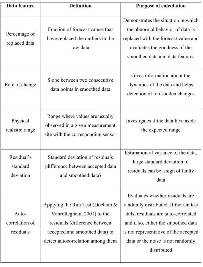
Table 1 – Data features for fault detection ... 44 Table 2 – Model and window size selection, ranked according to the RMSE order ... 65 Table 3 – Exponential smoothing models compared to ARIMA10[2,2] and ARIMA30[1,1] – Accuracy of the 1 step-ahead forecasts ... 69 Table 4 – Fault detection for calibration data set ... 78 Table 5 – Fault detection for validation data sets ... 84

(10)

(11)

xi

List of figures

Figure 1 – The monEAU network concept ... 11

Figure 2 – The monEAU monitoring station installed at the inlet of the primary clarifier at the Lynette wastewater treatment plant in Denmark ... 12

Figure 3 – The equipment panel of the monEAU monitoring station ... 12

Figure 4 – Three steps of the univariate method proposed by Alferes et al. (2012) ... 18

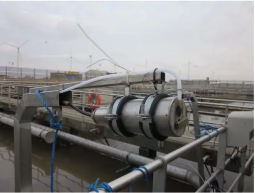
Figure 5 – The case study turbidity sensor installed at the primary clarifier of the Lynette wastewater treatment plant in Denmark ... 33

Figure 6 – The case study turbidity sensor – Sensor fouling problems ... 33

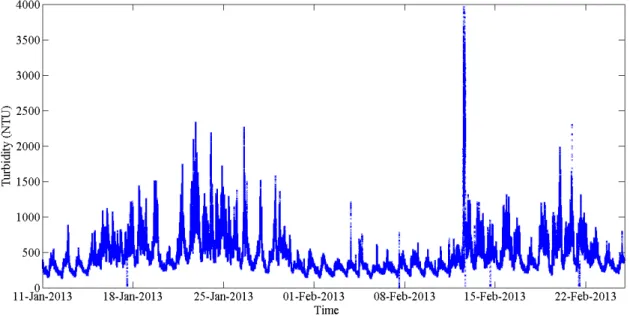
Figure 7 – Raw data – Turbidity – Ts = 5s ... 34

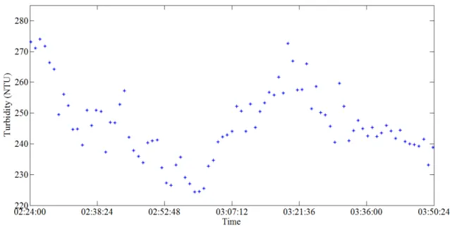
Figure 8 – Turbidity – Ts = 5s – A closer look ... 34

Figure 9 – Re-sampled turbidity – Ts = 1min – A closer look ... 35

Figure 10 – Rainfall intensity data ... 36

Figure 11 – Turbidity – Harmonics ... 36

Figure 12 – Univariate method proposed by Alferes et al. (2012) ... 37

Figure 13 – Graphical representation of the outlier detection algorithm ... 41

Figure 14 – 1st_{order exponential smoothing – Forecasting ... 48}

Figure 15 – 2nd_{order exponential smoothing – Forecasting ... 49}

Figure 16 – 3rd_{order exponential smoothing – Forecasting ... 52}

Figure 17 – Forecasting behavior for a = 0 ... 59

Figure 18 – Forecasting behavior for a = 0.5 ... 60

Figure 19 – Forecasting behavior for a = 1 ... 60

Figure 20 – Moving Window approach ... 61

Figure 21 – Good data for model selection ... 64

Figure 22 – Forecasts with ARIMA30[1,1] ... 66

Figure 23 – RMSE minimization with the 1st_{order exponential smoothing model ... 68}

Figure 24 – RMSE minimization with the 2nd_{order exponential smoothing model ... 68}

Figure 25 – RMSE minimization with the 3rd_{order exponential smoothing model ... 69}

Figure 26 – Application of the moving window ARIMA model to the Univariate method ... 71

Figure 27 – minimization ... 72

Figure 28 – Outlier detection with ARIMA10[2,2] – L = 3 – Bad tuning effects ... 73

Figure 29 – Outlier detection with ARIMA10[2,2] – L = 5 – Good tuning ... 73

(12)

xii

Figure 31 – Univariate method with the ARIMA10[2,2] model – Calibration data set (explanation of the figure, see text) ... 76 Figure 32 – Univariate method with the ARIMA30[1,1] model – Calibration data set (explanation of the figure, see text) ... 76 Figure 33 – Univariate method with the 3rd_{order exponential smoothing model – Calibration data set}

(explanation of the figure, see text) ... 77 Figure 34 – Univariate method with ARIMA10[2,2] model – Validation data set of January 30th

(explanation of the figure, see text) ... 79 Figure 35 – Univariate method with the ARIMA10[2,2] model – Validation data set of April 26th

(explanation of the figure, see text) ... 79 Figure 36 – Univariate method with the ARIMA30[1,1] model – Validation data set of January 30th

(explanation of the figure, see text) ... 80 Figure 37 – Univariate method with the ARIMA30[1,1] model – Validation data set of April 26th

(explanation of the figure, see text) ... 81 Figure 38 – Closer look of the outlier detection of the period marked in Figure 36 (explanation of the figure, see text) ... 82 Figure 39 – Closer look of the outlier detection of the period marked in Figure 37 (explanation of the figure, see text) ... 82 Figure 40 – Univariate method with the 3rd_{order exponential smoothing model – Validation data set}

of January 30th_{(explanation of the figure, see text) ... 83}

Figure 41 – Univariate method with the 3rd_{order exponential smoothing model – Validation data set}

(13)

xiii

Acronyms

AEM : Abnormal Event Management ARMA : Auto-Regressive Moving-Average

ARIMA : Auto-Regressive Integrated Moving Average KF : Kalman filter

MAD : Mean Absolute Deviation

MMFA : Multi Model Filtering Algorithm NTU : Nephelometric Turbidity Unit PC : Principal Component

PCA : Principal Component Analysis RMSE : Root Mean Square Error

VARMA: Vector Auto-Regressive Moving Average WS : Window Size

(14)

(15)

xv

Acknowledgment

I would like to express my deepest gratitude, admiration and respect to my supervisors André Desbiens and Peter A. Vanrolleghem for their unwavering dedication, helpful advices and ongoing supports during my M.Sc. and this research work. I have learned a lot from them and without their helps this work would have never been completed.

I would like to extend my gratitude to Janelcy Alferes Castano for her technical supports and advices. I always felt comfortable to discuss my problems with her and she never hesitated to help me in spite of her occupations.

I also wish to express my thanks to my colleagues and friends in modelEAU with whom I had the precious educational and social experiences.

Many thanks to my friends with whom I have shared many memorable moments during this challenging experience.

I cannot express my loving thanks to my dearest friend and husband, Mohammad who has never stopped believing in me. He has always reminded me of my capabilities and capacities when I was filled with stress, despair and gloom. We have passed many happy and sad moments together in our challenging life in Canada and during all these times he was kindly by my side. Without his supports and understanding, I wouldn’t have finished this work.

Last, but not least, I will thank my parents. In spite of being thousand miles away from me, they have always been the source of my energy. All my exhaustions and frustrations have been vanishing away as I heard their kind voices. They have always admired me because of just being me! Thanks for being my parents, I love you so much!

(16)

(17)

1

1. Introduction

Fault detection and diagnosis which can be regarded as a part of the topic Data Quality Evaluation, has been an important problem in different industries. In the petrochemical industry, for instance, the Abnormal Event Management (AEM) problem was rated as the number one problem to be solved (Venkatasubramanian et al., 2003a). Data quality evaluation is a subject associated to all domains where sensors monitor the state of a system. Thus a variety of mechanisms and techniques have been developed to evaluate the quality of data obtained from application fields as different as nuclear power engineering, chemical engineering, air pollution control, medicine, water supply and distribution networks (Conejo et al., 2007).

Particularly in water systems effective management of water networks and their applications, such as waste water treatment systems and water pollution control, requires reliable information about water quality parameters. Control and modeling of water systems and subsequently making decisions about their performance and judgment about their variations can be carried out with more confidence if the acquired information is reliable. Especially the early diagnosis of process and sensor faults in the systems is of great importance since it facilitates a more precise understanding of the system and more trustable decisions can be made to control, model and supervise the system. Therefore, the reliability of data shall be evaluated attentively and in case of detecting faults, the quality of data shall be improved.

Implementation of automated water quality monitoring stations together with in situ continuous measurement devices measuring with high frequency has been a great step forward in obtaining a better description of water systems. The fast sampling rate enabled by these stations, helps getting along with fast dynamics of water systems and also improving the reliability of the data describing water quality parameters. In other words, the main purpose of implementing automated online water quality measuring stations is to monitor water bodies efficiently and to have a more advanced description of the system’s fast dynamics.

(18)

2

However, the high sampling intensity enabled by online water quality measurement stations leads to collection of huge data sets consisting of a large number of physical-chemical parameters (Alferes et al., 2013b). However, because of the challenges in measuring conditions and sensors, especially during rain events, data collected by means of automated water quality measurement stations are prone to different sources of errors and faults (Rieger & Vanrolleghem, 2008; Hill & Minsker, 2010). In addition, due to the intrinsic properties of water systems, the data sets which describe water quality parameters are often co-linear or auto correlated and not normally distributed (Alferes et al., 2012). Thus, the main objective of implementing the automated water quality monitoring stations will not be efficiently attainable unless the quality of acquired data is verified.

Quality of data registered with automated water quality measurement stations can be largely affected by the conditions of the installed hardware in the field. Some procedures can be followed to improve the quality of acquired data. Regular manual cleaning of the measurement sensors, application of innovative measuring devices with self-cleaning system (Mourad & Bertrand-Krajewski, 2002), increasing the number of measurement sensors and selecting the measurement locations which meet certain criteria (Campisano et al., 2013) are examples of procedures that are followed in the field. However, despite taking all mentioned procedures, the reliability of sensors still remains insufficient and different types of faults in the data are inevitable.

To detect faults in practical systems, outliers in the data should be detected and removed before, since they can negatively affect the performance of the fault detection algorithms. Outliers are known as sample values that behave significantly different from the data points which are believed to depict normal behavior. Outliers might be generated due to different reasons. Sensor noise, temporary sensor failures and human-related errors are examples of sources that contaminate the data with outliers (Liu et al., 2004; Ting et al., 2007). Existence of outliers change considerably different features of the data like mean and variance and also might have negative impact over our interpretation from the system. Therefore, they must be detected, omitted or replaced by more reliable values (Alferes et al., 2012). In automated water quality measurement stations with high frequency which

(19)

3

lead to very large data sets, visual detection of outliers is not feasible thus the need for automated outlier detection methods is motivated (Pearson, 2002).

Peter Vanrolleghem and his research team (modelEAU, Université Laval, Québec, Canada) have developed automated water quality monitoring stations, called monEAUs, with collaboration of public organizations and private companies from North America and Europe (Rieger & Vanrolleghem, 2008). These stations, now available from Primodal Inc. RSM-30, can automatically register different water quality parameters with fast sampling rates in various measurement locations such as rivers, waste water treatment systems and sewers. They comprise sensors for conventional and physical-chemical parameters (temperature, dissolved oxygen, …) as well as innovative sensors like a UV spectrometer and an ion selective device together with water level measurement sensors (Rieger & Vanrolleghem, 2008). Univariate and multivariate methods to detect and replace outlier and to diagnose probable faults in real time have already been developed for these monitoring stations and practically tested successfully by Alferes et al. (2012; 2013b).

The univariate method proposed by Alferes et al. (2012) consists of three successive steps: outlier detection, data smoothing and fault detection. The first and the most challenging step is the outlier detection. This applied method is based on fitting an exponential smoothing model to the data and defining the smoothing model parameters according to historical data. The fitted model is then projected into the future to calculate a one step-ahead forecast value together with its prediction error interval. The prediction error interval is calculated by estimation of the standard deviation of the forecast error. The forecast value plus/minus a multiple of the standard deviation of the forecast error will be considered as the prediction error interval. If the real observed value falls outside this interval, it is considered an outlier and it is replaced by the forecast value.

This research project focuses on the outlier detection step of the previously proposed univariate method. The objective is to propose an alternative method to identify a model for the water quality parameters time series according to which the forecast data will be calculated. The idea is to find a model which results in a better fit to the system and a better forecast of the future behavior of the system in comparison with the exponential smoothing model, in particular with respect to the Root Mean Square Error (RMSE) criterion. The

(20)

4

outliers will then be identified automatically and replaced by the forecast value according to the same approach taken in the previously proposed univariate method. Performance of the new model in detecting outliers will be evaluated in comparison with the exponential smoothing model with respect to a particular set of criteria. In order to achieve this objective, the structure of the work presented in this thesis is as follows:

In the Introduction, the advantage of using automated water quality monitoring stations was discussed. The chapter contained an overview of the general properties of the data series obtained from automated water quality monitoring stations and the necessity of data quality evaluation in such systems.

In chapter 2, Literature Review, first a general introduction of fault detection methods found in literature will be presented ranging from laborious manual techniques to more sophisticated automatic methods. Then the water quality monitoring stations will be introduced and the measurement challenges which lead to the collection of datasets with specific properties will be discussed. Different data quality evaluation approaches found in literature will be presented and feasibility of their application to the case study system will be studied. The exponential smoothing models and their corresponding forecasting equations will be presented for the approach proposed by Alferes et al. (2012), to cope with challenging conditions of monitoring water quality parameters.

Chapter 3, Materials and Methods, begins with the presentation of the case study water quality monitoring stations whose measured water quality parameters will be used to evaluate the performance of the alternative model. The chapter continues with introducing the three steps of the univariate data quality evaluation method proposed by Alferes et al. (2012) and ends with a short discussion about the performance of the method.

Chapter 4, Results, principally includes a mathematical presentation of the alternative model for the system and the method followed to detect outliers in time series data. It also consists of a subchapter which revisits the exponential smoothing model used by Alferes et al. (2012) and discusses the advantage of using an alternative model to forecast the future behavior of the system. The chapter ends with a comparison of the new model and the

(21)

5

exponential smoothing model, regarding outlier detection and data quality evaluation performance.

Chapter 5 draws the conclusions of this work and the suggestions for possible future research plans.

(22)

(23)

7

2. Literature Review

A large number of data quality evaluation methods are proposed in literature ranging from simple visual pre-validation tools to more sophisticated analytical methods, artificial intelligence tools and statistical approaches. Some data quality evaluation methods can be widely applied to several areas while application of some methods is limited due to the assumptions made about their characteristics which make them incompatible to specific procedures. For example when applying a classical Kalman filter (KF), a linear model, quadratic performance criterion and Gaussian probability distribution for the observation noise are assumed (Gandhi & Mili, 2010). However, the performance of KF may degrade significantly in the presence of outliers or, in general, when the state or measurement noise is non-Gaussian (Chan et al., 2005; Ting et al., 2007). Automated water quality monitoring systems have specific characteristics that distinguish them from other systems and limit application of many of data quality evaluation approaches.

In this chapter, first a general introduction of the available approaches in literature will be presented. Subsequently, challenges of water quality monitoring will be discussed and application of the different methods will be practically validated considering the specific conditions of the case study system. An approach to model water quality parameters time series proposed by Alferes et al. (2012) will be discussed and mathematical details will be presented.

2.1. Introduction to data quality evaluation methods

In this section, different types of approaches will be presented and the way they regard the data quality evaluation problem will be discussed.

A very primary classification of the methods comprises off-line and on-line methods or according to another categorization, manual and automatic methods. Off-line data quality evaluation methods such as application of control charts when a reference measurement is available (Thomann et al., 2002) are too tedious and time consuming when huge volumes

(24)

8

of data are registered in on-line automated systems. Application of manual methods, on the other hand, is not feasible in such systems since it requires a full-time inspection operation which is not cost effective (Hill & Minsker, 2010). Accordingly, in automated on-line systems, a serious need for automatic on-line data quality evaluation tools is identified. Automatic on-line data quality evaluation methods can be regarded as univariate or multivariate approaches according to Alferes et al. (2012). In univariate methods the information from single variables are extracted. Multivariate methods detect correlations in the high dimensional measurement space according to which useful information about the measurements is extracted. For a huge amount of correlated data an appropriate method to draw useful information from the data is needed (Aguadoa & Rosen, 2008). For instance in water quality measurement stations, multivariate methods can be used to infer significant information from highly correlated variables. Since univariate methods cannot handle correlation among variables, they can be only applied to evaluate the quality of single water quality parameters. A more reliable decision can be made about the performance of the measurement system if the evaluation result of any single variable done by an univariate method is regarded with respect to other variables.

Another fundamental classification of methods in literature concerns parametric (statistical) methods and non-parametric (model-free) methods. Statistical parametric methods either assume a known underlying distribution of the observations or, at least, they are based on statistical estimates of unknown distribution parameters (Ben-Gal, 2005). These methods are often unsuitable for high-dimensional data sets and for arbitrary data sets without prior knowledge of the underlying data distribution (Ben-Gal, 2005). Within the class of non-parametric approaches, a special categorization can be done for the data-mining methods, also called distance-based methods. These approaches are usually based on local distance measures and are capable of handling large databases (Ben-Gal, 2005). Another category of non-parametric methods consists of the clustering techniques. In these techniques, each object is assigned to the cluster of its nearest neighbor within a certain distance (Abu-el-zeet et al., 2002).

According to Venkatasubramanian et al. (2003a; 2003b; 2003c), fault detection strategies are largely influenced by the type of a priori knowledge which is available about the

(25)

9

system. The a priori knowledge can be developed from a fundamental understanding of the physics of the process expressed in terms of functional relationships between the inputs and outputs of the system which is referred to as, model-based knowledge. On the other hand, the a priori knowledge can be based on the past experience with the process and the availability of a large amount of historical data while it does not assume any form of model information.

Consequently, according to Venkatasubramanian et al. (2003c), from a modeling perspective, fault detection methods can be classified as model-based and process history-based approaches. The model-history-based methods can be subsequently categorized as quantitative or qualitative. In quantitative model-based methods, the a priori knowledge about the process is expressed in terms of mathematical functional relationship between inputs and outputs of the system while in qualitative model-based method this understanding is represented in terms of qualitative functions centered around different units in the process.

There are different ways in which the process history knowledge can contribute as a priori knowledge to the fault detection system. This is known as feature extraction from process history data. Again, one can classify the feature extraction process as either quantitative or qualitative. Quantitative feature extraction can be performed by either statistical or non-statistical methods.

It should be noted that Venkatasubramanian et al. (2003a) give a classification of quantitative model, qualitative model and process history based methods in terms of the intrinsic way these methods approach the problem of fault detection. For instance, KFs (classified under the quantitative model-based methods), which are based on state-space models, broadly use quantitative approaches for generating fault detection results. Similarly neural network methods which basically approach the problem of fault detection from a pattern recognition point of view and hence are classified as process history based methods intrinsically use state-space models (Venkatasubramanian et al., 2003a). If such an overlap of method classifications is accepted, this classification of methods is comprehensive.

(26)

10

By presenting a general introduction of data quality evaluation methods we can have a better perspective on the existing approaches and the feasibility of their application to the case study system. In next section, first the general information about the water quality monitoring stations will be presented. Then the challenging conditions of monitoring of water quality parameters which lead to specific properties of data series will be discussed. Subsequently, different fault detection methods will be presented and the efficiency of their application to the system will be discussed.

2.2. Water quality monitoring challenges and alternatives

2.2.1. The monEAU water quality monitoring stations

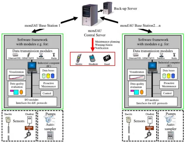
According the monEAU vision for water quality monitoring presented by Rieger and Vanrolleghem (2008), the concept of the resulting monEAU water quality monitoring stations is demonstrated in Figure 1. This figure shows the different components of the monitoring network. It includes the measurement sensors, the monitoring stations and a central server. The monEAU monitoring stations consist of the input/output modules, the industrial computer and the data transmission modules. The sensors measure the water quality parameters and transmit the data to the monitoring stations. The data can be registered in the stations for different monitoring purposes or data quality evaluation or can be transmitted to the central servers for further monitoring and control purposes. The communication protocol between the sensors and the base stations can be quite diverse, but preference is given to bus protocols like Profibus. To connect the monitoring stations to the central server, different telemetry modules are available such as telephone line, xDSL, dedicated radio link and satellite. The monitoring stations are designed to be flexible to be used at different locations such as rivers, WWTPs and sewers with a wide range of types of sensors and sampling methods and with a large set of standard communication protocols for sensor connections. The number of measured variables used so far with these stations can be between 3 and 10 and the sampling time, , can be 5 seconds or 1 minute. Figure 2 shows a typical monitoring station installed in the field, in this case at the inlet of the

(27)

11

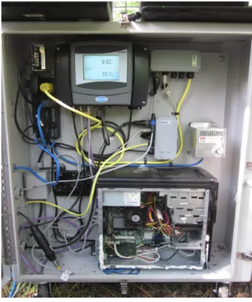
primary clarifier of the Lynette wastewater treatment plant in Denmark. Figure 3 shows the equipments panel of the monEAU station.

(28)

12

Figure 2 – The monEAU monitoring station installed at the inlet of the primary clarifier at the Lynette wastewater treatment plant in Denmark

(29)

13

2.2.2. Characteristics of the water quality monitoring system

As discussed in chapter 1 the high sampling intensity enabled by online water quality monitoring stations leads to collection of huge data sets consisting of a large number of physical-chemical parameters (Alferes et al., 2013b). However, since the measurements are carried out in very difficult and challenging conditions, especially during rain events, data collected from such systems is frequently affected by different types of faults like shift, drift, inaccuracy and sometimes complete failure of the measurement system (Alferes et al., 2013a). In addition, due to the intrinsic properties of water systems, the data sets which describe water quality parameters are often auto-correlated, not normally distributed and noisy (Alferes et al., 2012). Consequently, finding a fault detection approach which is compatible with the operating conditions of this stochastic system with fast dynamics is challenging.

2.2.3. Methods in literature and their applicability in the system

There is an abundance of methods in literature covering model-based and process history-based methods (Venkatasubramanian et al., 2003a) ranging from simple pre-validation tests (Bertrand-Krajewski et al., 2000; Mourad & Bertrand-Krajewski, 2002) to more sophisticated statistical univariate or multivariate tests, model-based and data mining methods (Branisavljevic et al., 2011). Due to the specific characteristics of the case study system, application of a large number of data quality evaluation methods in practice might not be feasible. Model-based methods for instance, need an explicit model of the system to generate residuals (the difference between the actual and expected behavior according to the model) and evaluate them statistically for fault detection purposes (Venkatasubramanian et al., 2003a). However, finding an exact model that explains all physical and chemical variations that might occur especially in this system is a difficult task (Alferes et al., 2013a). On the other hand, process history-based methods can be employed to extract the relationship between input and output of the system according to the history of data without having an accurate model of the system (Venkatasubramanian et al., 2003c; Alferes et al., 2013a).

(30)

14

Automated water quality measurement stations need automatic methods for their quality assurance. As mentioned before, the off-line manual methods are not appropriate for this system. Application of semi-automated data quality evaluation tools in water quality monitoring systems also result in a relatively large percentage of data loss (5-40%) (Bijnen & Korving, 2008; Thomann, 2008). This can be caused by either the inefficiency of the practical methods or by the intrinsic invalidity of data in such systems. On the other hand, on-line application of data quality evaluation approaches is limited to the methods which are not computationally complicated.

Statistical methods have been broadly addressed in literatures as powerful techniques in fault detection in different fields (Willsky, 1976; Basseville, 1988; Conejo et al., 2007; Patcha & Park, 2007); however to apply them safely, accurate information about the system characteristics needs to be available (Conejo et al., 2007). Due to the intrinsic properties of the system, application of pure statistical methods (such as statistical classifiers) might not be feasible since not all behaviors of the system can be expressed as exact statistical distributions (Patcha & Park, 2007).

Patcha and Park (2007) discussed the application of machine learning techniques in the domain of fault detection. They are capable of changing their execution strategies and improve their performance based on previous information. Despite the variety of machine learning approaches available in this domain, these techniques have drawbacks that make them inappropriate for real-time fault detection (Hill & Minsker, 2010). The major problem with many of the machine learning techniques is that they are computationally complex for large volumes of data as collected by automated water quality measurement stations (Patcha & Park, 2007). However, as proposed by Patcha, the idea of the Sliding Window approach in the frame of machine learning techniques can be inspiring to find a way to get adapted to the varying dynamics in the case study system. The idea of using a moving-window approach has also been proposed by Liu et al. (2004) to capture the dynamic variations in on-line process data for outlier detection purposes.

As previously discussed in 2.1, according to the process history-based model categorization (Venkatasubramanian et al., 2003c), there are feature extraction methods that present the historical process data as a priori knowledge to the fault detection system. This is also

(31)

15

known as data-mining in the literature. It is the process of extracting patterns from the data to allow later diagnosis according to the deviation of future behavior with the historical pattern (Patcha & Park, 2007; Hill & Minsker, 2010). For stochastic systems, like the water quality monitoring stations, whose future state is not completely determined by the past and present status of the system, statistical feature extraction methods can be useful too.

The previously discussed idea of generating residuals is also known as analytical redundancy in literature (Basseville, 1988; Bloch et al., 1995; Hill & Minsker, 2010). In this approach the output of a model which is fitted to the data stream is considered as a redundant sensor whose measurement can be compared with that of the actual sensor. Classification of a data point as anomalous or non anomalous is performed according to the difference between model prediction and sensor measurement considering a threshold value (Pastres et al., 2003; Garcia et al., 2010; Hill & Minsker, 2010; Alferes et al., 2012). Since faults in the system cause changes in state variables or model parameters, analytical redundancy for fault detection in dynamic systems, mostly concerns monitoring of estimated states or model parameters of the system (Venkatasubramanian et al., 2003a). According to the solution given by Willksy (1976), Basseville (1988) discussed the application of KFs to give optimal state estimates according to the model of the system. KF is a well known model-based tool that uses underlying dynamic models to estimate the current state of process variables given the noisy measurement data (Bai et al., 2006). The filter can also estimate the corresponding output data by using the estimates of the states of the dynamic system (Ting et al., 2007).

However, as mentioned at the beginning of chapter 2, some assumptions are made in the application of the classical KFs that may degrade their efficiency (Chan et al., 2005; Ting et al., 2007; Gandhi & Mili, 2010). To address this problem, different solutions have been presented in literature comprising consideration of non-Gaussian distributions for random variables (West, 1981; Smith & West, 1983) or addressing the sensitivity of the squared error criterion to noises (Huber, 1964). To get along with the nonlinearity of systems, Extended KFs can be used to estimate the states of the system by a nonlinear state space model of the system (Basseville, 1988).

(32)

16

Application of KFs to water quality monitoring stations can be challenging because of the specific properties of these systems. The mentioned robustification approaches can be numerically complicated and thus might not be applicable to the case study water system. In addition, due to the existence of unknown disturbances in this system, the stochastic behavior of the monitored water quality parameters can hardly be precisely known and thus, one single model cannot describe the behavior of the system. A possible solution can be adopting the system model by using the Extended KFs. Another possible approach is the application of a bank of KFs, working independently, designed for all possible modes of behavior in the system (Basseville, 1988; Maldonado et al., 2010).

Maldonado et al. (2010) presented the Multi Model Filtering Algorithm (MMFA). In their method, at the calibration phase that uses the history of data, a set of linear models is identified for different behavioral modes of the system. For each of the identified models a KF is designed according to which the states of the system are estimated. To improve state estimation by applying Bayes’ rule the conditional probability of each model to represent the actual observed system behavior based on input and output measurements is determined. The final estimated state of the system is calculated as a weighted sum of model probabilities and their associated states. In water quality monitoring systems, it is hard to find the optimal number of possible models of the system; therefore the size of bank of KFs may increase (Venkatasubramanian et al., 2003a). This is the reason that the application of this approach in this system may not be as straightforward as it seems. Auto-Regressive data-driven methods are a class of data quality evaluation approaches that are widely used in literature. They are known to be successful in empirical modeling of time series data. Hipel and McLeod (1978) demonstrate that data-driven Auto-Regressive Moving-Average (ARMA) models can be successful in modeling hydrological time series data. According to them, the stochastic model is fitted to the system empirically and it does not exactly represent the physical model of the system. Similarly, Berthouex and Box (1996) state that an Auto-Regressive Integrated Moving Average (ARIMA) model can be fitted empirically to the stochastic time series obtained from waste water treatment plant to auto-forecast (uses just its own past to forecast future) future values of the series. Although the obtained model is identified empirically and does not exactly represent all

(33)

physical-17

chemical phenomena, it can be interpreted as a faithful description of physical-chemical realities. Garcia et al. (2010) also use a Vector Auto-Regressive Moving Average (VARMA) model (which is the extension of ARIMA model to the multivariate case) to predict and detect failures in railway networks. They identify parameters of the model using the Maximum Likelihood approach.

2.2.4. The alternative approach

Considering the intrinsic characteristics of the automated water quality measurement systems, it can be concluded that the alternative method should be automatic to scale well with the large volume of data, on-line applicable in real-time and fast enough to get along with the rate of data collection. In addition, it should not be computationally complicated and should not need any form of model as a priori knowledge. Since finding a physics-based model is hard while a large volume of data history is available, a data-driven time series model can be used (Hill & Minsker, 2010). Consequently, it is proposed to use the ARMA model as an alternative to the expected characteristics. The model can be identified according to the history of the data and the expected behavior in the future can be forecasted based on the identified model. To adapt to the varying dynamics, the moving window idea can be employed and to detect outliers, according to the analytical redundancy concept, deviation of the expected behavior from the real behavior can be identified.

2.2.5. Methods proposed by Alferes et al. (2012)

Regarding the utilization of data-driven models, Alferes et al. (2012) discussed two different approaches to assess data quality in automated water quality monitoring stations according to the history of data without having a theoretical model of the system. One is the univariate method which employs time series data of a single variable to check the acceptability of the measurement noise (Campisano et al., 2013) by means of autoregressive models. The other one is the multivariate method which infers significant

(34)

18

information from highly correlated variables based on Principal Component Analysis (PCA) (Yoo et al., 2008).

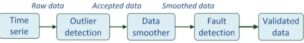
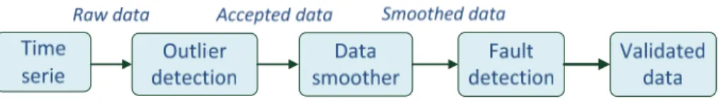
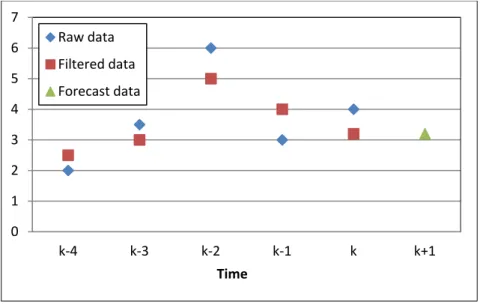
The univariate method comprises three consecutive steps (Figure 4). The first and the most challenging step is the outlier detection. According to this approach, a 3rd_{order exponential}

smoothing model is fitted to the time series data and its parameters are estimated. The model is then projected into the future to generate the one-step ahead forecast data. The standard deviation of the forecast error (the difference between the forecast and observed values) is predicted at each time step by means of the 1st_{order exponential smoothing}

model. The prediction interval is defined by adding or subtracting a multiple of the standard deviation of forecast error to the forecast value. If the observed value at each time step falls out of the prediction interval, it will be regarded as an outlier. Once an outlier is detected, it is replaced by the forecast value. The output of this step is called the “Accepted data” which is smoothed in the next step of the method, using a kernel smoother to remove noise. Potential sensor faults are then identified in the third step by applying acceptability limits to the data features extracted from the filtered data calculated in the previous step.

Figure 4 – Three steps of the univariate method proposed by Alferes et al. (2012)

Since water quality data are highly auto and cross-correlated and univariate methods cannot intrinsically handle correlation among variables, Alferes et al. (2012) propose a multivariate method to infer significant information from highly correlated variables. The multivariate method is based on Principal Component Analysis (Yoo et al., 2008). In the PCA method, a new set of uncorrelated and orthogonal variables, called Principal Components (PCs), are extracted. Each PC is a linear combination of original variables which describe the largest process variability in a space with fewer dimensions than the original one. In order to detect probable faults in the multivariate method, it is proposed to calculate two statistics, T2 and Q, which describe the fit of the model to the system.

(35)

19

Comparison of the calculated statistics with their correspondent confidence intervals, leads to detection of probable faults in the original system.

The univariate and multivariate methods developed by Alferes et al. (2012) have been successfully applied to detect and replace doubtful data and to diagnose probable faults in real time data series collected by the automated monitoring stations in modelEAU. In this research project, the univariate method is regarded with special attention. The outlier detection step will be studied in more details and its efficiency will be commented. The objective is to provide improvements to the univariate method regarding the model fitted to the system and the way the one-step ahead forecasts are generated.

2.3. The objective of the project

As mentioned before, the objective of this research project is to improve the univariate data quality evaluation method of Alferes et al. (2012) that detects outliers and probable faults in water quality parameters measured by the automated water quality monitoring stations. The evaluation method consists of three consecutive steps and the focus of this work will be on the first step which is where outliers are detected. To detect outliers in the univariate method, a 3rd_{order exponential smoothing model is fitted to the time series data and is used}

to perform a one-step ahead forecast. In this work the exponential smoothing models will be critically evaluated and the manner in which they fit to the data series and forecast one-step ahead will be discussed. Subsequently, another forecasting model will be suggested to replace the 3rd_{order exponential smoothing model to give one-step ahead forecasts. As for}

the exponential model this alternative model must be accompanied with an approach to adapt the model to the varying dynamics in the data. The proposed forecasting approach will be applied to a case study water quality parameter and the accuracy of the one-step ahead forecasts will be compared to the ones obtained by the 3rd order exponential smoothing model. Both forecasting models will finally be compared through their performance within the univariate data quality evaluation method. Their efficiency will be compared in terms of detecting probable faults in the case study time series according the specified criteria.

(36)

20

2.4. Exponential smoothing models in forecasting time series

The performance of the outlier detection step in the univariate method is principally based on forecasting time series data according to the historical behavior by means of exponential smoothing models. Therefore, in this section more details are presented about these models and the way they generate forecasts.

As mentioned by Montgomery et al. (1990), exponential smoothing is a popular method for smoothing discrete time series in order to forecast immediate future. Exponential smoothing models use special weighted moving averages and a seasonal factor that is multiplied by the weighted moving average in order to forecast the immediate future. These weighted moving averages are referred to as smoothing statistics. The exponential smoothing models are an extension of the moving average model. Generally, an exponential smoothing method uses three smoothed statistics that are weighted, so that the more recent the data, the more weight is given to the data in producing the forecast. These three averages are referred to as single, double, and triple smoothing statistics and are moving averages that are weighted in an exponential declining way.

According to Montgomery et al. (1990), forecasting systems use three separate forecasting equations: one model called a constant model, the second called a linear model and a third called a quadratic model. The constant forecast uses only the single smoothed statistic and performs well when the time series has little trend. The linear forecast model uses the single and double smoothed statistics and is good when there is a linear trend in the time series. The quadratic forecast model uses all three statistics namely, single, double, and triple smoothed statistics.

In the next section, different orders of exponential smoothing models will be discussed. It includes details about the models, estimation of their unknown parameters and the way they produce forecasts for the future according to Montgomery et al. (1990). Since the objective is to improve the quality of the model in generating more accurate forecasts, a mathematical revision of the models is essential. An alternative model can then be proposed once all the details are understood about the current model.

(37)

21

2.4.1. Simple exponential smoothing for a constant process

If one could assume that the average of a time series does not change over time or if it does, it changes very slowly, the fitted discrete-time model might take the form:

k k

x b

 



(1)

where represents a discrete time sample, is the data value at time , is the mean value of the data set and the model’s unknown parameter and denotes a random error term corresponding to that part of the data that cannot be fitted by the model. The random term in the model is considered to have an expected value of zero and the constant variance.

At the end of time step , a data history , , … , is available according to which we wish to estimate the unknown model parameter . To do so, the simple (first) exponential smoothing model can be used.

In this forecasting system, the model parameters are re-estimated at each time . In order to take into account the data observed in the most recent period, it can be assumed that at the end of period we have available the estimate of made at previous time 1, i.e. and the actual value of current time , to calculate an updated estimate . A reasonable way to get the updated estimate is to modify the old estimate with a fraction of the forecast error. The forecast error at time , results from the difference between the current observed value and the old estimate.

1

ˆ

k k k

e  x b  (2)

The new estimate is computed according to the following equation:

1 1

ˆ ˆ _[ ˆ _]

k k k k

b b _  x b _ (3)

, namely the smoothing constant, is the fraction according to which we desire to contribute the forecast error to the calculation of the new estimate.

(38)

22

For simplification of the further development of the methods, we define the first exponentially smoothed statistic as ≡ . So the above equation will be:

1 [ 1] k k k k s s_ 



x s _ (4) In other words:



1 

1 k k k

s





x

 



s

_ (5)

The presented procedure is called Simple (First) Exponential Smoothing.

Generally speaking, the smoothed statistic constitutes a weighted average of past observations where the weights sum to unity and decrease geometrically with the age of the observations. These statements can be proven if in the right-hand side of equation (5) is substituted recursively by its equivalent from equation (5). This operation leads to the following equation: 1 0 0 (1 ) (1 ) k m k k k m m s    x   s  



   ₍₆₎

where is the initial estimate of and is used to initialize the algorithm. The weights add to 1 since:

1 0 1 (1 ) (1 ) 1 (1 ) 1 (1 ) k k m k m                 



(7)

The smoothing constant presented in equation (3) is the forgetting factor in this method which controls the rate of decay and determines the behavior of the forecast system with respect to the changes in . Small values of give more weight to the historical data promoting a slow response. With large values of , more weight is assigned to the current observation while leading to a faster response. Generally, the value can range between 0 and 1, taking typical values between 0.01 and 0.3.

(39)

23

As already mentioned and proven in equation (6), the weights associated to previous observations decay with time and since these weights decrease exponentially with time, the name exponential smoothing is assigned to this procedure.

For a large enough value of , i.e., the term 1 is very close to zero, the exponential smoothing operator described in equation (6) leads to an unbiased estimate of the real value of the process average , since:

0 0 0 ( ) [ (1 )m ] (1 ) (m ) (1 )m k k m k m m m m E s E   x_    E x_ b   b    



 



 



  ₍₈₎

So, it is logical to take as the estimator of the unknown parameter of the model at time :

ˆ_k _k

b s (9)

Finally, because a constant model is considered, the forecast value of the data for any future time steps would be:

ˆ

_{k j} _k

x





b

(10)

To sum up, a first order exponential smoothing operator fits a constant model to the time series data (equation(1)) whose only unknown parameter is re-estimated at each time as the new data point emerges (equations (4) and (9)). Since a constant model is considered, for any time in future the estimated model at current time is projected into future and according to that the forecast of the data is produced (equation (10)).

2.4.2. Double exponential smoothing for a linear trend process

A second order exponential smoothing model is the extension of the first order exponential smoothing to the cases in which the mean of the process changes linearly with time and there is a trend in the data, according to the following discrete-time model:

(40)

24

k k

x

 

a bk





(11)

where the intercept and the slope of the linear model are the unknown parameters which are supposed to be estimated. The definitions of and remain the same as the ones for the constant model in the previous section.

If the simple exponential smoothing operator described in equations (6) is applied to the linear process defined in equation (11) and the expected value is calculated, we obtain:

1 0 0 1 0 0 ( ) ( ) [ ( )] k m k k k m m k m k m E s E x s a b k m s                 



(12)

where is equivalent to 1 and is considered for simplification of the demonstrations. For sufficiently large value of , tends to zero, then equation (12) can be expressed as:

0 0 ( ) ( ) m m k m m E s a bk   b m a bk  b       







   ₍₁₃₎ and since, ( )_k E x  a bk ₍₁₄₎

for equation (13) we have: ( )k ( )k

E s E x



b



  (15)

This means that the expected value of the first order exponentially smoothed statistic, when applied to a linear model, lags behind the process by a value equal to .

(41)

25 [2] [2] 1 (1 ) k k k s 



s  



s _ (16)

where denotes double (second-order) exponential smoothing. Similarly for the output of equation (15) we can show that:

[2] ( )_k ( )_k E s E s b    ₍₁₇₎ And consequently, [2] [ ( )k ( )]k b  E s E s    ₍₁₈₎

So it is reasonable to estimate b at the end of time period as:

[2] ˆ _[ _] k k k b  s s    ₍₁₉₎

By substituting equation (17) in equation (15), the expected value of the data at the end of the time period can be obtained as:

[2] [2] ( ) ( ) [ ( ) ( )] 2 ( ) ( ) k k k k k k E x E s E s E s E s E s           (20) Therefore, it seems reasonable to say:

[2]

ˆk 2 k k

x  s s (21)

On the other hand, estimation of can be performed according to two different approaches which both lead to the same estimation of the intercept. One is to estimate the intercept at the original time origin by employing equations (19) and (21), as:

(42)

26





[2] [2] ˆ ˆ_k ˆ_k _k 2 _k _k _k _k a x kb  s s k



_

s s ₍₂₂₎

According to this approach, the calculation of the forecast value made at time for any time step in the future will be:





ˆ

ˆ_{k j} ˆ_k _k

x  a  k j b (23)

Another approach is to think the origin of time as shifted to the end of time period and then estimate the current-origin intercept according to the following equation:

[2] ˆ ˆ 2 k k k k a x s s    (24)

In this case, the forecasting equation for any time step in future is as follows: ˆ

ˆ_{k j} ˆ_k _k

x  a jb (25)

Initial values of and are obtained from initial estimates of the two coefficients and which may be developed through simple linear regression analysis of historical data.

2.4.3. Triple exponential smoothing for a process with quadratic model

A third order (triple) exponential smoothing model takes into account trends and seasonal changes. The corresponding model takes the quadratic form:

2

1 2

k k

x  a bk ck   ₍₂₆₎

According to the explanations presented in the previous sections, assuming that we have estimates of the model parameters based on the original origin of time, the forecasting equation at the end of period for step ahead is:

(43)

27





ˆ 1 2 ˆ ˆ ( ) ˆ 2 k j k k k x    a k j b  k j c (27)

However, if we define the origin of time at the end of the period , the coefficients will take different values and the forecasting equation will be:

2 1 ˆ ˆ ˆ ˆ 2 k j k k k x  a b j c j (28)

For the latter case, the coefficients of the model, , and ̂ are computed using the first, second and third exponentially smoothed statistics, , and calculated at the end of time period . The smoothed statistics are calculated by:





 

_

_

     

_

_

  1 2 2 1 3 2 3 1 1 1 1 k k k k k k k k k s x s s s s s s s                   (29)

Once the statistics have been calculated, the coefficients of the model are obtained as follow:    













 





     





2 3 2 3 2 2 2 3 ˆ 3 3 ˆ _{6 5} _{2 5 4} _{4 3} 2 1 ˆ 2 1 k k k k k k k k k k k k a s s s b s s s c s s s  _ _ _          _      _    _ _      (30)

Therefore, in the third order exponential smoothing model, a quadratic model (equation (26)) will be considered for the system. The unknown parameters of the model, , and , can be estimated at each time step through equations (30), while the smoothing statistics have been already calculated through equations (29). The forecast for any time step in future can be generated by projecting the quadratic model into the future through equation (27).

(44)

28

2.4.4. Simple exponential smoothing in calculating the Standard Deviation of forecast error

The exponential smoothing models are used in the univariate method to first, produce the one step-ahead forecasts and then to calculate the standard deviation of the forecast error to detect and replace outliers in water quality parameter time series. At each time step, the forecast is calculated together with its prediction error interval which gives the amount by which the real observed data can deviate from the forecast data.

The prediction error interval is indentified by analyzing the one-step-ahead forecast error at each time step, 1 calculated as:

ˆ (1)

k k k

e  x x (31)

where is the forecast for time made at previous time step, 1 and is the real observed value at time .

To provide an estimation of the local variance and to quantify the extent by which the actual value differs from the forecast according to Montgomery (2009), a method is applied to estimate the variance of forecast error, , through the estimation of the Mean Absolute Deviation (MAD), , by means of a simple exponential smoothing model. According to this method, assuming that the forecast error is normally distributed at time , the estimate of is obtained as:

, ˆ

ˆe k 1.25 k



  (32)

where , is the estimate of the standard deviation of forecast error for time and ∆ ,

calculated according to the 1st_{order exponential smoothing method as:}

  



1

ˆ_k _e_k ₁ ₁ ˆ_k_

       ₍₃₃₎

(45)

29

Finally, the prediction error interval, , is defined based on a probability statement about the forecast error by adding or subtracting to the forecast data a multiple of the standard deviation of the forecast error:

,

ˆ ˆ

k k e k

xlim x L 



₍₃₄₎

where is a proportional constant. Smaller values of make the limits more restrictive while larger values lead to less restrictive limits.

In this chapter, the exponential smoothing models used in forecasting the data as well as used for estimation of the prediction error interval, were explained. The next chapter is dedicated to the explanation of the water quality monitoring system and its corresponding measured variables. Details of the three steps of the previously explained univariate data quality evaluation method will then be presented. An alternative method cannot be proposed unless a complete knowledge about the previous method is acquired.

(46)

(47)

31

3. MATERIALS AND METHODS

As discussed in section 2.3, the objective of this project is to propose a new model to fit to the fast dynamics of the time series that describe water quality parameters in the monEAU automated water quality monitoring stations. General information about these stations is presented in section 2.2.1. The monitoring stations have been so far installed in different water sources with diverse purposes. The case study in this project is a station installed at the municipal treatment plant in Denmark. Time series related to one of the water quality parameters in this station will be selected and the new method will be calibrated and its performance will be evaluated according to that.

In this chapter, first the case study monitoring station will be introduced. The water quality parameter registered by this station, which will be used for tuning and evaluation of the new model, will be introduced. The chapter continues with an explanation of the different steps of the previously discussed univariate method. With a focus on the outlier detection step, the chapter ends with a discussion about the potential of substituting the forecasting model of the outlier detection system.

3.1. In situ monitoring station – Case study

As mentioned before, the automated water quality monitoring stations, monEAUs, have been installed in different water systems with different purposes. The case study in this project used two automated monitoring stations (RSM30, Primodal System) which were installed one at the inlet and the other one at the outlet of a primary clarifier of the 700,000 PE municipal treatment plant in Lynetten (Copenhagen, Denmark) (Alferes et al., 2013b). Figure 2, illustrates one of the mentioned monitoring stations. The objective of installing these stations was to study the inflow dynamics as well as the performance of the primary clarifier. To achieve this objective, these stations comprise the following measurement instruments:

Automatic outlier detection in automated water quality measurement stations