Nonlinear bounded-error parameter estimation using interval computation

HAL Id: hal-00845125

https://hal.archives-ouvertes.fr/hal-00845125

HAL is a multi-disciplinary open access archive for the deposit and dissemination of sci-entific research documents, whether they are pub-lished or not. The documents may come from

L’archive ouverte pluridisciplinaire HAL, est destinée au dépôt et à la diffusion de documents scientifiques de niveau recherche, publiés ou non, émanant des établissements d’enseignement et de

Nonlinear bounded-error parameter estimation using

interval computation

Luc Jaulin, Eric Walter

To cite this version:

Luc Jaulin, Eric Walter. Nonlinear bounded-error parameter estimation using interval computation. Witold Pedrycz. Granular Computing: An Emerging Paradigm, Physica Verlag Heidelberg, pp.397, 2001, Studies in Fuzziness and Soft Computing, Vol. 70, 978-3-7908-1387-6. �hal-00845125�

Nonlinear Bounded-Error

Parameter Estimation

Using Interval Computation

L. Jaulin and E. Walter

!"#$!%#&$' (') *&+,!-. '% */)%01')2 345*6*-789':6;,&<'$)&%8 (' =!$&)6*-(2 =9!%'!- (' >#-9#,2 ?@@?A B&C6)-$6D<'%%'2 E$!,:'

F, 9'!<' C$#1 !"#$!%#&$' (GH,+8,&'$&' (') */)%01') I-%#1!%&)8)2 ;,&<'$)&%8 (GI,+'$)2 E!:-9%8 (') *:&',:')2 A "#-9'<!$( !<#&)&'$2 J?KJL I,+'$)2 E$!,:'

Abstract: This paper deals with the estimation of the parameters of a model from experimental data. The aim of the method presented is to characterize the set S of all values of the parameter vector that are acceptable in the sense that all errors between the experimental data and corresponding model outputs lie between known lower and upper bounds. This corresponds to what is known as bounded error estimation, or membership set estimation. Most of the methods available to give guaranteed estimates of S rely on the hypothesis that the model output is linear in its parameters, contrary to the method advocated here, which can deal with nonlinear model. This is made possible by the use of the tools of interval analysis, combined with a branch-and-bound algorithm. The purpose of the present paper is to show that the approach can be cast into the more general framework of granular computing.

1

Introduction

In the exact sciences, in engineering, and increasingly in the human sciences too, math-ematical models are used to describe, understand, predict or control the behavior of systems. These mathematical models often involve unknown parameters that should be identi…ed (or calibrated, or estimated) from experimental data and prior knowledge or hy-potheses (see, e.g., [WP97]). Let y_!; k 2 f1; : : : ; k _!"g; be the data collected on the system to be modeled. They form the data vector y2 R! !"_{. Denote the vector of the unknown}

M(p). For any given p, M(p) generates a vector model output y (p) homogeneous to the data vector y. Estimating p from y is one of the basic tasks of statisticians. This is usually done by minimizing some cost function j(p), for instance a norm of y ¡ y (p). The Euclidean norm is most commonly used, leading to what is known as least-square estimation. It corresponds to maximum-likelihood estimation of p under the hypothesis that the data points y_! ; k 2 f1; : : : ; k _!"g; are independently corrupted by an additive Gaussian measurement noise with zero mean and covariance independent of k. Many other cost functions may be considered, depending on the information available on the noise corrupting the data. The minimization of these cost functions usually lead to a point estimate of p, i.e., a single numerical value for each parameter. Except in a few special cases, the minimization of the cost function is di¢cult and one can seldom guarantee that a global optimizer of the cost function has been found. Moreover, the characterization of the uncertainty on the estimate of p is usually performed, if at all, by using asymptotic properties of maximum-likelihood estimators, which is not appropriate when the number k !" of data points is very small, as is often the case in biology for example. An attractive

alternative is to resort to what is known as bounded-error estimation or set-membership estimation. In this context (see, e.g., [Wal90], [Nor94], [Nor95], [MNPLW96] and the ref-erences therein), a vector p is feasible if and only if all errors e_!(p) between the data points y_! and the corresponding model outputs y _"!(p) lie between known lower bounds e_! and upper bounds ¹e!, which express the con…dence in the corresponding measurement.

Let S be the set of all values of p that are feasible, i.e.,

S_{= fp 2R}# _{j for all k 2 f1; : : : ; k !"g; y!¡ y "!(p) 2 [e!; ¹e!]g (1)}

Some methods only look for a value of p in S, but then the size and shape of S, which provide useful information about the uncertainty on p that results from the uncertainty in the data, remain unknown. This is why one should rather try to characterize S. When y (p) is linear, S is a convex polytope, which can be characterized exactly [WPL89]. In the nonlinear case, the situation is far more complicated if one is looking for a guaran-teed characterization of S. The algorithm sivia (for Set Inverter Via Interval Analysis) [JW93a], [JW93c], [JW93b] nevertheless makes it possible to compute guaranteed esti-mates of S in many situations of practical interest, by combining a branch-and-bound algorithm with techniques of interval computation. The purpose of this chapter is to present the resulting methodology in the framework of granular computing. The chapter

is organized as follows. In Section 2, the very few notions of interval analysis required to understand sivia are recalled. Section 3 presents this algorithm in the context of gran-ular computing. Its application to nonlinear bounded-error estimation is illustrated on a simple example in Section 4.

2

Interval computation

Interval computation was initially developed (see [Moo79]) to quantify the uncertainty of results calculated with a computer using a ‡oating point number representation, by bracketing any real number to be computed between two numbers that could be repre-sented exactly. It has found many others applications, such as global optimization and guaranteed solution of sets of nonlinear equations and/or inequalities [Han92], [HDM97]. Here, we shall only use interval computation to test whether a given box in parameter space is inside or outside S:

An interval [x] = [x; x] is a bounded compact subset of R. The set of all intervals of R will be denoted by IR. A vector interval (or box) [x] of R is the Cartesian product of n intervals. The set of all boxes of R will be denoted by IR . The basic operations on intervals are de…ned as follows

[x] + [y] = [x + y; x + y]; [x] ¡ [y] = [x ¡ y; x ¡ y];

[x] ¤ [y] = [minfxy; xy; xy; xyg; maxfxy; xy; xy; xyg]; 1=[y] = [1=y; 1=y] (provided that 0 =2 [y]);

[x]=[y] = [x] ¤ (1=[y]) (0 =2 [y]):

All continuous basic functions such as sin, cos, exp, sqr... extend easily to intervals by de…ning f ([x]) as ff (x)jx 2 [x]g: As an example, sin ([0; ¼=2]) ¤ [¡1; 3] + [¡1; 3] = [0; 1] ¤ [¡1; 3] + [¡1; 3] = [¡1; 3] + [¡1; 3] = [¡2; 6] : Note that some properties true in R are no longer true in IR. For instance, the property x ¡ x = 0 translates into [x] ¡ [x] 3 0, and the property x = x ¤ x translates into [x] ½ [x] ¤ [x] :

Example 1 If [x] = [¡1; 3] ; [x] ¡ [x] = [¡4; 4], [x] = [0; 9] and [x] ¤ [x] = [¡3; 9].

by the same sequence on intervals containing these real numbers, then the interval result contains the corresponding real result. ¥

Example 2 Since [0; 2]+ ([2; 3] ¤ [4; 5])¡[2; 3] = [0; 2] +[8; 15]¡ [2; 3] = [8; 17]+[¡3; 2] = [5; 19], the result obtained by performing the same computation on real numbers belonging to these intervals is guaranteed to belong to [5; 19]. For instance 1 + (2 ¤ 5) ¡ 2 = 9

2 [5; 19]. ¥

For any function f from R to R which can be evaluated by a succession of elementary operations, it is thus possible to compute an interval that contains the range of f over a box of IR . Depending on the formal expression of the function the interval obtained may di¤er, but it is always guaranteed to contain the actual range. This is illustrated by the following example for n = 1.

Example 3 The function de…ned by f (x) = x ¡ x can equivalently be de…ned by f (x) = (x ¡ 1=2) ¡1=4. The range of f over [x] = [¡1; 3] can thus be evaluated in the two following ways.

[x] ¡ [x] = [¡1; 3] ¡ [¡1; 3] = [0; 9] + [¡3; 1] = [¡3; 10]; ¡[x] ¡ !¢

¡!_" = £¡#;$¤

¡ !_" =£0; $_"¤ ¡ !_" =£¡!_"; 6¤: (2)

The …rst result is a pessimistic approximation of the range, whereas the second one gives the actual range. This is due to the fact that in the …rst expression [x] appears twice, and that the actual value of x in the two occurrences are assumed to vary independently within [x] : It is thus advisable to write the functions in such a way as to minimize the number

of occurrences of each variable. ¥

Let f be a function from R to R and [a; b] an interval. Interval computation will provide su¢cient conditions to guarantee either that

8x 2 [x] 2 IR ; f (x) 2 [a; b]; (3)

or that

Of course, when part of f ([x]) belongs to [a; b] and part does not, no conclusion can be reached using these conditions. Although the number of x in [x] is not even countable, these conditions will be tested in a …nite number of steps. For this purpose, an enclosure [f ] of the range f ([x]) will be computed using interval computation.

² if [f ] ½ [a; b] then all x in [x] satisfy (3),

² if [f ] \ [a; b] = ;, then no x in [x] satis…es (3), or equivalently all of them satisfy (4).

Note that if these two tests take the value false, then no conclusion can be drawn. These basic principles will be used to test whether a given box in parameter space [p] is either inside or outside S, where S is given by (1). It su¢ces to compute an enclosure [e ] of y ¡ y_!" ([p]) for all k 2 f1; : : : ; k _!"g, using interval computation.

² if for all k in f1; : : : ; k _!"g; [e ] ½ [e ; ¹e ], then [p] ½ S.

² if there exists k in f1; : : : ; k _!"g, such that [e ] \ [e ; ¹e ] = ;, then, [p] \ S = ;:

Again, the fact that boxes are considered instead of vectors will allow the exploration of the whole space of interest in a guaranteed way in a …nite number of steps, as opposed to Monte-Carlo methods that only sample a …nite number of points and can thus not guarantee their results. When no conclusion can be reached for the box [p], it may be split into subboxes on which the tests will be reiterated, as in the next section.

3

SIVIA

The principle of the Set Inverter Via Interval Analysis algorithm is to split the initial problem of characterizing S into a sequence of more manageable tasks, each of which is solved using interval computation. sivia thus pertains to the framework of granular computing.

The parameter vector p is assumed to belong to some (possibly very large) search domain [p_#]. Let " be a positive number to be chosen by the user; " will be called the level of

information granularity. A layer associated with S at level " is a list G(") of nonoverlaping colored boxes [p] that cover [p ], where ,

1. [p] is black if it is known that [p] ½ S,

2. [p] is grey if it is known that [p] \ S =;,

3. [p] is white in all other cases.

Note that some white boxes may actually satisfy either [p] ½ S or [p] \ S = ;, because of the pessimism of interval computation. Each box of G(") is called a granule. The knowledge required to color it may have been obtained by using the techniques explained in Section 2. Moreover, all white boxes in G(") are such that their widths are smaller than or equal to ".

The principle of a procedure to build a layer G(" ) associated with the set S is described by the following algorithm. As most granular algorithms, it generates a sequence of layers G_{(") indexed by the level of information granularity " for decreasing values of ". Starting} from a very coarse representation associated with a large " corresponding to the width of the initial search domain, it stops when " becomes smaller than or equal to " . In what follows, w([p]) is the width of [p] ; i.e., the length of its largest side, and splitting a box means cutting it into two subboxes, perpendicularly to its largest side.

!"#" $%&%'# ('") %* $%+'#") (',-.'('/0 !"/ !(1" ,""2 $!%#"2 .% *($-&-.(." .!" 1-#+(&-3(.-%2 %* .!" ,%+24('/ %* 0

Sivia_{(in: [p ]; " ; out: G));}

1 " := w([p ]); Paint [p ] white; G := f[p ]g; 2 while " ¸ " ; do

3 " := "=2;

4 while there exists a white [p] of G such that w([p]) > "; 5 split [p] into [p_!] and [p_"];

6 if attempt to prove that [p_!] ½ S is a success, then paint [p_!] black; 7 if attempt to prove that [p_!] \ S =; is a success, then paint [p_!] grey; 8 otherwise, paint [p_!] white;

9 if attempt to prove that [p_"] ½ S is a success, then paint [p_"] black; 10 if attempt to prove that [p_"] \ S = ; is a success, then paint [p_"] grey; 11 otherwise, paint [p_"] white;

12 endwhile; 13 endwhile; 14 return G.

Denote the union of all black boxes by S and the union of all black and white boxes by S#_{. At each iteration of the external while loop, one then has}

S _{½ S ½ S}#_{: (5)}

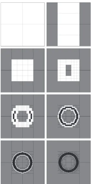
Example 4 Consider the set S described by

S_{= fp 2R}"_jp"_{!+ p}"_{" 2 [1; 2]g:}

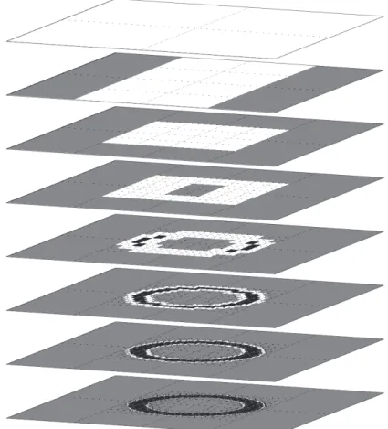
For [p ] = [¡3; 3] £ [¡3; 3] and " = 0:04, sivia generates the sequence of layers described by Figure 1. Each of these layers corresponds to the state of G at Step 13. The hierarchical properties of these layers are schematically portrayed by the information pyramid of Figure 2.

4

Application to bounded-error estimation

Consider a model where the relation between the parameter vector p and the model output is given by

We choose a two-parameter model to facilitate illustration, but note that the method applies to higher dimensions without modi…cation. This speci…c example was chosen to show that the methodology advocated in this paper was able to handle unidenti…able models without requiring an identi…ability analysis. We shall therefore …rst present the results obtained with sivia on simulated data, before interpreting them in the light of the notion of identi…ability.

4.1

Bounded error estimation

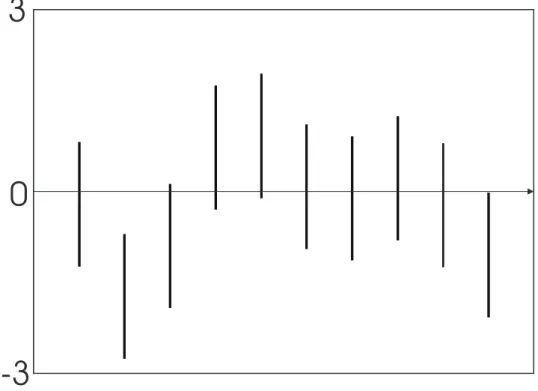
Ten simulated measurements were generated as follows. First ten noise-free measurements y were computed for k = 1; 2; : : : ; 10, at a “true” value of the parameter vector p = (1; 2) . Of course, this true value is not communicated to the estimation procedure. Noisy data y were then obtained by adding to y realizations of a random noise uniformly distributed in [¡1; 1]. The resulting data are presented in Figure 3, where the vertical bars indicate all possible values of the noise-free data when the e ’s are taken equal to¡1 and the ¹e ’s to 1. The feasible parameter set S is thus the set of all p’s that satisfy

8 > > > > > < > > > > > : sin(p ¤ (1 + p_!)) 2 [y ¡ 1; y + 1]; sin(p ¤ (2 + p_!)) 2 [y_!¡ 1; y_!+ 1]; ... ... ... sin(p ¤ (10 + p_!)) 2 [y "¡ 1; y "+ 1]: (7)

Sivia _{was used to characterize the part of S located in three search domains [p"] of} increasing size, namely [0; 2] £ [¡¼; ¼]; [0; 4] £ [¡2¼; 2¼] and [0; 8] £ [¡4¼; 4¼]. In all cases, the accuracy parameter "_" was taken equal to 0:008. The results, obtained in less than 10 seconds on a Pentium 133 MHz computer, are summarized by Figure 4, where the sizes of the frames are those of the search domains.

4.2

Identi…ability analysis

As is readily apparent from Figure 4, S consists of many disconnected components. Part of this fact may be explained by an identi…ability analysis [Wal82]. Roughly speaking, a model is said to be uniquely (or globally) identi…able if there is a single value of the parameter vector associated to any given behavior of the model output. From the equation

of the model (6), it is clear that any two vectors p and q of R such that p_!(t + p ) = q!(t + q ) + 2`¼; ` 2 Z, will lead to exactly the same behavior for all t’s. Then any q such

that q! = p! and q = !"_! will lead to the same behavior as p. The model considered

is therefore not uniquely identi…able, and if p2 S, then all vectors q of the form

q(`) = (p<sub>!</sub>;p ¡ 2`¼

p_! ); ` 2 Z; (8)

are also in S. This is why all the components of S are piled up with a pseudo periodicity given by 2¼=p_!. Note that this identi…ability analysis was not required for the estimation of the parameters by the method described in this chapter. Moreover, this estimation method allow us to obtain all models with similarly acceptable behaviors, and not just those that have exactly the same behavior.

5

Conclusions

Bounded-error estimation is an attractive alternative to more conventional approaches to parameter estimation based on a probabilistic description of uncertainty. When bounds are available on the maximum acceptable error between the experimental data and the corresponding model output, it is possible to characterize the set of all acceptable pa-rameter vectors by bracketing it between inner and outer approximations. Most of the results available in the literature require the model output to be linear in the unknown parameters to be estimated and only compute an outer approximation. The method de-scribed in this chapter is one of the very few that can be used in the nonlinear case. It provides both inner and outer approximations, which is important because the distance between these approximations is a precious indication about the quality of the description that they provide. We hope to have shown that the resulting methodology falls naturally into the framework of granular computing. The quality of the approximation obtained depends of the level of granularity, and a compromise must of course be struck between accuracy of description and complexity of representation.

Many important points could not be covered in this introductory material and still form the subject of ongoing research. They include the extension of the methodology to the estimation of the state vector of a dynamical system (or to the tracking of time-varying pa-rameters) [KJW98], and the robusti…cation of the estimator against outliers, i.e., against

data points for which the error should be much larger than originally thought, because, e.g., of sensor failure [JWD96], [KJWM99].

References

[Han92] E. R. Hansen. Global Optimization using Interval Analysis. Marcel Dekker, New York, 1992.

[HDM97] P. Van Hentenryck, Y. Deville, and L. Michel. Numerica. A Modeling Lan-guage for Global Optimization. MIT Press, 1997.

[JW93a] L. Jaulin and E. Walter. Guaranteed nonlinear parameter estimation from bounded-error data via interval analysis. Math. and Comput. in Simulation, 35:1923–1937, 1993.

[JW93b] L. Jaulin and E. Walter. Guaranteed nonlinear parameter estimation via interval computations. Interval Computation, pages 61–75, 1993.

[JW93c] L. Jaulin and E. Walter. Set inversion via interval analysis for nonlinear bounded-error estimation. Automatica, 29(4):1053–1064, 1993.

[JWD96] L. Jaulin, E. Walter, and O. Didrit. Guaranteed robust nonlinear para-meter bounding. In Proc. CESA’96 IMACS Multiconference (Symposium on Modelling, Analysis and Simulation), pages 1156–1161, Lille, July 9-12, 1996.

[KJW98] M. Kie¤er, L. Jaulin, and E. Walter. Guaranteed recursive nonlinear state estimation using interval analysis. In Proc. 37th IEEE Conference on Deci-sion and Control, pages 3966–3971, Tampa, December 16-18, 1998.

[KJWM99] M. Kie¤er, L. Jaulin, E. Walter, and D. Meizel. Nonlinear identi…cation based on unreliable priors and data, with application to robot localization. In A. Garulli, A. Tesi, and A. Vicino, editors, Robustness in Identi…cation and Control, pages 190–203, LNCIS 245, London, 1999. Springer.

[MNPLW96] M. Milanese, J. Norton, H. Piet-Lahanier, and E. Walter (Eds). Bounding Approaches to System Identi…cation. Plenum Press, New York, 1996.

[Moo66] R. E. Moore. Interval Analysis. Prentice-Hall, Englewood Cli¤s, New Jersey, 1966.

[Moo79] R. E. Moore. Methods and Applications of Interval Analysis. SIAM Publ., Philadelphia, 1979.

[Nor94] J. P. Norton (Ed.). Special issue on bounded-error estimation: Issue 1. Int. J. of Adaptive Control and Signal Processing, 8(1):1–118, 1994.

[Nor95] J. P. Norton (Ed.). Special issue on bounded-error estimation: Issue 2. Int. J. of Adaptive Control and Signal Processing, 9(1):1–132, 1995.

[Wal82] E. Walter. Identi…ability of state space models. Springer-Verlag, Berlin, 1982.

[Wal90] E. Walter (Ed.). Special issue on parameter identi…cations with error bounds. Mathematics and Computers in Simulation, 32(5&6):447–607, 1990.

[WP97] E. Walter and L. Pronzato. Identi…cation of Parametric Models from Ex-perimental Data. Springer-Verlag, London, 1997.

[WPL89] E. Walter and H. Piet-Lahanier. Exact recursive polyhedral description of the feasible parameter set for bounded-error models. IEEE Transactions on Automatic Control, 34(8):911–915, 1989.

Figure 1: Sequence of layers generated by sivia in Example 4; the black granules are inside S, the grey granules are outside S,

-3

3

0

Figure 3: Data bars for the parameter estimation example;

Figure 4: Characterizations of the part of S in [p ] obtained by sivia for increasing sizes of [p ]; dotted lines in the bottom two sub…gures indicate the correspondence between the frames of the sub…gures