Forests of hierarchical latent models for association genetics

HAL Id: hal-00503013

https://hal.archives-ouvertes.fr/hal-00503013

Submitted on 25 Jul 2010

HAL is a multi-disciplinary open access

archive for the deposit and dissemination of

sci-entific research documents, whether they are

pub-lished or not. The documents may come from

teaching and research institutions in France or

abroad, or from public or private research centers.

L’archive ouverte pluridisciplinaire HAL, est

destinée au dépôt et à la diffusion de documents

scientifiques de niveau recherche, publiés ou non,

émanant des établissements d’enseignement et de

recherche français ou étrangers, des laboratoires

publics ou privés.

genetics

Raphaël Mourad, Christine Sinoquet, Philippe Leray

To cite this version:

Raphaël Mourad, Christine Sinoquet, Philippe Leray. Forests of hierarchical latent models for

associ-ation genetics. 2010. �hal-00503013�

L

’I

N

-A

— KnOwledge and Decision (KOD) —

R

ESEARCH

R

EPORT

No hal-00503013

July 2010

Forests of hierarchical latent models for association

genetics

Raphaël Mourad

†, Christine Sinoquet‡, Philippe Leray†

†LINA, UMR CNRS 6241, Ecole Polytechnique de l’Université de Nantes, rue Christian Pauc, BP 50609,

44306 Nantes Cedex 3, France,

‡LINA, UMR CNRS 6241, Université de Nantes, 2 rue de la Houssinière, BP 92208, 44322 Nantes

Cedex, France

LINA, Université de Nantes – 2, rue de la Houssinière – BP 92208 – 44322 NANTES CEDEX 3

Tél. : 02 51 12 58 00 – Fax. : 02 51 12 58 12 – http

:

//www.sciences.univ-nantes.fr/lina/

Forests of hierarchical latent models for association

genetics

24p.

Les rapports de recherche du Laboratoire d’Informatique de Nantes-Atlantique sont disponibles aux formats PostScript®_{et PDF}®_{à l’URL :}

http://www.sciences.univ-nantes.fr/lina/Vie/RR/rapports.html

Research reports from the Laboratoire d’Informatique de Nantes-Atlantique are available in PostScript®_{and PDF}®_{formats at the URL:}

http://www.sciences.univ-nantes.fr/lina/Vie/RR/rapports.html

© July 2010 by

Raphaël Mourad

†, Christine Sinoquet‡, Philippe

Forests of hierarchical latent models for

association genetics

Raphaël Mourad

†, Christine Sinoquet‡, Philippe Leray†

raphael.mourad,christine.sinoquet,philippe.leray@univ-nantes.fr

Abstract

Genome wide association studies address the localization and identification of causal mutations responsible for com-mon, complex human genetic diseases. Nevertheless, this task has been revealed to be a formidable challenge because of the huge amount and the complexity of the data to analyze. At the frontier between machine learning and statistics, probabilistic graphical models, such as hierarchical Bayesian networks, are potentially powerful tools to tackle this issue. In this research work, we evaluate a novel method based on forests of hierarchical latent class models. We show the relevance of using this class of models for the purpose of genetic association studies.

We correct for multiple testing and cope with cardinality heterogeneity amongst the model’s latent variables. For this purpose, we design a layer-wise permutation procedure. We empirically prove, using both simulated and real data, the ability of the model’s latent variables to capture indirect genetic associations with the disease. Strong associations are evidenced between the disease and the causal genetic marker’s ancestor nodes in the forest. At the opposite, very weak associations are obtained regarding the causal genetic marker’s non-ancestor nodes.

1

Introduction

Thanks to their ability to capture (conditional) independences and dependences between variables, prob-abilistic graphical models (PGMs) offer an adapted framework for a fine modelling of relationships be-tween variables in an uncertain data framework [7]. A PGM is a probabilistic model relying on a graph representing conditional dependences within a set of random variables. Basically, this model provides a compact and natural representation of the joint distribution of the set of variables. Several subclasses of PGMs exist such as Markov random fields (MRFs) and Bayesian networks (BNs).

Formally, BNs are defined by a DAG G(X, E) and a set of parameters θ [11]. The set of nodes X= {X1, ..., Xn} represents n random variables and the set of edges E captures the conditional

depen-dences between these variables (i.e. the structure). The set of parametersθ is composed of conditional

probability distributionsθi = [P(Xi/P aXi)] where P aXidenotes nodei’s parents. Despite the fact that

the observed variables (OVs) are often sufficient to describe their joint distribution, sometimes, additional unobserved variables, also named latent variables (LVs), have a role to play. In this context, hierarchical Bayesian networks such as hierarchical latent class models (HLCMs) were proposed.

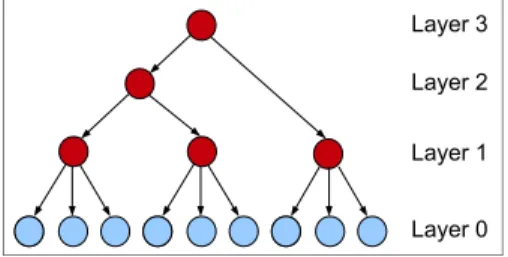
HLCMs are tree-shaped BNs where leaf nodes are observed while internal nodes are not. HLCMs were identified as a potentially useful class of BNs by Pearl [15] for various reasons. First, multiple LVs organized in a hierarchical structure allow high modelling flexibility (see Figure1) as well as struc-ture simplification to trees. Second, the attempt to learn these models can reveal latent causal strucstruc-tures. Third, HLCMs alleviate disadvantages of latent class models (LCMs), defined as containing a unique latent variable connected to each of the observed variables. In LCMs, observed variables are enforced to be independent, conditional on the latent variable [20]. In contrast, HLCMs relax the local independence (LI) assumption which is often violated by observed data. The applications of HLCMs are wide: clus-tering through the use of LVs, probabilistic inference in linear time or causal latent structure discovery. Few algorithms have been designed for learning such models [21,19] and fewer still for applications in association genetics [22].

Figure 1: Hierarchical latent class model. The light shade indicates the observed variables whereas the dark shade points out the latent variables.

Genetic markers such as SNPs are the key to dissecting the genetic susceptibility of complex diseases, such as asthma, diabetes, atherosclerosis and some cancers [9]. Indeed, they are used for the purpose of identifying combinations of genetic determinants which should accumulate among affected subjects. Generally, in such combinations, each genetic variant only exerts a modest impact on the observed phe-notype, the interaction between genetic variants and possibly environmental factors being determining in contrast. Decreasing genotyping costs now enable the generation of hundreds of thousands of genetic variants, or SNPs, spanning whole Human genome, accross cohorts of cases and controls. This scaling up to genome-wide association studies (GWAS) makes the analysis of high-dimensional data a hot topic.

Yet, the search for associations between single SNPs and the variable describing case/control status re-quires carrying out a large number of statistical tests. Since SNP patterns, rather than single SNPs, are likely to be determining for complex diseases, a high rate of false positives as well as a perceptible sta-tistical power decrease, not to speak of intractability, are severe issues to be overcome. As a possible solution, we propose to test associations using FHLCM’s LVs instead of SNPs.

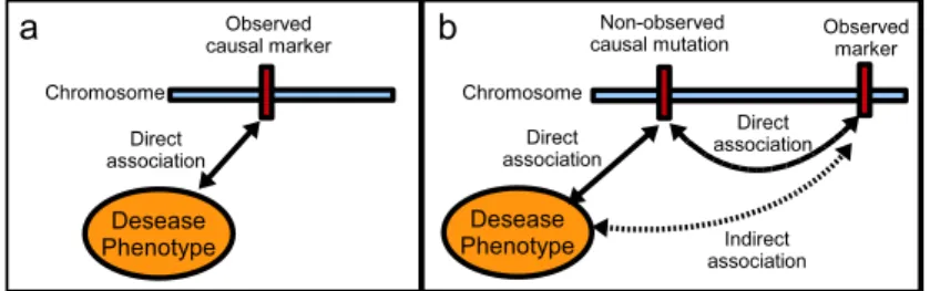
Exploiting the existence of statistical dependences between SNPs, also called linkage disequilibrium (LD), is the key to association study achievement [1]. Indeed, a causal variant may not be a SNP. For instance, insertions, deletions, inversions and copy-number polymorphisms may be causative of disease susceptibility. Nevertheless, a well-designed study will have a good chance of including one or more SNPs that are in strong LD with a common causal variant. In the latter case, indirect association with the phenotype, say affected/unaffected status, will be revealed (see Figure2).

Figure 2: a) Direct association between a genetic marker and the phenotype. b) Indirect association between a genetic marker and the phenotype.

Interestingly, LD appears crucial to reduce data dimensionality in GWASs. In eukaryotic genomes, LD is highly structured into the so-called "haplotype block structure" [13]: regions where correlation between markers is high alternate with shorter regions characterized by low correlation (see Figure3). Relying on this feature, various approaches were proposed to achieve data dimensionality reduction: testing association with haplotypes (i.e. inferred data underlying genotypic data) [16], partitioning the genome according to spatial correlation [14], selecting SNPs informative about their context, or SNP tags [4] (for other references, see [8] for example). Unfortunately, these methods do not take into account all existing dependences since they miss higher-order dependences.

Probabilistic graphical models offer an adapted framework for a fine modelling of dependences be-tween SNPs. Various models have been used for this peculiar purpose, mainly Markov fields [18] and Bayesian networks (BNs), with the use of hierarchical latent BNs (embedded BNs [12]); two-layer BNs with multiple latent (hidden) variables [22]. Although modelling SNP dependences through hierarchical BNs is undoubtedly an attractive lead, there is still room for improvement. Notably, scalability remains a crucial issue.

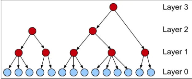
In a previous article [10], we designed an original framework dedicated to genetic data analysis, rely-ing on forests of HLCMs, namely FHLCMs (see Figure4). Considering genetic markers which describe DNA variability among individuals, our final aim is dissecting the genetic susceptibility of complex dis-eases. FHLCMs allow to model a larger set of configurations than HLCMs do. Typically, an HLCM is limited to represent clusters of close dependent variables. Actually, in this model, variables are con-strained to be dependent upon one another, either directly or indirectly. But realistic modelling requires a more flexible framework. Indeed, the vast majority of statistical dependences, also called linkage disequi-librium (LD), is observed between SNPs (Single Nucleotide Polymorphisms), or genetic markers, which

7

Figure 3: LD plot (matrix of pairwise dependences between genetic markers or linkage disequilibrium). Human genome, chromosome2, region [234 357kb - 234 457kb]. For a pair of SNPs, the colour shade is

all the darker as the correlation between the two SNPs is high.

are close to one another, on the chromosome. LD is rarely observed for SNPs distant by more than500 kb [6]. We argued that the FHLCMs can offer several advantages for genetic data analysis, in particular for genome-wide association studies (GWASs). For instance, FHLCMs’ hierarchical structure supported by LVs allows flexible information synthesis, thus efficiently reducing the data dimensionality. Indeed, in an FHLCM, the different layers provide several degrees of reduction, which allow zooming in through narrower and narrower regions in search for stronger associations with the disease. Another promising property of the FHLCMs relies on their ability to allow a simple test of direct dependence beween an observed variable and a target variable such as the phenotype, conditional on the latent variable, parent of the observed variable. Note that the phenotype variable is not included in the FHLCM. In the context of GWASs, this test helps finding the markers which are directly associated with the phenotype, i.e. causal markers, should there be any.

Figure 4: Forest of hierarchical latent class models. See Figure1for node nomenclature.

In the present work, we apply our new genetic association method based on FHLCMs, to empirically show that the FHLCMs are relevant to detect indirect genetic associations with the disease. From now on, we name indirect genetic association any dependence between a causal SNP’s ancestor node (abbreviated as CA) of the FHLCM and the disease. Such an indirect association is due to the fact that a CA is likely to capture the information of a causal SNP. The capture of indirect genetic association is at the basis of our original genetic association approach: the identification of CA nodes helps to point out the causal marker, since the latter is one of the leaves (observed variables) of a tree rooted in a CA node. For our purpose, the performence of the FHLCM-based method is evaluated using both simulated and real genotypic data. Simulations are generated under different scenarii varying in minor allele frequencies (MAFs), geno-type relative risks (GRRs) and disease models. The real data analysis considers the well-studied region

flanking the CYP2D6 human gene [5]. In order to assess the significance of the associations, we also adapted a permutation procedure dedicated to the computation of p-value thresholds, each one specific to a FHLCM’s layer.

This paper is organized as follows: in the second Section, we provide a quick insight of the CFHLC algorithm dedicated to FHLCM learning; the third Section describes the evaluation protocol implemented to assess the relevance of our approach when applied for association studies; the fourth Section details our results and discusses them. Finally, the last Section highlights the contribution of our work and gives directions for future works.

2

A short tour of CFHLC algorithm

In a previous paper [10], we described a scalable algorithm, named CFHLC, conceived for learning both structure and parameters of FHLCMs dedicated to genome-wide data analysis. The learning is performed through an adapted agglomerative hierarchical clustering (AHC) procedure: (i) at each agglomerative step, a clique partitioning method is used to identify cliques of variables (i.e. statistically dependent vari-ables); (ii) each such clique, if relevant, is intended to be subsumed into an LV, through an LCM. For each LCM, parameter learning using expectation-maximization (EM) algorithm and missing data imputation through probabilistic inference (for the latent variable) are performed. Iterating these two steps yields a hierarchical structure.

In other words, latent variables capture the information born by underlying observed variables (e.g. genetic markers). To their turn, latent variables can be synthetized through additional latent variables, and so on. During the agglomerative construction, the number of layers is determined thanks to a decay information criterion: each LCM corresponding to a clique is checked for carrying sufficient information about the subsumed variables.

The reader interested in the detailed algorithm is referred to the aforementioned paper [10]. In par-ticular, three ingredients of algorithm CFHLC - node partitioning, imputation of LV values and control of information decay - are described therein. It has to be emphasized that the theoretical framework proposed is generic and that, regarding implementation, any strategy implementing one of the previous ingredients may be plugged into the generic scheme. For a quick insight, the sketch of the algorithm is presented in Figure5. Stage1 implements genome scanning through contiguous windows encompassing

up to some hundreds of SNPs. Stage2 identifies cliques of pairwise-dependent variables, the dependence

being controlled by a given threshold. The next phase (3) builds as many LCM models (i.e. as many LVs)

as there are such previous cliques identified. The LCM parameters are learnt through phase4, which

subsequently allows the imputation of the values of each LV for all individuals considered in the study. A validation stage (5) controls that the unescapable information decay accompanying the subsuming

pro-cess is not too drastic. Now, such LVs satisfying the validation procedure are considered as observed variables for the next step of the AHC procedure (stages2 through 5). The AHC process stops when

no more clique or relevant LCM is identified. Then, the FHLCM corresponding to the current window is constructed through a procedure growing trees from leaves to root, starting from the nodes in initial

0 layers (i.e. layers only including initial OVs) (phase 6). Finally, the FHLCM modelling the studied

9

P1

2: Clique partitioning of variables Ci

3: Construction of an LCM (DAG) for each clique of

size ≥ 2

4: Learning of parameters and imputation of values

for each parent Pj 5: Validation of LCMs

based on information criterion C and update of the matrix of observations

1: Split the sequence into windows Window SNP sequence 6: Construction of the FHLCM from the LCMs C3 C1 C2 C5 C4 C7 C6 P2 C2 C3 C1 P1 C6 C7 C4 C5 P2

7: Union of the different FHLCMs built for each window

C6 C7

Figure 5: Scheme of algorithm CFHLC. The light shade indicates the observed variables whereas the dark shade points out the latent variables.

3

Evaluation of the CFHLC approach

3.1

Protocol description

Relying on data for which the causal SNP is known, the guide line of our evaluation protocol consists of the following steps: (i) build the FHLCM corresponding to the genome or genomic region under study, (ii) carry on an association test between the phenotype variableY and each node of the FHLCM, (iii)

compare the p-values obtained for three node sets: a set reduced to the causal SNP (i.e. a leaf of the FHLCM); CAs, the set of causal SNP’s ancestor nodes and CNAs, the set of causal SNP’s non-ancestor nodes.

Illustrating the trends for all three node sets has first been achieved through graphical visualization: we have plotted the mean p-values obtained for the causal SNP, the CAs of a given layer and the CNAs belonging to the same layer in the FHLCM. Furthermore, two tests have been performed to confirm or invalidate the dissimilarity of the p-value distributions relative to both CA and CNAs sets. We first used a non-parametric standard test, the Wilcoxon rank-sum test.

Recently, a method, called local FDR (false discovery rate), has been proposed to estimate the specific probability, given the p-value, for being under the null hypothesis [3]. The method relies on a mixture

distribution of p-values depending on the unobserved status of the null hypothesis (true or false). In the present work, the local FDR method has proven useful to finely compare the proportion of CAs and CNAs under the alternative hypothesis.

3.2

Assessment of genetic associations adapted to the FHLCM framework

To measure the association strength between a variableX of the FHLCM (OV or LV) and the phenotype Y , we used standard tests for independence. We applied the G2 _{test instead of the well-knownChi}2

test. Indeed, the former corresponds to the likelihood ratio test (LRT) whereas the latter is just an ap-proximation of the LRT. For samples of reasonable sizes, theG2test and theChi2 test will lead to the same conclusions. But for relatively small sample sizes (below300 individuals) as is the case for the real

dataset analyzed, large divergences between results are expected. For theG2test, the degree of freedom is(n − 1) × (m − 1), in our case (n − 1), where n is the cardinality of X and m is the cardinality of Y

(here, constant and equal to2).

Due to information decay through bottom to top, in an FHLCM, it would be nonsense to apply the same threshold to assess significance for two variables belonging to different layers. Therefore, to assess the significance of associations, we had to implement a specific permutation procedure dedicated to the computation of the per-test type I error rateα′_{, in order to control the family-wise type I error rateα .}

α controls the probability to make one or more false discoveries among all hypotheses when performing

multiple association tests. For a givenα value, the larger the number of variables to be tested, the lower α′ must be. An advantage of our FHLCM strategy relies on the fact that there are less variables in the higher layers than in the lower ones. Thus, an increase ofα′is expected as the layer level increases.

In the standard permutation procedure dedicated to this control purpose [2], the labels of the target variableY (in genetic association studies, the phenotype) are permuted a given number of times, amongst

individuals, which provides a set of permutationsP. For each permutation, a test between Y and each

variable tested for association is run, e.g. a Chi2 _{test, and the maximum statisticmax(T ) obtained}

over all tests is saved. When the number of permutations is sufficiently large, themax(T ) distribution

represents a good empirical approximation of the null hypothesis distribution, that is the no dependence hypothesis. In our model, LVs may present various cardinalities, thus requiring association tests involv-ing different degrees of freedom. Therefore, we can not compare themax(T ) statistics with one another.

That is the reason why we had to adapt the standard permutation method to this characteristic. The adap-tation is straightforward: instead of relying on the maximum statistic distribution, we use the distribution of minimum p-values. Indeed, p-values are comparable, since the degree of freedom is taken into account in a p-value and the minimum p-value can replace the maximum statistic max(T ) in the distribution

construction.

The adapted permutation procedure is described in Algorithm1. The procedure performsnp

permu-tations. For each permutation, and each FHLCM’s layer, independence tests are run for any variableXv

belonging to FHLCM’s layerℓ and the target variable Y . For each permutation, the minimum of the

p-values over all variables belonging to FHLCM’s layerℓ is identified, which will constitute the distribution

of minimal p-values for this layer. Given a specified family-wise error rateα, this distribution then allows

to extract the correspondingα′_{threshold. Thisα}′_{value, specific to each layer, is to be compared with the}

p-value resulting from the association test between variableXv(belonging to layerl) and Y . Thus can

be assessed association significance, corrected for family-wise type I error, or should one write instead, controlled for layer-wise type I error.

11

Algorithm 1 PermutationProcedure(X, DX, Y, DY, np, α)

INPUT:

X, DX: a set ofnvcandidate variables (observed or latent)X= X1, ..., Xnvand the corresponding data observed or imputed forn individuals,

Y, DY: a target variableYand the corresponding data observed fornindividuals,

np: the number of permutations,

α: the family-wise error rate.

OUTPUT:

{α′_{(1), ..., α}′_(n

ℓ)}: the set of per-test error rates respectively computed for layersltonℓ. 1: forℓ= 1tonℓ

2: distribminP V alues(ℓ)← ∅ 3: end for

4: forp= 1tonp

5: D_Yp← permuteLabels(DY) 6: forℓ= 1tonl

7: pV alues(p, ℓ)← ∅

8: for each variableXvin layerℓ

9: pV aluep, ℓ, v← runAssociationT est(Xv, DYp) 10: pV alues(p, ℓ)← pV alues(p, ℓ) ∪ pV aluep, ℓ, v 11: end for

12: distribminP V alues(ℓ)← distribminP V alues(ℓ)∪ minXv(pV alues(p, ℓ)) 13: end for 14: end for 15: forℓ= 1tonl 16: α′_{(ℓ)← quantile(distrib} minP V alues(ℓ), α) 17: end for

4

Results and discussion

Algorithm CFHLC has been implemented in C++, relying on the ProBT library dedicated to BNs (http:// bayesian-programming.org). CFHLC was run on a standard personal computer (3 GHz, 2 GB RAM).

We have performed intensive testing to evaluate the relevance of using FHLCMs for genetic associa-tion purpose. Tests have been performed both on simulated and real biological data. To implement

layer-wise type I error correction,α threshold has been set to 0.05, with a number of permutations

equal to1000, quite standard values for this aim. The local FDR-based method has been run through

Kerfdr, an R package implementing a semi-parametric approach based on kernel estimators (http://cran.r-project.org/web/packages/kerfdr/).

We will display the−log10(p-value) values instead of the p-values themselves. The−log10(p-value)

values near0 point out independence and the previous indicator increases with the strength of the

depen-dence.

4.1

Simulations

4.1.1 Generation of realistic genetic data

To assess the ability of FHLCM’s LVs to capture indirect genetic associations, we have simulated geno-typic and phenogeno-typic data under various scenarii. In particular, we have considered different scenarii combining various minor allele frequencies, genotype relative risks and disease models. We have repli-cated each scenario100 times. SNP data without missing values have been generated using software

of the HapMap phase II coming from U.S. residents of northern and western European ancestry (CEU) (http://hapmap.ncbi.nlm.nih.gov/). The simulated data has been generated for1000 controls and 1000

cases (unrelated individuals) and consists of unphased genotypic data relative to a1.5 M b region

con-taining around100 SNPs. Among the simulated SNPs, HAPGEN selects one SNP to be the causal marker

associated with the simulated phenotype (affected/unaffected). The MAF (minor allele frequency) at the causal SNP is specified to belong to interval [0.1-0.2], [0.2-0.3] or [0.3-0.4]. Different heterozygous genotype relative risks are considered: 1.4, 1.6 or 1.8. The disease model is specified among additive,

dominant, multiplicative or recessive. Combining all previous conditions led to testing3 × 3 × 4 scenarii.

Quality control of genotypic data has been carried out: SNPs with MAF less than0.05 and SNPs deviant

from the Hardy-Weinberg Equilibrium (HWE) with a p-value below0.001 have been removed.

4.1.2 Comparing CA nodes to CNA nodes

In the following, the data analysis may entail the generation of up to7 layers in the FHLCM. We will not

report results obtained for layers with numbers above3: indeed, such layers do not provide sufficient data

to compute representative medians or draw informative boxplots. On average, over all3600 FHLCMs (36

scenarii× 100 replicates), the percentages of nodes are distributed as follows: 89.1% in layer 0, 9.5% in

layer1, 1.2% in layer 2 and 0.2% in layer 3.

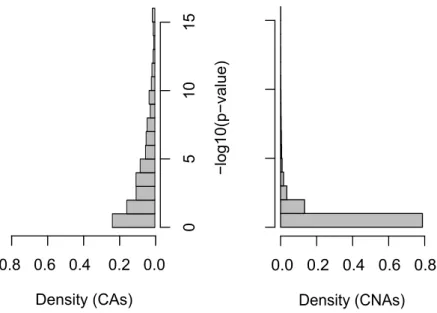
Figure6 compares the histograms of−log10(p-value) values resulting from association tests ofY

with the CAs and with the CNAs, respectively. The comparison of these two histograms reveals a large dissimilarity between the two distributions. The majority (70%) of −log10(p-value) values relative to

CAs is greater than 1, whereas it is the case for only 19% for CNAs. Indeed, we observe that large −log10(p-value) values (e.g., greater than5) are common for the former and are very rare for the latter.

The Wilcoxon rank-sum test shows a p-value less than10−16, which confirms that CA and CNA p-values follow two different distributions.

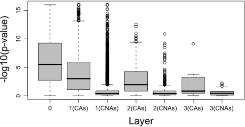
Now distinguishing between layers, Figure7more thoroughly describes the−log10(p-value) values

observed for the tests relative to CAs and CNAs. Layer0 represents the association test between the

phe-notype and the causal SNP and serves as the reference value. We remind the reader that there are as many association tests between causal marker and phenotype as there are different scenarios (36) in our

evalu-ation protocol. In Figure7, we observe that the association strength with CAs slowly decreases when the layer number increases, whereas the association strength with CNAs dramatically falls to−log10(p-value)

values below0.4, corresponding to p-values greater than 0.4. Although CNAs reveal false positive

asso-ciations (less than10% have a p-value below 0.01), these results clearly highlight a general trend: indirect

associations are captured by the CAs while it is not the case for a large majority of CNAs.

4.1.3 CA versus CNA node comparison including significance assessment

Figure9emphasizes the general trend of−log10(p-value) values on CAs and CNAs, and compares the

median −log10(p-value) value obtained for each layer to the corresponding value associated with the

significance thresholdα′_{specific to this layer (see Subsection3.2). Figure9reveals that up to the second}

layer, significant associations are identified for CAs. In contrast, regarding CNAs, in all layers, median

−log10(p-value) values are smaller than the corresponding−log10(α′) values. Focusing on the CNA

distribution, the rate of p-values lower thanα′_{value (false positives) is4.7%.}

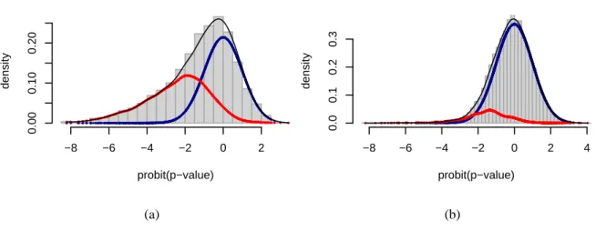
Relying on the local FDR method, Figure8displays the trend for CA and CNA nodes and confirms the aforedescribed contrast between both node sets. Regarding CA nodes, known to be associated with

13 Density (CNAs) 0.0 0.2 0.4 0.6 0.8

Figure 6: Histograms of−log10(p-value) values resulting from association tests between the phenotype

and the causal SNP’s ancestor nodes or between the phenotype and the causal SNP’s non-ancestor nodes. These histograms compile all studied scenarii: MAF ([0.1-0.2], [0.2-0.3] and [0.3-0.4]), GRR (1.4, 1.6

and1.8) and disease model (additive, dominant, multiplicative and recessive). The X-axis indicates the

proportion of nodes showing a−log10(p-value) value in the corresponding interval indicated by the

Y-axis.

the disease, the probability that the association test be observed under the alternative hypothesis is pre-vailing, as expected: mixture and alternative hypothesis densities are close to one another. In the right section of Figure8(a), the presence of the small peak related to the (true) null hypothesis calls for the following comment: for the p-values corresponding to the concerned probit range ([−2, 2]), the

proba-bility that this p-value be observed under the true null hypothesis is not close to0 as it is elsewhere in

the figure; indeed, this probability is greater than the probability of the alternative hypothesis for p-value probit interval[0, 2]. The pointed area designates false negatives. In contrast, in Figure8(b) showing the trend for CNAs, as expected, the curves relative to mixture and true null hypothesis are superimposed. Knowing that CNAs are not associated with the disease, the curve related to false null hypothesis points out false positives.

The existence of false positives (FPs) can partly be explained by the presence of indirect dependences between the causal SNP and the CNAs of the causal tree (the tree containing the causal SNP), nodes abbreviated as CT-CNAs. At the opposite, no FPs are expected for CNAs present in the non-causal trees (NCT-CNAs). Actually, more than73% of FPs are CT-CNAs, which represents only 21% of CNAs. The

rate of FPs in CT-CNAs is16.07% whereas it is 10 times less in NCT-CNAs.

When applying the local FDR method to CT-CNA and NCT-CNA p-values, we confirm that the mixture distributions of both hypotheses greatly differ: a major part of CT-CNA p-values follows the alternative hypothesis (see Figure10(a)), while it is the case for only a very small part of NCT-CNA

0 1(CAs) 1(CNAs) 2(CAs) 2(CNAs) 3(CAs) 3(CNAs) 0 5 10 15

Layer

-lo

g1

0(

p

-val

ue

)

Figure 7: Boxplot of−log10(p-value) values for the different layers of the FHLCM, resulting from

as-sociation tests between the phenotype and the causal SNP’s ancestor nodes or between the phenotype and the causal SNP’s non-ancestor nodes. Layer0 indicates the result of the association test between the

phenotype and the causal SNP (mean over all scenarii). See Figure6for details about the scenarii.

probit(p−value) density −8 −6 −4 −2 0 2 0.00 0.05 0.10 0.15 probit(p−value) density −8 −6 −4 −2 0 2 4 0.00 0.15 0.30 (a) (b)

Figure 8: Mixture distributions ofprobit(p-values) depending on the unobserved status of the null

hy-pothesis (true or false) - CA nodes versus CNA nodes, simulated data, all scenarii -. (a) Mixture distribu-tion learnt for CA p-values. (b) Mixture distribudistribu-tion learnt for CNA p-values. See Figure6for definitions of CA and CNA nodes and details about the scenarii. The distribution under the true null hypothesis corresponds to the thick (blue) line, whereas the distribution relative to the false null hypothesis is dis-played through a thin (red) line. The third line corresponds to the mixture. Theprobit tranformation is

the inverse cumulative distribution function associated with the standard normal distribution.

p-values (see Figure10(b)). Thus, we conclude that a prominent part of false positive associations are due to indirect dependences between CT-CNAs and the phenotype.

15 0 1 2 3 1 2 3 4 5 Layer −log1 0(p−value ) C ausal SN P C As C C N As

av

Per-test error rate: -log10(α')

Median -log10(p-value)

Figure 9: Median−log10(p-value) values for the different layers of the FHLCM, resulting from tests of

association with the phenotype (for the definition of error rateα′, see last paragraph of3.2). CAs: causal SNP’s ancestor nodes; CNAs: causal SNP’s non-ancestor nodes. See Figure6 for more details about layer0. probit(p−value) density −8 −6 −4 −2 0 2 0.00 0.10 0.20 probit(p−value) density −8 −6 −4 −2 0 2 4 0.0 0.1 0.2 0.3 (a) (b)

Figure 10: Mixture distributions ofprobit(p-values) depending on the unobserved status of the null

hy-pothesis (true or false) - CT-CNA nodes versus NCT-CNA nodes, simulated data, all scenarii -. (a) Mix-ture distribution learnt for CT-CNA p-values. (b) MixMix-ture distribution learnt for NCT-CNA p-values.See Figure6for definitions of CT-CNA and NCT-CNA nodes and details about the scenarii. The distribution under the true null hypothesis corresponds to the thick (blue) line, whereas the distribution relative to the false null hypothesis is displayed through a thin (red) line. The third line corresponds to the mixture. The

probit tranformation is the inverse cumulative distribution function associated with the standard normal

distribution.

4.1.4 Comparison between various genetic scenarii

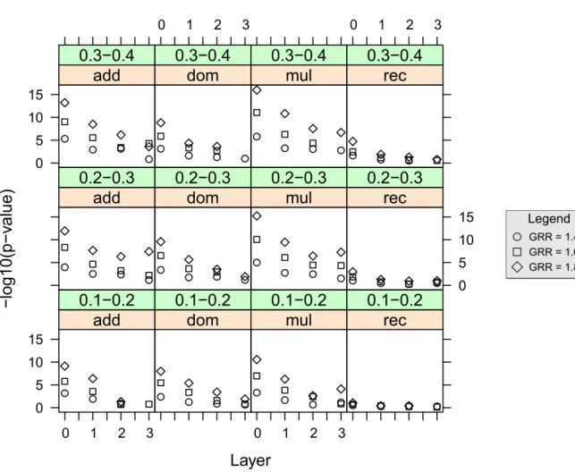
We recall the reader that we have evaluated the behaviour of FHLCM’s LVs under several genetic config-urations: minor allele frequency (MAF) range at the causal SNP between [0.1-0.2], [0.2-0.3] or [0.3-0.4]; heterozygous genotype relative risk of1.4, 1.6 or 1.8; additive, dominant, multiplicative or recessive

causal SNP, CAs and CNAs, now distinguishing between all36 scenarii. Figures11and12respectively focus on CAs and causal SNPs, and CNAs and causal SNPs. On average, similar tendencies are observed over all scenarii: the association strength continuously drops from bottom to fourth layer; in the case of CNAs, an overwhelming majority of results point out absence of association, whichever the FHLCM’s layer concerned.

Layer

−log1

0(p−v

alue

)

add

0.1−0.2

dom

0.1−0.2

mul

0.1−0.2

rec

0.1−0.2

add

0.2−0.3

dom

0.2−0.3

mul

0.2−0.3

rec

0.2−0.3

add

0.3−0.4

dom

0.3−0.4

mul

0.3−0.4

rec

0.3−0.4

Figure 11:−log10(p-value) median values for the different layers of the FHLCM, resulting from

associ-ation tests between the phenotype and the causal SNP’s ancestor nodes. The different windows represent possible genetic scenarii. At the top of each window, the range of the simulated causal SNP’s minor allele frequency and the disease model assumption are indicated (additive, dominant, multiplicative or recessive). The three different symbols used refer to as many genotype relative risks considered for the simulated causal SNP (see Legend). The result for layer0 corresponds to tests of association between the

17

Layer

−log1

0(p−v

alue

)

add

0.1−0.2

dom

0.1−0.2

mul

0.1−0.2

rec

0.1−0.2

add

0.2−0.3

dom

0.2−0.3

mul

0.2−0.3

rec

0.2−0.3

add

0.3−0.4

dom

0.3−0.4

mul

0.3−0.4

rec

0.3−0.4

Figure 12: Median of−log10(p-value) values for the different layers of the FHLCM, resulting from

tests of association between the phenotype and the causal SNP’s non-ancestor nodes. See Figure11for parameter description and more details about layer0.

When considering the easiest case (MAF range= 0.3-0.4, GRR = 1.8 and multiplicative model),

over all layers, the CAs present strong associations (−log10(p-value) > 7). Regarding a less ideal

but more plausible configuration (MAF range= 0.2-0.3, GRR = 1.6 and additive model), the median −log10(p-value) value computed for CAs decreases from8.3 at layer 0, to reach 4.6, 3.2 and 2.2 at layers

1, 2 and 3, respectively. On the contrary, when the model is recessive, the association with the causal SNP

is low and the CAs can not capture anything (similar results are obtained with most of the methods ded-icated to association studies). As regards the causal SNP’s non-ancestors, null associations are reported in all configurations.

0 1(CAs) 1(CNAs) 2(CAs) 2(CNAs) 3(CAs) 0 2 4 6 8 1 0 12 1 4

Layer

-lo

g1

0(

p

-val

ue

)

Figure 13: Boxplot of −log10(p-value) values for the different layers of the FHLCM, resulting from

tests of association of the phenotype with the causal SNP’s ancestor nodes or with the causal SNP’s non-ancestor nodes. Layer0 represents the tests of association between the phenotype and the causal SNP

(marker19). In layer 3, no CNAs are observed in the FHLCMs.

4.2

Application to real data

We have evaluated our hierarchical Bayesian network approach on a real genotypic dataset from a890 kb region flanking the CYP2D6 gene on human chromosome 22q13. This gene has been shown to play

a confirmed role in drug metabolism [5]. The studied genomic region consists of32 SNP markers

geno-typed for268 individuals and has been downloaded from the R package graphminer developed by Verzilli

and collaborators [18]. This genomic region has been used in several studies, to test proposed LD-based methods dedicated to fine mapping. Strong evidence has been brought that the SNP19 at position 550 kb

is the marker most significantly associated with CYP2D6 gene (whose "location" is referred to as525.3 kb position) [17]. For this reason, we considered the SNP19 as the causal marker in our experiment.

To take into account the stochastic nature of our algorithm (random initialization of parameters dur-ing the EM algorithm), we present the results of1000 runs (5.4 s per run on average, on a standard PC

computer (3 GHz, 2 Go RAM)).

On average, over all1000 FHLCMs (1000 replicates), the percentages of nodes are distributed as

follows:82.62% in layer 0, 16.89% in layer 1, 0.39% in layer 2 and 0.10% in layer 3. Figure13shows the−log10(p-value) values of association tests relative to CAs and CNAs. As expected in view of

exper-iments led on simulated data, the CAs succeed in capturing indirect association, in particular in layer1,

with a median value of5.5, corresponding to p-values lower than 5.10−6_{. In the other layers, the strength}

of associations is lower but remains relatively high as in layer2 showing a median value of 4, equivalent

to a p-value of10−4. As previously seen, when we focus on CNAs, we observe very few strong associa-tions. The majority of p-values (over80%) are greater than 0.01.

Finally, in addition to intensive evaluation performed on simulated benchmarks, similar tests con-ducted on real data confirm that the FHLCM-based method is relevant to detect causal regions.

19

5

Conclusion

Using both intensive testing on simulated and real genetic data, the research work reported here demon-strates the ability of FHLCM’s latent variables to guarantee data dimension reduction while allowing efficient identification of genetic associations. In our hierarchical Bayesian network proposal, the two keys to efficient association capture are the following ones: (i) the causal SNP’s ancestor nodes suc-ceed in capturing indirect associations with the phenotype; (ii) in contrast, the causal SNP’s non-ancestor nodes globally show very weak associations. These two characteristics allow to distinguish between true and false indirect genetic associations. We have addressed the efficiency question, performing associa-tion studies simulated under four realistic disease models, three disease severities and three ranges for causal marker’s minor allele frequency. We have adapted correction for multiple hypothesis testing to a multi-layered framework. We have also started investigations connected to power analysis, relying on the local FDR approach.

Complementary points will be addressed in future works. First, we will investigate whether bene-fitting from the ability of FHLCMs to encode conditional independences between variables could help reinforcing the dismissing of false indirect associations: we will evaluate an association analysis proce-dure implementing, for instance, tests for conditional independence.

Second, we will adapt our Bayesian network-based method to tackle genome-wide association stud-ies. A protocol involving far more intensive tests as in the present preliminary work is planned, relying on both genome-scale simulated and real data. In addition, we will go deeper into the study of our method’s power to identify robust associations between a causal SNP and a binary quantitative trait.

Finally, the ability of FHLCMs to implement relevant modelling for biological data will be further investigated to cope with more complex association analyses. Indeed, in the present work, we made the assumption that the causal genetic factor restrains to a unique marker. But reality is more complex. The causal genetic factor might be the share haplotype, carrying the mutation which appeared in the past, for an ancestor individual. In this case, the latent variables in our hierarchical model could also be able to represent this type of causal genetic factor. Thus, beside their subsumption role, latent variables might play a role in interpreting association studies.

References

1. David J. Balding. A tutorial on statistical methods for population association studies. Nature

Genetics, 7:781–790, 2006.

2. Phillip I. Good. Permutation, parametric, and bootstrap tests of hypotheses. Springer, 3rd edition, December 2004.

3. Mickael Guedj, Stephane Robin, Alain Celisse, and Gregory Nuel. Kerfdr: a semi-parametric kernel-based approach to local false discovery rate estimation. BMC bioinformatics, 10:84+, March 2009.

4. Han, B., Kang, H. M., Seo, M. S., Zaitlen, N., Eskin, and E.. Efficient association study design via power-optimized tag snp selection. Annals of Human Genetics, 72(6):834–847, November 2008.

5. L. K. Hosking, P. R. Boyd, C. F. Xu, M. Nissum, K. Cantone, I. J. Purvis, R. Khakhar, M. R. Barnes, U. Liberwirth, K. Hagen-Mann, M. G. Ehm, and J. H. Riley. Linkage disequilibrium mapping identifies a 390 kb region associated with cyp2d6 poor drug metabolising activity. The

Pharmacogenomics Journal, 2(3):165–175, 2002.

6. International HapMap Consortium. The international hapmap project. Nature, 426(6968):789– 796, December 2003.

7. Daphne Koller and Nir Friedman. Probabilistic Graphical Models: Principles and Techniques

(Adaptive Computation and Machine Learning). The MIT Press, August 2009.

8. Y. Liang and A. Kelemen. Statistical advances and challenges for analyzing correlated high di-mensional snp data in genomic study for complex diseases. Statistics Surveys, 2:43–60, 2008. 9. A. P. Morris and L. R. Cardon. Handbook of statistical genetics, volume 2, chapterWhole genome

association, pages 1238–1263. Wiley Interscience, 3rd edition, 2007.

10. Raphael Mourad, Christine Sinoquet, and Philippe Leray. Learning hierarchical bayesian net-works for genome-wide association studies. In 19th International Conference on Computational

Statistics (COMPSTAT), pages 549–556, 2010.

11. Patrick Naïm, Pierre-Henri Wuillemin, Philippe Leray, Olivier Pourret, and Anna Becker. Réseaux

bayésiens. 3 edition, 2007.

12. Ara V. Nefian. Learning snp dependencies using embedded bayesian networks. In IEEE

Compu-tational Systems, Bioinformatics Conference, 2006.

13. N. Patil, A. J. Berno, D. A. Hinds, W. A. Barrett, J. M. Doshi, C. R. Hacker, C. R. Kautzer, D. H. Lee, C. Marjoribanks, D. P. McDonough, B. T. Nguyen, M. C. Norris, J. B. Sheehan, N. Shen, D. Stern, R. P. Stokowski, D. J. Thomas, M. O. Trulson, K. R. Vyas, K. A. Frazer, S. P. Fodor, and D. R. Cox. Blocks of limited haplotype diversity revealed by high-resolution scanning of human chromosome 21. Science (New York, N.Y.), 294(5547):1719–1723, November 2001.

14. Cristian Pattaro, Ingo Ruczinski, Daniele M. Fallin, and Giovanni Parmigiani. Haplotype block partitioning as a tool for dimensionality reduction in snp association studies. BMC Genomics, 9:405, August 2008.

15. Judea Pearl. Probabilistic reasoning in intelligent systems : networks of plausible inference. Mor-gan Kaufmann, Santa Mateo, CA, USA, September 1988.

16. D. J. Schaid. Evaluating association of haplotypes with traits. Genetic Epidemiology, 27:348–364, 2004.

17. Ioanna Tachmazidou, Claudio J. Verzilli, and Maria D. Iorio. Genetic association mapping via evolution-based clustering of haplotypes. PLoS Genetics, 3(7):e111+, July 2007.

18. Claudio J. Verzilli, Nigel Stallard, and John C. Whittaker. Bayesian graphical models for genome-wide association studies. The American Journal of Human Genetics, 79:100–112, 2006.

19. Yi Wang, Nevin Lianwen Zhang, and Tao Chen. Latent tree models and approximate inference in bayesian networks. Machine Learning, 32:879–900, 2006.

20. Nevin L. Zhang. Hierarchical latent class models for cluster analysis. The Journal of Machine

21

21. Nevin L. Zhang and Thomas Kocka. Efficient learning of hierarchical latent class models. In

Pro-ceedings of the 16th IEEE International Conference on Tools with Artificial Intelligence (ICTAI),

pages 585–593, 2004.

22. Y. Zhang and L. Ji. Clustering of snps by a structural em algorithm. In International Joint

Forests of hierarchical latent models for association

genetics

Raphaël Mourad

†, Christine Sinoquet‡, Philippe Leray†

Abstract

Genome wide association studies address the localization and identification of causal mutations responsible for com-mon, complex human genetic diseases. Nevertheless, this task has been revealed to be a formidable challenge because of the huge amount and the complexity of the data to analyze. At the frontier between machine learning and statistics, probabilistic graphical models, such as hierarchical Bayesian networks, are potentially powerful tools to tackle this issue. In this research work, we evaluate a novel method based on forests of hierarchical latent class models. We show the relevance of using this class of models for the purpose of genetic association studies.

We correct for multiple testing and cope with cardinality heterogeneity amongst the model’s latent variables. For this purpose, we design a layer-wise permutation procedure. We empirically prove, using both simulated and real data, the ability of the model’s latent variables to capture indirect genetic associations with the disease. Strong associations are evidenced between the disease and the causal genetic marker’s ancestor nodes in the forest. At the opposite, very weak associations are obtained regarding the causal genetic marker’s non-ancestor nodes.

LINA, Université de Nantes 2, rue de la Houssinière