HAL Id: hal-01326442
https://hal.archives-ouvertes.fr/hal-01326442
Submitted on 3 Jun 2016
HAL is a multi-disciplinary open access
archive for the deposit and dissemination of
sci-entific research documents, whether they are
pub-lished or not. The documents may come from
teaching and research institutions in France or
abroad, or from public or private research centers.
L’archive ouverte pluridisciplinaire HAL, est
destinée au dépôt et à la diffusion de documents
scientifiques de niveau recherche, publiés ou non,
émanant des établissements d’enseignement et de
recherche français ou étrangers, des laboratoires
publics ou privés.
Analytical model of two level scheduling algorithm for
WiMAX networks
Zeeshan Ahmed, Salima Hamma
To cite this version:
Zeeshan Ahmed, Salima Hamma. Analytical model of two level scheduling algorithm for WiMAX
networks. International conference on Wireless Networks and Mobile Communications (WINCOM),
May 2015, Marrakech, Morocco. �10.1109/WINCOM.2015.7381337�. �hal-01326442�
Analytical Model of Two Level Scheduling
Algorithm for WiMAX Networks
Zeeshan Ahmed
Department of Computing and Technology, Indus University, Karachi, Pakistan
Salima Hamma
LUNAM Universit´e IRCCyN, CNRS UMR 6597, Polytech0 Nantes,
rue Christian Pauc BP 50609 -44306 Nantes Cedex 3 France [email protected]
Abstract—Two Level Scheduling Algorithm (TLSA) is a QoS-enabled fair and efficient connection admission control and packet scheduling algorithm for WiMAX networks. At the first level, an inter-class scheduling algorithm distributes bandwidth among various WiMAX service classes. Then at the second level, class specific algorithms distribute bandwidth among connections of the associated class. The present paper focuses on a Markov chain based analytical model of TLSA that is comprehensive enough to depict the behavior of inter-class and intra-class scheduling algorithms. Extensive simulations were performed and several criteria were considered to assess the accuracy of the proposed model. We considered bandwidth allocation in both inter-class and intra-class scheduling algorithms, percentage of lost packets and the service ratio. The experiments indicate that the analytical model faithfully captures the behavior of TLSA.
I. INTRODUCTION
Two-level Scheduling Algorithm (TLSA) [3] is a fair and efficient connection admission control (CAC) and packet scheduling scheme for IEEE 802.16e [7] networks. Packet scheduling and connection admission control (CAC) are two of the most important functions of a QoS framework in com-munication networks. In 802.16 point-to-multipoint network, a base station (BS) provides services to multiple subscriber stations (SS).
In the 802.16 standard, the complex task of packet schedul-ing is distributed among three schedulers, i.e. BS uplink scheduler, BS downlink scheduler and SS scheduler. In the uplink direction, packet scheduling is done by a cooperation of the BS uplink scheduler and the SS scheduler. In 802.16, a CAC module at the BS facilitates the working of packet schedulers by selectively admitting new connections to the network. The 802.16 standard does not specify algorithms for CAC module and packet schedulers.
TLSA was proposed as a simple, efficient and practical CAC and packet scheduling scheme for 802.16 networks. The main objective is to fairly distribute bandwidth among various connections while guaranteeing QoS. The algorithm is fast enough to support very high data rates, and therefore it is suitable for 802.16 networks.
TLSA consists of two levels to efficiently furnish QoS to various service classes. The details of WiMAX service classes can be found in [7]. At the first level an inter-class algorithm distributes bandwidth among various inter-classes of traffic according to their bandwidth demands and QoS
specifications. Then at the second level, each class is treated by an intra-class scheduling algorithm. An intra-class scheduling algorithm takes the bandwidth allocated by the inter-class scheduling algorithm and distributes it among connections of the associated class. The complete working of TLSA has been presented in [2] and [3].
In this paper we provide an analytical model of TLSA. Due to hierarchical structure of TLSA, the development of an accurate model is not trivial. The model provided in the paper is based on in-depth queuing analysis of TLSA and it encompasses all classes of services supported by WiMAX.
The rest of the paper is organized as follows. Section II provides a detailed structure and working of TLSA. The analytical model is then presented in Section III. Section IV discusses the simulation results that were performed to assess the validity of the model. Finally, Section V concludes the paper.
II. TWO-LEVELSCHEDULINGALGORITHM
This section presents the working of TLSA. The section begins by providing the working of CAC module. Then Sec-tion II-C1 gives the details of inter-class scheduling algorithm. Finally, the details of each intra-class scheduling algorithm are presented in Section II-C2.
A. Packet Size and Deadline Estimation
For correct operation, TLSA must know the size of traffic of each connection arrived during the previous MAC frame. An SS sends aggregate bandwidth request and the BS uplink scheduler does not know the size and deadlines of individual packets. Therefore, the BS has to estimate these parameters. Arrival-service curve [8] provides a convenient way to de-termine the size of data traffic arrived during previous MAC frame.
Let %i[f ] be the backlog of connection i at the start of
frame f and ⌥i[f 1]is the service received by i in frame
f 1. Then the traffic (⇣i[f 1]) arrived during frame f 1
can be determined by Equation 1.
⇣i[f 1] = (%i[f ] %i[f 1]) + ⌥i[f 1] (1)
The realtime packets that misses their deadline are dropped from scheduling queues. Therefore, Equation 1 must be mod-ified to take into account the dropped packets. If di[f 1]is
the traffic dropped during f 1, then the size of traffic arrived during f 1 can be determined by Equation 2.
⇣i[f 1] = (%i[f ] %i[f 1]) + ⌥i[f 1] + di[f 1] (2)
The algorithm estimates the deadlines of packets by taking into account the maximum tolerable latency of associated variable bit-rate realtime connections. If i is the maximum
latency of connection i and is the duration of MAC frame, then the packets arrived during frame f 1 must be scheduled before frame f 1 + i to avoid expiry of deadline.
B. Connection Admission Control (CAC)
The decision of CAC is based on the QoS specifications of both existing and new connections, and the available uplink bandwidth. The proposed algorithm accepts a new connection if the following conditions are satisfied: (i) The requested QoS can be provided to the new connection (ii) QoS guarantees of existing connections are not breached.
The upper bound on latency of an rtPS connection i can be guaranteed if condition 3 holds true [3].
↵i00 ✓ i 1 ◆0 @( 0) 0 X j✏ rtP S {i} ↵0j 1 A (3) where ↵00
i is the maximum sustained traffic rate of
con-nection i, is the total uplink capacity, 0 is mean service
ratio as determined by equation 10, rtP S is the set of all
admitted connections of rtPS class, ↵0
j is the average traffic
rate of connection j and
0 = X k✏ U GS ↵k+ X m✏ ertP S ↵m+ X n✏ nrtP S ↵n+ BE
where ↵v is the minimum reserved traffic rate (MRTR) of
connection v and BE is the bandwidth reserved for BE class.
The class-wise operation of the proposed CAC algorithm is given below.
1) Best-Effort (BE) Class: A BE connection does not have QoS requirements. Therefore, the proposed algorithm always admit a new BE connection.
2) Non-Realtime Polling Service (nrtPS): An nrtPS con-nection requires guaranteed minimum traffic rate. CAC admits an nrtPS connection, if the minimum traffic rate requested by the connection is less than or equal to the available uplink bandwidth and the condition specified by Equation 3 is satisfied for each established rtPS connection.
3) Realtime Polling Service (rtPS): An rtPS connection de-mands guarantees on both minimum traffic rate and maximum delay. A new rtPS connection is admitted if the minimum traf-fic rate specified by the connection is less than or equal to the available bandwidth and the condition specified by Equation 3 is satisfied for both new and existing rtPS connections.
C. Uplink Packet Scheduling
TLSA is a hierarchical scheduling scheme for BS uplink scheduler. At the first level, an inter-class scheduling algorithm distributes bandwidth among various service classes according to their bandwidth demands, QoS specifications and available network resources. Then at the second level, each class has an associated scheduling algorithm that distributes bandwidth among connections of that class.
1) Inter-Class Scheduling: The BS uplink scheduler man-ages unique queues for holding bandwidth requests for each class of traffic. The algorithm enforces service priority by the order of processing of scheduling queues. The queues are processed in the order rtPS, nrtPS, and BE. Thus, rtPS class has the highest priority while BE class has the lowest priority. The algorithm makes fixed bandwidth allocation on peri-odic basis to Unsolicited Grant Service (UGS) and Enhanced-rtPS (eEnhanced-rtPS) classes, as specified by the 802.16 standard. Therefore, subsequently we would discuss scheduling of rtPS, nrtPS and BE classes only.
To prevent starvation of BE class, the algorithm reserves a fixed part of uplink bandwidth, which is denoted by BE. The
value of BE is not fixed and could be adjusted on per frame
basis. However, the algorithm makes sure that the condition given by inequality 4 is always satisfied.
BE
X
j✏ BE
%j[f ] and BE ◆ (4)
where %i[f ] is the backlog of connection i at the start of
frame f. The value of ◆ is specified by service providers to suit their business models.
To nrtPS class, the algorithm first allocates enough band-width so that the minimum traffic rate of each nrtPS connection could be ensured. The minimum bandwidth allocated to nrtPS class ( nrtP S) is calculated by Equation 5.
nrtP S =
X
i✏ nrtP S
min (↵i, %i[f ]) (5)
Since nrtP S and BE are reserved bandwidths, therefore
the bandwidth available for rtPS class is equal to nrtP S BE. However, actual bandwidth allocation (⇥rtP S) depends
upon the bandwidth requests stored in rtPS queues, and it is determined by Equation 6. ⇥rtP S[f ] = X k✏ rtP S min %k[f ], (↵0j nrtP S BE) (6) The unused bandwidth after these allocations is distributed first to nrtPS and then to BE classes. Thus the total bandwidth allocated to nrtPS class is given by Equation 7 and the maxi-mum bandwidth available for BE class is given by Equation 8.
⇥nrtP S[f ] = nrtP S+ min( X i✏ nrtP S %i[f ] nrtP S, ⇥rtP S[f ] X j✏ U GS[ ertP S ↵0j) (7)
⇥BE[f ] = 0 @ ⇥nrtP S ⇥rtP S X j✏ U GS[ ertP S ↵0j 1 A (8) 2) Intra-Class Scheduling:
a) rtPS Scheduling: The rtPS intra-class scheduling algorithm ensures QoS for all rtPS connections as well as fairness of bandwidth distribution. To ensure fair bandwidth distribution, the algorithm calculates two parameters, i.e. Ser-vice Ratio( i) and Mean Service Ratio ( 0), as represented
by Equations 9 and 10 respectively.
i[f ] = f 1 X t=1 ⌥i[t] f 1 X t=1 i[t] (9)
where, i[t] is the bandwidth requested by connection i
at the start of frame t and ⌥i[t] is the service received by i
during t. 0[f ] = f 1 X t=1 X i✏ rtP S ⌥i[t] f 1 X t=1 X i✏ rtP S i[t] (10)
In frame f, an rtPS connection i is eligible to get bandwidth if i[f ] 0[f ]. Thus the algorithm takes into account leading
and lagging flows [5] by taking bandwidth from leading flows and distributing it among lagging flows. A flow is considered leading, if i[f ] > 0. While for a lagging flow, 0> i[f ].
When a new bandwidth request i[f ]arrives, the algorithm
determines whether the connection is eligible to receive uplink bandwidth. If i[f ] 0[f ], then the algorithm tries to fulfill
the request in f. However, if the bandwidth available in f is less than i[f ], then the algorithm uses the available bandwidth
in f to schedule a part of i[f ]. The remaining part of i[f ]
is then scheduled in frames f + 1 to f + i. For a detailed
explanation of scheduling process, please see [3].
The packets that the algorithm is unable to schedule before f + i are dropped from scheduling queues. Under full
bandwidth utilization, the ratio of dropped packets ( i) to the
total packets generated by an rtPS connection i is independent of data generation rate and it is given by Equation 11 [1].
i= 1 0 B B @ X i k✏ rtP S ↵0k 1 C C A (11)
b) nrtPS Scheduling: The nrtPS intra-class scheduling algorithm first ensures that the minimum traffic rate require-ment is satisfied for each connection. Then any available bandwidth is distributed among needy nrtPS connections in proportion to their backlog. That is an nrtPS connection u first gets min(%u[f ], ↵u)units of bandwidth. After this allocation,
let the bandwidth requirements of connection u is equal to ⌘u = %u[f ] min(%u[f ], ↵u), and rn be the bandwidth
available for nrtPS class, after satisfying MRTR of each nrtPS connection. Then the total bandwidth allocated to u is given by Equation 12. ⇥u= min (%u[f ], ↵u)+min rn, X v✏ nrtP S ⌘v !0 B B @ ⌘u X v✏ nrtP S ⌘v 1 C C A (12) c) BE Scheduling: The BE intra-class scheduling al-gorithm distributes time-slots equally among BE connections. Let C be the total number of time-slots available for BE class, and | BE| be the number of admitted BE connections. Then
the number of available slots per connection is equal to C | BE|.
Let %w[f ] be the bandwidth request of connection w and
Cw time-slots are needed to fulfill the request. Then the BE
intra-class scheduling algorithm allocates min(Cw, C/ BE)
time-slots to w.
An SS with good channel conditions is able to send more data in the same number of slots, than an SS with poorer channel conditions. Therefore, equal slot distribution does not mean equal bandwidth distribution.
III. MATHEMATICALMODEL
This section presents the mathematical model of TLSA. The development of an accurate mathematical model of TLSA is challenging due to the following reasons.
• Hierarchical nature of TLSA
• An rtPS packet is dropped from scheduling queues if it misses the deadline
• The bandwidth allocation by intra-class scheduling algorithms depends upon the bandwidth allocations done by the inter-class scheduling algorithm.
Therefore to make the model tractable, following assump-tions are made
1) Packets arrival rate is independent of the number of packets waiting in the queue or served by the system 2) All queues are of infinite size
3) Each queue is processed in FIFO order
4) Packets arrive randomly and independent of each other
Assumption 4 implies that the packet arrival follows Pois-son distribution, and the service time follows negative expo-nential distribution. Therefore, a single queue can be modeled as an M/M/1 system, while all scheduling queues as whole forms an M/M/C system.
Fig. 1. Semantics of state variables and parameters
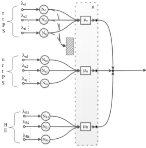
Fig. 2. Queueing model of inter-class scheduling algorithm
Therefore, the probability of ’z’ arrivals during a MAC frame can be determined by Equation 13.
P (z) = ✓
z! ◆
e z (13)
The distribution of bandwidth by the inter-class scheduling algorithm can be represented by the network diagram shown in Figure 2. The figure is based on the semantics proposed by VL Wallace and R. Rosenberg [10]. The semantic of the symbols is presented in Figure 1. In the figure, µ represents the average service rate of the uplink packet scheduler. µr, µn, and
µb denote the service rates of rtPS, nrtPS, and BE intra-class
schedulers, respectively. An approximate operation of inter-class and intra-inter-class scheduling algorithms can be logically presented by the network diagram shown in Figure 3. In the figure, µij represents the service rate observed by connection
ij.
Fig. 3. Queuing model of inter-class and intra-class scheduling algorithms
A. Analysis of BE Intra-class Scheduling Algorithm
Let us assume that there are | BE | BE connections
competing for uplink bandwidth. Connection i has an average packet arrival rate of i. The MAC frame has a length of
seconds, and #f
i is the average number of packets of
connection i served per frame. This implies that the total number of frames per second is equal to 1 and thus the average
number of packets served per second (#i) for connection i can
be given as
#i =# f
i (14)
Let Ti be the average time to serve a packet of connection
i. Then by using Equation 14, Ti can be determined as
Ti=
1 #i
=
#fi (15)
Based on equations 14 and 15, various parameters of the M/M/1 model can be determined as follow.
Scheduler utilization (⇢i) by connection i = iTi
⇢i= i
#fi
(16) The average response time (T00
i ) by the scheduler is equal
to Ti
1 ⇢i
Ti00=
#fi i
(17) The average waiting time (T0
i) for a packet of connection
i in queue is equal to ⇢iTi
Ti0=
i 2
#fi ⇣#fi i
⌘ (18)
By using Little’s formula [6], the average number of packets waiting (wi) in data queue of connection i is equal
to ⇢2 i 1 ⇢i wi = 2 i 2 #fi ⇣ #fi if ⌘ (19)
The average number of packets in the system (ri) is given
by ⇢i
1 ⇢i
ri= i
#fi i
(20) Standard deviation of ri ( ri) is equal to
p⇢ i 1 ⇢i ri= q i #fi #fi i (21) Another important parameter to determine is the probability (P ()) of packets waiting in the queue. The parameter is useful in determining the queue size for which the probability of overflow is below a given threshold P (). That is the size of queue should be to avoid overflow with a probability of P ().
P () = 1 ⇢1+i
Taking log on both sides and rearranging, we get = ln(1 P ())
ln( i
#fi )
1 (22)
B. Analysis of nrtPS Intra-class Scheduling Algorithm Let rnbe the bandwidth available for nrtPS class and %ube
the backlog of connection u at the start of current frame. The bandwidth allocated to connection u is given by Equation 12. If %uis used as basis of bandwidth distribution, then the resulting
model is very complex and demands an iterative solution. Since %uis directly proportional to u, therefore to make the analysis
simple, equation 12 can be rewritten as equation 23.
⇥u= min (%u, ↵u)+min rn, X v✏ nrtP S v !0 B B @ Xu v✏ nrtP S v 1 C C A (23) To simplify the presentation of subsequent equations we assume that ⇡u = min (%u[f ], ↵u) and ⌫u =
min rf, X v✏ nrtP S v !0 B B @ Xu v✏ nrtP S v 1 C C A. In the simplified form, equation 23 can written as
⌥u= ⇡u+ ⌫u (24)
Let lube the average packet size of connection u, then we
have Tu= lu ⇡u+ ⌫u (25) ⇢u= u lu ⇡u+ ⌫u (26) wu= ( ulu) 2 (⇡u+ ⌫u)(⇡u+ ⌫u ulu) (27) Ti0 = ul2u (⇡u+ ⌫u)(⇡u+ ⌫u ulu) (28) ru= u lu ⇡u+ ⌫u ulu (29) Ti00= lu ⇡u+ ⌫u ulu (30) ru = p (⇡u+ ⌫u) ulu ⇡u+ ⌫u ulu (31) and = ✓ ln(1 P ()) ln( ulu) ln(⇡u+ ⌫u) ◆ 1 (32)
C. Analysis of rtPS Intra-class Scheduling Algorithm
For analyzing the rtPS intra-class scheduling algorithm, a new parameter is introduced to account for the deadlines of rtPS packets. We define i be the maximum tolerable latency
of connection i. That is, if a packet k of i arrives at time ak,
then it must be scheduled between ak and ak + i to meet
the latency constraint. If the packet is not transmitted before ak+ i, then it is considered to be expired and therefore it is
dropped from the queue. The constraint of deadline makes the analysis considerably difficult than the analyses done earlier in this section.
Let | rtP S | be the number of rtPS connections and
⇥rtP S be the average bandwidth available for the rtPS class,
i.e. ⇥rtP S = X i✏ U GS[ ertP S ↵i X j✏ nrtP S ↵j BE.
The algorithm assures fairness of resource allocation by using the Equations 9 and 10. This allocation scheme implies that the average service rate of connection i can be given by Equation 33.
By using Equation 11, µi can be defined as follows µi= i ( 0) X j✏ rtP S ↵0j (33)
To make the analysis tractable, we assume that each queue can be analyzed separately with an average arrival rate of i
and average service rate of µi. Using equation 33, the values
of Ti and ⇢i can be determined as follows.
Ti= 1 µi Ti= X j✏ rtP S ↵0j i( 0) (34) Similarly, ⇢i= iTi ⇢i= X j✏ rtP S ↵0j 0 (35)
The arrival rate of each connection obeys the Poisson distribution, the average service time follows exponential dis-tribution, and the deadline is deterministic. Therefore, each rtPS queue can be analyzed as an M/M/1+D system. This class of queues were analyzed by D.Y Barrer [4]. The most important parameter for the rtPS class is maximum tolerable latency. Specifically, we are interested in knowing the number of packets dropped due to expiry of deadline. According to D.Y. Barrer, the packet loss probability (Q) under statistical equilibrium can be computed by Equation 36.
Qi =
(1 ⇢i)eµi i(⇢i 1)
1 ⇢ieµi i(⇢i 1) (36)
Since a packet is dropped if its waiting time exceeds i,
therefore T00
i is always between 0 and i, Mathematically,
0 < T00
i i. Since i is the arrival rate and Qi is the loss
probability, therefore the average packet loss rate ($i) is the
product of iand Qiand the throughput is equal to ili(1 Qi)
$i= iQi (37)
and the total packet drop rate for the entire rtPS class can be given as
$ = X
j✏ rtP S
( jQj) (38)
The average throughput (⌧i) of connection i is given by
equation 39
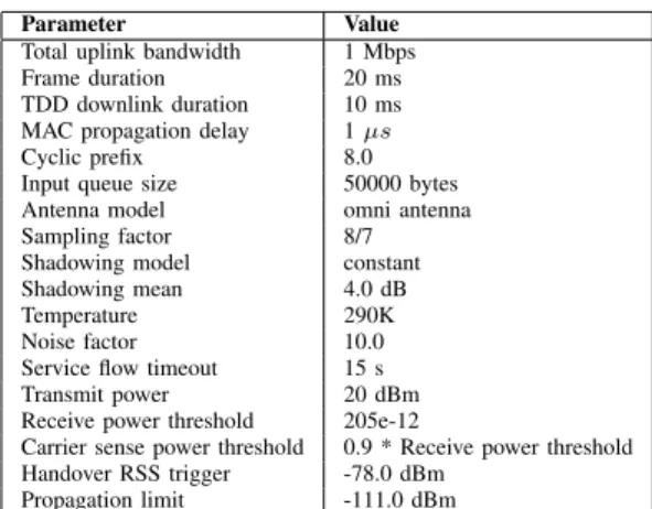
Parameter Value Total uplink bandwidth 1 Mbps Frame duration 20 ms TDD downlink duration 10 ms MAC propagation delay 1 µs Cyclic prefix 8.0 Input queue size 50000 bytes Antenna model omni antenna Sampling factor 8/7 Shadowing model constant Shadowing mean 4.0 dB Temperature 290K Noise factor 10.0 Service flow timeout 15 s Transmit power 20 dBm Receive power threshold 205e-12
Carrier sense power threshold 0.9 * Receive power threshold Handover RSS trigger -78.0 dBm
Propagation limit -111.0 dBm
TABLE I. IMPORTANT SIMULATION PARAMETERS FOR COMPARATIVE ANALYSIS
⌧i= ili(1 Qi) (39)
and the average throughput for the entire rtPS class can be determined by Equation 40.
= X
j✏ rtP S
jlj(1 Qj) (40)
The probability that the average queue size is equal to packets at statistical equilibrium can be determined by Equation 41. Pi() = iPi(0) Y j=1 (µi+ Ci(j)) 1 (41) Where, Pi(0) = 1 µiTi+ 1 and Ci(j) = µi(µi i) j 1eµi i Rµi i 0 tj 1e tdt
IV. RESULTS ANDDISCUSSION
Simulations were performed to assess the validity of the analytical model presented in Section III. The simulations of TLSA were performed in Qualnet 5.0 [9]. Qualnet is a commercial simulator developed by Scalable Network Tech-nologies (SNT). It is a suite of tools to model large scale networks. The advantage of using Qualnet is that it provides a validated and faithful simulation model of the real world IEEE 802.16 networks.
The values of important simulation parameters are shown in Table I. Each experiment was repeated 50 times and the mean value is used for the comparative study. A unique pseudo-random seed was used for each repetition to alter the characteristics of simulation such as traffic generation patterns, interference levels, back-off timers and mobility patterns.
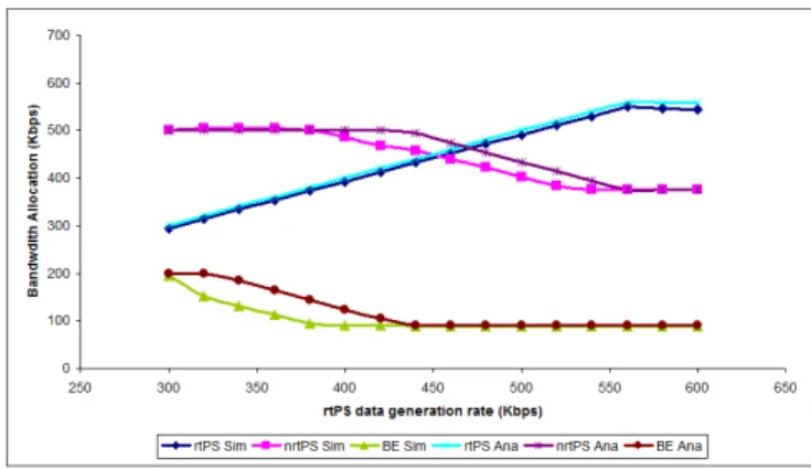
Fig. 4. Comparative analysis of inter-class bandwidth allocation
Fig. 5. Comparative analysis of packet lost in inter-class scheduling
A. Bandwidth Distribution by Inter-Class Scheduling Algo-rithm
The experiment was performed to compare the analytical and simulation models of inter-class scheduling algorithm. In this experiment, BE traffic was generated at an average rate of 200 Kbps. The value of BE was set to 90 Kbps. The
MRTR and average traffic rate of nrtPS class were 375 Kbps and 500 Kbps, respectively. The experiment was performed with increasing load of rtPS traffic. Initially rtPS traffic was generated at an average rate of 300 Kbps, which was gradually increased to 600 Kbps.
The minimum traffic rate of rtPS traffic was set to 300 Kbps, while the maximum tolerable latency was set to 160ms. Figure 4 presents the comparison of bandwidth distribution by the analytical and simulation models. For rtPS class, the average difference between simulation and analytical results is 8.34 Kbps with a standard deviation of 2.49 Kbps.
The simulation and analytical curves of nrtPS class follow the same trend. The average difference is 12.65 Kbps with a standard deviation of 16.27 Kbps. The analytical and simu-lation curves of BE class show greater differences at lower rtPS traffic rates. However, the curves converge and become identical at rtPS traffic rate of 440 Kbps and greater. The average difference between the curves is 16.69 Kbps with a standard deviation of 21.25 Kbps.
The comparative analysis of percentage of lost packets are shown in Figure 5. Initially both curves follow exactly the
Fig. 6. Comparative analysis of nrtPS intra-class scheduling
Connection MRTR (Kbps) Average Traffic Rate (Kbps) n1 140 200
n2 200 225 n3 225 275 n4 250 300 Total 815 1000
TABLE II. INPUT TRAFFIC PARAMETERS FOR COMPARATIVE ANALYSIS OF NRTPSINTRA-CLASS SCHEDULING ALGORITHM
same trend. However, deviation of the analytical curve from the simulation curve can be seen at rtPS traffic rate greater than 460 Kbps. The average difference between the curves is 0.93 percent point (pp) with a standard deviation of 1.14pp.
The comparative study suggests that the analytical model predicts the behavior of inter-class scheduling algorithm with good accuracy. Therefore, it could be concluded that the model faithfully captures the working of inter-class scheduling algorithm.
B. Intra-Class Scheduling Algorithms
1) nrtPS Class: The comparison of analytical and simula-tion models of nrtPS intra-class scheduling algorithm is shown in Figure 6. For the comparison four nrtPS connections, with parameters as shown in Table II, were used. The figure reveals that the simulation results closely matches the analytical re-sults. The average difference is 1.09 Kbps with an standard deviation of 2.42 Kbps.
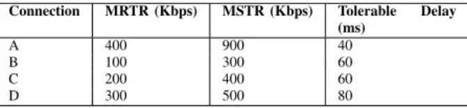
Connection MRTR (Kbps) MSTR (Kbps) Tolerable Delay (ms) A 400 900 40 B 100 300 60 C 200 400 60 D 300 500 80
TABLE III. INPUT TRAFFIC PARAMETERS FOR COMPARATIVE ANALYSIS OF RTPSINTRA-CLASS SCHEDULING ALGORITHM
Fig. 8. Comparative analysis of rtPS intra-class scheduling
2) BE Class: The comparison of analytical and simulation models of BE intra-class bandwidth allocation is shown in Figure 7. In this experiment, four SS with one BE connection each were used. The average traffic rate of connections BE1, BE2, BE3, and BE4 were 200 Kbps, 225 Kbps, 275 Kbps, and 300 Kbps, respectively. The average difference between simulation and analytical results is 9.83 Kbps with a standard deviation of 12.14 Kbps, and therefore the models are in good agreement with each other.
3) rtPS Class: The comparison of simulation and analytical results of rtPS intra-class bandwidth allocation and associated service ratios are presented in Figures 8 and 9, respectively. In this experiment, four rtPS connections, with transmission characteristics as shown in Table III, were used. The average bandwidth allocation difference between two models is 35 Kbps with a standard deviation of 17 Kbps.
The comparative analysis provided in this section reveals that the working of inter-class and intra-class scheduling algorithms is modeled with good accuracy by the proposed
Fig. 9. Comparison of connection service ratios
analytical model. The simulation results are in accordance with the analytical model and thus validates its accuracy.
V. CONCLUSION
In this paper, we presented a Markov chain based analyt-ical model of Two Level Scheduling Algorithm (TLSA) for WiMAX networks. In TLSA an inter-class scheduling algo-rithm distributes bandwidth among various WiMAX service classes, while intra-class bandwidth distribution for each class is done by a class-specific scheduling algorithm. The analyses provide detailed models of both inter-class and various intra-class scheduling algorithms. The performance study allows one to understand and analyze TLSA and the simulation results reveal that the model correctly depicts the operations of TLSA. Therefore, it can be used to predict the behavior of TLSA with good accuracy as shown in section IV.
REFERENCES
[1] Zeeshan Ahmed. Quality of Service in WiMAX for Multimedia Services. PhD thesis, Universite de Nantes France, 2013.
[2] Zeeshan Ahmed and Salima Hamma. Efficient and fair scheduling of rtPS traffic in IEEE 802.16 point-to-multipoint networks. In 4th Joint IFIP/IEEE wireless and mobile networking conferece, Oct. 2011. [3] Zeeshan Ahmed and Salima Hamma. Two-level scheduling algorithm
for different classes of traffic in WiMAX networks. In Performance Evaluation of Computer and Telecommunication Systems (SPECTS), 2012 International Symposium on, pages 1–7. IEEE, 2012.
[4] DY Barrer. Queuing with impatient customers and indifferent clerks. Operations Research, 5(5):644–649, 1957.
[5] S.A. Filin, S.N. Moiseev, M.S. Kondakov, A.V. Garmonov, Do Hyon Yim, Jaeho Lee, Sunny Chang, and Yun Sang Park. QoS-Guaranteed Cross-Layer Transmission Algorithms with Adaptive Frequency Sub-channels Allocation in the IEEE 802.16 OFDMA System. In Communi-cations, 2006. ICC ’06. IEEE International Conference on, volume 11, pages 5103 –5110, june 2006.
[6] BV (Boris Vladimirovich) Gnedenko and IN Kovalenko. Introduction to queueing theory. Birkhauser, 1989.
[7] IEEE 802.16e. IEEE 802.16-2005, IEEE standard for local and metropolitan area networks - Part 16: Air interface for fixed and mobile broadband wireless access systems amendment for physical and medium access control layers for combined fixed and mobile operation in licensed bands, February 2006.
[8] Lidong Lin, Weijia Jia, and Wenyan Lu. Performance Analysis of IEEE 802.16 Multicast and Broadcast Polling based Bandwidth Request. In Wireless Communications and Networking Conference, 2007.WCNC 2007. IEEE, pages 1854 –1859, march 2007.
[9] Qualnet simulator (version 5.02) http://web.scalable-networks.com/content/qualnet.
[10] Victor L Wallace and Richard S Rosenberg. Markovian models and numerical analysis of computer system behavior. In Proceedings of the April 26-28, 1966, Spring joint computer conference, pages 141–148. ACM, 1966.