Structure et dynamique de l'interface entre des tubes de flux entrelacés observés à la magnétopause terrestre par la mission MMS

THÈSE

THÈSE

En vue de l’obtention du

DOCTORAT DE L’UNIVERSITÉ DE TOULOUSE

Délivré par : l’Université Toulouse 3 Paul Sabatier (UT3 Paul Sabatier)

Présentée et soutenue le 11/10/2018 par :

Issaad KACEM

Structure et dynamique de l’interface entre des tubes de flux

entrelacés observés à la magnétopause terrestre par la mission MMS

JURY

SÉBASTIENGALTIER Rapporteur

ROCHSMETS Rapporteur

GENEVIÈVESOUCAIL Examinateur KARINEISSAUTIER Examinateur MATTHIEU

KRETZSCHMAR

Examinateur CHRISTIANJACQUEY Directeur de thèse VINCENTGÉNOT Co-directeur de thèse

École doctorale et spécialité :

SDU2E : Astrophysique, Sciences de l’Espace, Planétologie Unité de Recherche :

Institut de Recherche en Astrophysique et Planétologie (UMR 5277) Directeur(s) de Thèse :

Christian JACQUEY et Vincent GENOT Rapporteurs :

S

TRUCTURE AND DYNAMICS OF THE

INTERFACE BETWEEN INTERL ACING FLUX

TUBES OBSERVED AT THE

E

ARTH

’

S

MAGNETOPAUSE BY

MMS

MISSION

by

Issaad Kacem

A thesis submitted to Paul Sabatier University

for the degree of Doctor of Philosophy

defended on Thursday October 11, 2018 at 14:00 PM.

Supervisor:

Christian JACQUEY

co-Supervisor:

Vincent GENOT

Thesis committee: Sébastien GALTIER,

LPP

Roch SMETS,

LPP

Geneviève SOUCAIL,

IRAP

Karine ISSAUTIER,

LESIA

Matthieu KRETZSCHMAR, LPC2E

Olivier LECONTEL,

LPP

An electronic version of this thesis is available at

"The plain fact is that the planet does not need more successful people. But it does desperately need more peacemakers, healers, restorers, storytellers, and lovers of every kind. It needs people who live well in their places. It needs people of moral courage willing to join the fight to make the world habitable and humane. And these qualities have little to do with success as we have defined it."

David W. Orr

C

ONTENTS

List of Figures v

List of Tables xiii

Acknowledgements xv

Abstract xix

Résumé xxi

Introduction Générale xxiii

1 Introduction 1

1.1 Physics of collisionless plasmas. . . 1

1.1.1 Solar and astrophysical plasmas . . . 1

1.1.2 Collisionless plasmas properties. . . 2

1.1.3 Kinetic and fluid description . . . 8

1.1.4 Frozen-in magnetic field condition . . . 9

1.2 Magnetic reconnection in collisionless plasmas. . . 10

1.2.1 The principle of magnetic reconnection . . . 11

1.2.2 Differential ion-electron motion: Hall fields and currents. . . 12

1.2.3 Anomalous resistivity model for magnetic reconnection . . . 15

1.2.4 Reconnection rate . . . 15

1.2.5 Energy conversion rate. . . 16

1.2.6 Observational constraints for magnetic reconnection analysis. . . 17

1.3 The Earth’s magnetosphere . . . 18

1.3.1 Large-scale structure of the Earth’s magnetosphere . . . 18

1.4 Magnetic reconnection at the Earth’s magnetopause. . . 24

1.4.1 The dayside magnetopause and the boundary layer . . . 24

1.4.2 Flux transfer events. . . 25

1.4.3 FTEs characteristics . . . 26

1.5 Wave-Plasma interactions. . . 27

1.5.1 Linear plasma wave theory . . . 29

1.6 Overview of the thesis . . . 32

2 Instrumentation and analysis techniques 33 2.1 The Magnetospheric Multiscale mission (MMS). . . 33

2.2 Mission and measurements requirements . . . 33

2.3 Mission operations . . . 36

2.4 Instrument descriptions . . . 37

2.4.1 Hot Plasma Suite . . . 37

2.4.2 Energetic Particles Detector Suite . . . 42

2.4.3 Fields Suite. . . 43

2.4.4 Electron drift instrument (EDI). . . 45

2.4.5 Two Active Spacecraft Potential Control Devices (ASPOC) . . . 45

2.5 Data analysis techniques. . . 46

2.5.1 Magnetopause model . . . 46

2.5.2 Magnetopause transition parameter . . . 48

2.5.3 Curlometer technique . . . 49

2.5.4 Variance analysis: current density measurements . . . 51

2.5.5 Multi-Spacecraft Timing Analysis: structures orientation and motion . 53 2.5.6 Walén test . . . 54

2.6 Spectral analysis. . . 57

2.7 Analysis method for Lower Hybrid Drift Waves (LHDWs) . . . 58

2.8 WHAMP simulations . . . 60

3 Magnetic reconnection at a thin current sheet separating two interlaced flux tubes near the Earth’s magnetopause 61 3.1 Introduction . . . 61

3.2 Instrumentation and data . . . 62

3.3 Spacecraft location and configuration. . . 63

3.4 Solar wind observations . . . 65

3.4.1 Expected location of the reconnection sites [Trattner et al. (2007)] . . . 69

3.5 Large time-scale observations. . . 70

3.5.1 Boundary layer structure . . . 70

3.5.2 Magnetopause transition parameter . . . 75

3.6 Analysis of the event . . . 76

3.6.1 Observations. . . 76

3.6.2 Small-scale current sheet . . . 83

3.7 Discussion and interpretation . . . 89

3.7.1 Phenomenological interpretation . . . 89

3.7.2 Possible reconnection at the thin current sheet. . . 93

3.8 Summary and conclusion . . . 97

4 Plasma waves study for the event of 7 November 2015 99 4.1 Introduction . . . 99

4.2 Instrumentation. . . 99

4.3 Main features observed around the current sheet. . . 100

4.4 Plasma waves. . . 100

4.4.1 Whistler waves. . . 100

4.4.2 Lower Hybrid Drift Waves (LHDWs). . . 107

4.5 Discussion . . . 114

4.6 Summary and conclusions. . . 116

5 Summary and conclusions 117 5.1 Summary of results . . . 117

5.2 Outlook on possible developments . . . 120

5.3 A wider perspective on this work. . . 121

A Résumé et conclusions 123 A.1 Résumé des résultats . . . 123

A.2 Perspectives sur les développements possibles . . . 125 A.3 Perspectives plus larges . . . 127

L

IST OF

F

IGURES

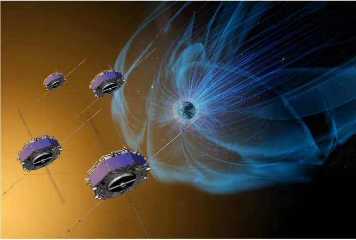
1 Artist concept of the Magnetospheric Multiscale (MMS) mission to study mag-netic reconnection. Credits: NASA. . . xxvi 1.1 Examples of plasmas.. . . 2 1.2 The ranges of temperature and densities of plasmas (1eV ∼ 11600K ). Figure

from Peratt (1996). . . 3 1.3 Electron trajectory in a uniform magnetic field. The magnetic field lines are

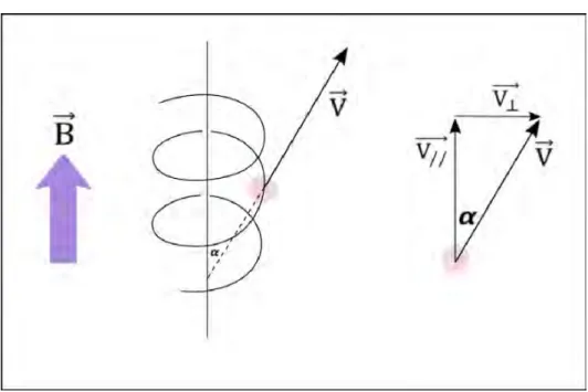
shown as straight purple arrows. . . 6 1.4 The definition of the pitch angleα for a particle gyrating around the magnetic

field lines. . . 6 1.5 Ions motion in the presence of a density gradient. More ions are moving

downwards than upwards giving rise to a drift velocity perpendicular to the magnetic field and to the density gradient. . . 7 1.6 A 2-D schematic view of the magnetic reconnection process. (a) Two opposite

magnetic field (blue and green) from different plasma regimes, are encoun-tering each other. The field lines are separated by a thin current sheet which is shown in pink, the inflow plasma from both side (purple arrows) stream into the current sheet, (b) The magnetic fields are strongly pushed towards each other, (c) a diffusion region is formed (black box) where the two magnetic fields create an X-line configuration and (d) these fields can cross the current sheet by merging into a pair of kinked lines, which will be carried away as the magnetic tension acts to straighten them. The yellow arrows represent the outflow plasma jets. The big circles represent ions while the small circles represent electrons. . . 13

1.7 Two-dimensional reconnection topology. The pink (green) box ofδi (δe) is

the ion (electron) diffusion region. The black lines show the magnetic field lines. The dashed black lines are the separatrices. The blue arrows show the plasma flow outside the diffusion region. Ions are decoupled from the magnetic field in the ion diffusion region, creating the Hall magnetic (yellow and violet quadripolar structure) and electric field patterns (magenta arrows). The ion flow is shown by dashed green arrows. The electrons remain magne-tized in the ion diffusion region and they follow the trajectories shown by red arrows. Electrons are demagnetized in the electron diffusion region.. . . 14 1.8 Zoom around the diffusion region shown in Figure 1.6-(d). The field line

dif-fuses over the half-width of the diffusion layer,δ, which is much smaller than the system size, 2L. . . . 16 1.9 A schematic view of the spiral Parker structure in the equatorial plane and

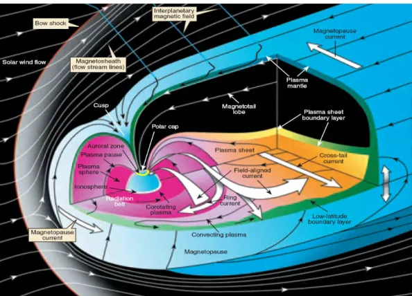
orbit of the Earth in 1 AU, showing the interplanetary magnetic field (IMF) lines frozen into a radial solar wind with an expansion at speed of 400 kms−1. As the plasma passes Earth’s orbit moving parallel to the Sun-Earth line, the IMF typically creates an angle of 45°. (Sun and Earth are not to scale). . . 19 1.10 Three-dimensional cutaway view of the Earth Magnetosphere showing

cur-rents (white arrows), fields and plasma regions. This figure is from Pollock et al. (2003). . . 21 1.11 Observations from MMS 1 on 1 December 2017 between 10:00 and 16:00 UT

while the spacecraft were moving from the magnetosphere to the solar wind. (a) the magnetic field components and intensity, (b) the ion density, (c) the ion velocity components, (d) ion spectrogram and (e) electron spectrogram. . 22 1.12 The schematic figure of plasma flow through the magnetosphere driven by

magnetic reconnection. The numbered field lines show the evolution of a field line involved in the Dungey cycle. Figure from Kivelson et al. (1995).. . . 23 1.13 Interior structure of magnetic field lines in a flux rope. Figure from Russell

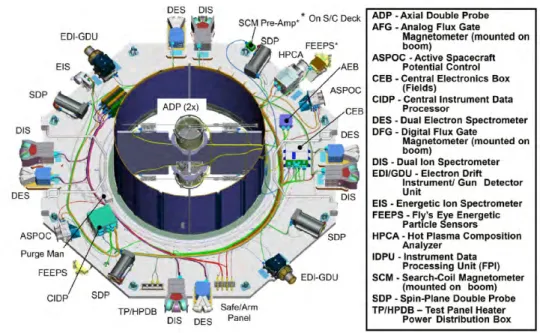
and Elphic (1978).. . . 26 2.1 Instruments onboard each MMS spacecraft. Figure from Burch et al. (2016). . 34

2.2 MMS orbital geometry and science Regions of Interest (ROI). Figure from Too-ley et al. (2016). . . 35 2.3 Schematic of the MMS formation as a science instrument concept (image

credit: NASA). . . 35 2.4 Ecliptic-plane sketch of MMS orbit. The region of interest is shown in blue

and burst data intervals are shown in red. Figure from Burch et al. (2016). . . 37 2.5 Polar angle FOV configuration of each top hat plasma spectrometer. The

spacecraft +Z axis is also indicated. Figure from Pollock et al. (2016). . . . 39 2.6 DES detection system. Figure from Pollock et al. (2016) . . . 39 2.7 (Left) Azimuthal FOV configuration of the eight spectrometers for each species

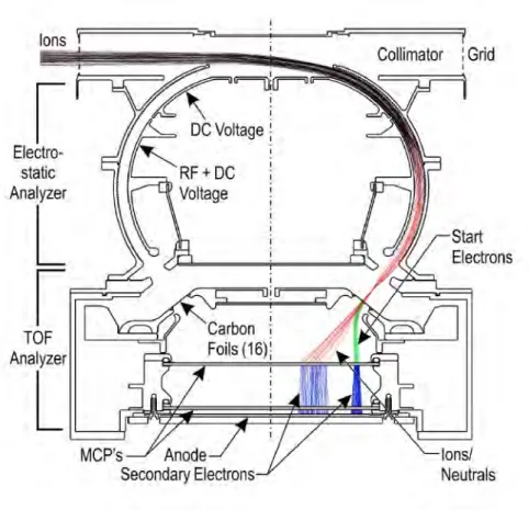
Each spectrometer, exercising four deflected fields of view, yields 32 azimuth samples for each species. (Right) The azimuth zones for each DES (DIS). Fig-ure from Pollock et al. (2016) . . . 40 2.8 Schematic drawing of the HPCA sensor together with characteristic ion and

electron trajectories. Figure from Young et al. (2016). . . 42 2.9 Magnetopause location and shape on 7 November 2015 using Shue model. . 47 2.10 Boundary coordinate system. N points outward to the local magnetopause,

L is the projection of the Earth’s magnetic dipole field and the M completes

the right-handed set, pointing dawnward (M = N × L). . . . 48 2.11 A scatter plot of the perpendicular electron temperature against the electron

density. A fourth order polynomial curve was fitted to the points. Theτ pa-rameter for each particular point is obtained by projecting it into the near-est point of the fitting curve as shown by the red line. Then, we evaluate the length of the curve between its beginning and the projected point as illus-trated by the green curve. . . 50 2.12 Illustration of the average current density estimation using the curlometer

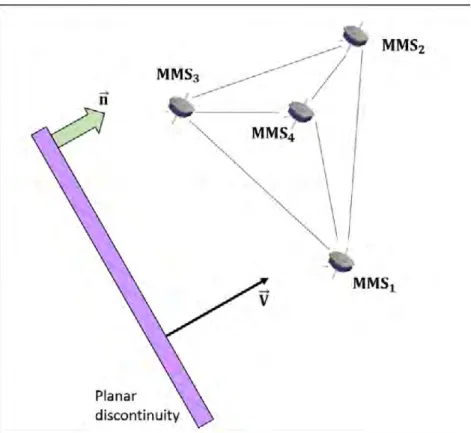
technique . . . 51 2.13 Sketch of a planar discontinuity moving at a constant velocity V toward four

2.14 (a) deHoffmann Teller analysis: the convection electric field Ec(= −V × B) vs.

the de-HT frame electric field EH T(= −VH T×B ) and a linear regression fit, (b)

Walen analysis: V0(i )vs. Vi_A of all three components and a linear regression fit. Blue, green, and red dots denote x, y, and z components in the GSE frame. Figure from Phan et al. (2013). . . 56

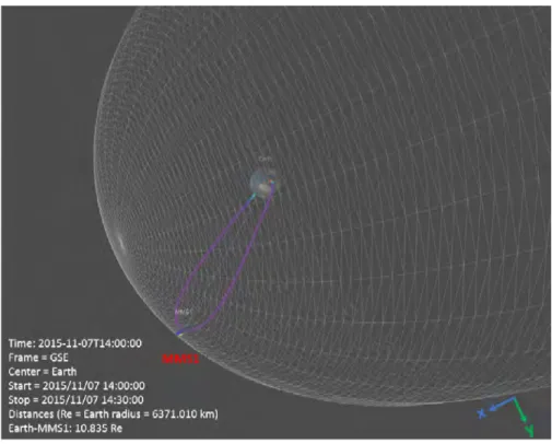
3.1 GSE equatorial-plane projection of the MMS orbit on November 7, 2015 and the normal to the magnetopause (green arrow) corresponding to the space-craft location in the ecliptic plane. The event presented in this study occurred between 14:16:05 and 14:17:20 UT. The red line corresponds to the crossing of a boundary layer. The large blue diamond shows the position at 14:15:00 UT. The probable magnetopause is indicated by green line and shaded boundaries. 64 3.2 MMS orbit on November 7, 2015 in the XZ plane at 14:00:00 UT. The large

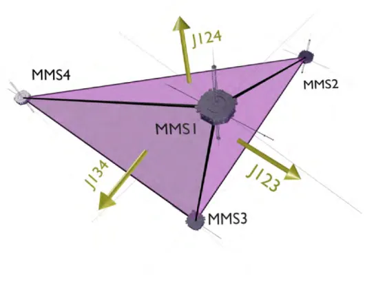
diamond is the approximate location of the spacecraft. The magnetic field lines are plotted in purple and are calculated using the Tsyganenko model [Tsyganenko and Stern (1996)]. . . 65 3.3 Configuration of the MMS tetrahedron at 09:30:54 UT on November 7, 2015.

TQF is the tetrahedron quality factor, which compares the actual tetrahedron to a regular tetrahedron [Fuselier et al. (2016)].. . . 66 3.4 Solar wind conditions from the OMNI 1 minute resolution database from

06 November 2015-00:00 UT through 09 November 2015-12:00 UT. (a) Inter-planetary magnetic field components and amplitude in GSE coordinates, (b) plasma temperature, (c) plasma density, (d) plasmaβ parameter, and (e) dis-turbance storm time (DST) index. . . 67 3.5 Solar wind conditions from the OMNI 1 minute resolution database from 06

November 2015-00:00 UT through 09 November 2015-12:00 UT. (a) Interplan-etary magnetic field components and amplitude in GSE coordinates, (b) Dis-turbance Storm Time index. Solar wind conditions during 08:00-20:00 UT on 7 November 2015, (c) Interplanetary magnetic field components in GSE coordinates, (d) solar wind dynamic dynamic pressure, and (e) Alfvén Mach number. . . 68

3.6 The magnetopause shear angle seen from the Sun with the predicted recon-nection and MMS locations at the magnetopause. Courtesy from K.J. Trattner. 71 3.7 Survey data from MMS1 on 7 November 2015 between 13:00 and 15:00 UT. (a)

Magnetic field from FGM, (b) electron and ion densities, (c) ion velocity, (d) electron spectrogram provided by FPI, (e) ion spectrogram provided by FPI, (f ) He2+spectrograms from HPCA and (g) O+spectrogram from HPCA.. . . . 72 3.8 The varitations of Bz as a function of By during the time of the LLBL

cross-ing with the logarithmic of the ratio of electron density over perpendicular electron temperature is represented by the colors of the dots on November 7, 2015 between 13:00 and 15:00 UT. . . 73 3.9 The XGSE component of the spacecraft position on November 7, 2015

be-tween 13:00 and 15:00 UT Earth Radii. The vertical dashed lines delimit the boundary layer. . . 74 3.10 Transition parameter calculated for MMS1 calculated from FPI measurements. 76 3.11 An overview of MMS1 observations between 14:15:45 and 14:17:20 UT in GSE

coordinates on 7 November 2015. (a) Magnetic field components and total field strength, (b) pressures (red= plasma (ion),green= magnetic, and black= total), (c) current density from curlometer technique, (d) ion velocity compo-nents, (e) electron (black) and ion (red) densities. The black vertical dashed lines labelled T0 to T5, correspond to times 14:16:04; 14:16:25; 14:16:40; 14:16:43; 14:16:58 and 14:17:05 UT. . . 78 3.12 MMS1 data between 14:15:45 and 14:17:20 UT of (a) Byand the magnetic field

strength in GSE coordinates, (b) electron energy spectrum. Electron pitch angle distribution in the range of (c) 98-127 eV, (d) 451-751 eV, and (e) 3304-11551 eV. . . 79 3.13 (a) Magnetic field magnitude, (b)-(d) magnetic field components in the

mag-netopause LMN frame, (e) angleΨ between the magnetopause normal and the magnetic field, (f )-(h) ion velocity components in the magnetopause LMN frame, (i) parallel (black) and perpendicular (red) ion velocity in the GSE co-ordinates system. The black vertical dashed lines labelled T0to T5are shown

3.14 By component of the magnetic field in the GSE coordinates system from the

four MMS spacecraft. The horizontal dashed lines represents the several con-tours of different Byvalues that were used to calculate their normal directions

and propagation velocities. . . 84 3.15 The relative orientation of the PCS frame (UP, UJ and UV) to the GSE frame.

The thick violet arrow shows the direction of the current sheet propagation velocity obtained from multi-spacecraft data analysis. The PCS frame corre-sponds to a translation of the GSE frame in the direction of the current sheet propagation velocity combined with a rotation about the YGSEdirection. . . 84

3.16 Current density obtained from curlometer technique on 7 November 2015 between 14:16:35 and 14:16:50 UT. (a) in GSE coordinates, (b) in the current principal axis frame. . . 85 3.17 Data from MMS1 between 14:16:38 and 14:16:44 UT (a) current density

com-ponents in the GSE coordinates system, (b) parallel, perpendicular and the total current densities, (c) electrons and ions current densities as well as the current density obtained from the curlometer technique and the current den-sity obtained from ne(Vi− Ve), (d) current density components in the PCS

frame (obtained from the curlometer technique), (e) magnetic field compo-nents in the PCS frame, (f ) ion velocity compocompo-nents in the PCS frame, (g) ion velocity components in the PCS frame between 14:16:05 and 14:17:20 UT. . . 87 3.18 A schematic view of the crossing of the current structure in the PCS frame.

The orange, green and magenta arrows show the magnetic field orientation in the F TA, current structure and F TB respectively. The black arrows in the

UJ (UV) direction correspond to the main (bipolar) current density. The two

oppositely directed red arrows in the UP direction illustrate the compression

of the current structure. The red arrows with yellow edges show the ion jet ob-served in the current structure. The spacecraft trajectory across the structure is represented by the dashed black arrow. . . 92 3.19 (a) Ion density,(b) Ion skin depth between and (c) the protons Larmor radius

3.20 Between 14:16:38 and 14:16:44 UT: (a) B data, (b) FPI currents, (c,d,e) com-parison between EDP electric field data (black), −Ve× B (green) and −Vi× B

(red). . . 95 3.21 Between 14:16:38 and 14:16:44 UT: (a) B data, (b) current density qn(Vi−

Ve) obtained from the computed moments of ion and electron distribution

functions, (c) ion velocity, (d) to (g) J ×E’ for MMS1, MMS2, MMS3 and MMS4. 96

4.1 Between 14:16:38 and 14:16:44 UT: (a) B data, (b) FPI currents, (c,d,e) com-parison between EDP electric field data (black), −Ve× B (green) and −Vi× B

(red), (f ) ion velocity,(g) parallel and perpendicular electron temperatures and (h) electron density. . . 101 4.2 MMS1 observations on 7 November 2015 between 14:16:36 and 14:16:46 UT:

(a) magnetic field components and amplitude, (b,c) band-pass filtered be-tween 256 and 512 Hz EDP and SCM waveforms in MFA (d, e) omnidirectional E and B PSD,(f ) waveangle and (g) Ellipticity. . . 102 4.3 (a) magnetic field components and amplitude in GSE coordinates, (b) to (d)

the components of Poynting flux of electromagnetic fields. . . 103 4.4 Waveforms of the first Whistler wave packet between 14:16:40.5 and 14:16:40.9

UT in GSE coordinates. (a) the magnetic field components, (b) the magnetic field filtered between 40 and 100 Hz, (c) the electric field components and (d) parallel electric field calculated by using the EDP data and the survey mag-netic field and its associated error bars (pink shading). . . 104 4.5 Zoom on the first Whistler wave packet between 14:16:40.72 and 14:16:40.76

UT (yellow shaded area in Figure 4.4). Panels are similar to 4.4. . . 105 4.6 Waveforms of the first Whistler wave packet between 14:16:41.75 and 14:16:41.90

UT. Same legends as Figure 4.4. . . 106 4.7 Electron pitch angle distributions averaged between 14:16:41.226-14:16:41.496

UT. Parallel (0°), perpendicular (90°), and anti-parallel (180°) phase space den-sities are represented by blue, green, and red traces, respectively. . . 107

4.8 Waveforms of the lower hybrid drift waves in MFA. (a) BX, BY and BZ, (b) the

magnetic field filtered between 40 and 100 Hz, (c) electron density from the four spacecraft and (d-g) parallel and perpendicular electric field also filtered between 40 and 100 Hz for MMS1, MMS2, MMS3 and MMS4, respectively. . . 109 4.9 Ion diamagnetic velocity obtained from (a) equation 4.3 and (b) equation 4.2. 111 4.10 Electric drift speed (E × B)/B2).. . . 111 4.11 (a) Electron and (b) ion perpendicular velocities in GSE coordinates from FPI. 112 4.12 The y component of: electron diamagnetic current density (blue), ion

dia-magnetic current density obtained as jd i aI = enVdi 1 (green), perpendicular current densities obtained from FPI (red), perpendicular current densities obtained from the curlometer technique (purple) and ion diamagnetic cur-rent density obtained from equation jd i aI2= enVdi 2 (yellow). . . 113 4.13 Parallel (a) and perpendicular (b) current densities obtained from the

cur-lometer technique, the particle, the ions (enV_{∥(⊥,i )}) and the electrons current densities (−enV∥(⊥,e)). . . 114

4.14 Sketch of a reconnection site. At the top, different kinds of wave spectra com-monly observed near reconnection sites are sketched. The common places to observe those waves are marked in different gray shadowing. Typical electron distribution functions in the vicinity of the separatrix are indicated as well. Figure from Vaivads et al. (2006). LHD = Lower Hybrid Drift, W = Whistler, ESW = Electrostatic solitary waves and L/UH = Langmuir/upper-hybrid waves.115

L

IST OF

T

ABLES

2.1 Top level burst-mode parameters. Table from Burch et al. (2016).. . . 37 2.2 The suggested values ofτ for the magnetosheath, the outer boundary layer,

the inner boundary layer and the magnetosphere. . . 49

3.1 The instruments that were used for this study along with their corresponding resolution in Survey and Burst modes.. . . 63 3.2 Average positions of THB, THC, Wind and Ace in REbetween 11h00 and 15h00

UT in GSE coordinates.. . . 68 3.3 Local magnetopause coordinate system obtained from the minimum

vari-ance analysis of the magnetic field.λL/λM = 5.75, λL/λN = 18.64 and λM/λN =

3.23. . . 77 3.4 Local magnetopause coordinate system obtained from the minimum

vari-ance analysis of the magnetic field.λL/λM = 5.75, λL/λN = 18.64 and λM/λN =

3.23. . . 83 3.5 The normal directions and the velocities of the propagating structure

ob-tained by performing the timing method for multiple values of By. Mean

value are:V = 66.88km/s and Nc = [−0.54, −0.03, 0.84], and the angle of each

normal vector relatively to the the X axis. . . . 85 3.6 Results of the variance analysis of the current density obtained from the

cur-lometer technique.λ1/λ2= 2.8, λ1/λ3= 43.2 and λ2/λ3= 15.43. . . 86

3.7 The unit vectors defining the PCS (Propagating Current Structure) frame.. . . 86

4.2 Properties of the LHDWs in GSE coordinates system for MMS1, MMS2, MMS3 and MMS4, respectively. Vx,Vy,Vz give the direction of propagation of the

waves, kvk gives its amplitude, f is the waves frequency, fLH is the LHDWs

frequency, λ_⊥ is the perpendicular wavelength, k_⊥ρe is the position of the

maximum growth rate of the waves, δφ/Te is the ratio between the

electro-static potential and the electron temperature and cc is the correlation coeffi-cient between the potential obtained fromδB_∥and fromδE_⊥. . . 109 4.3 Properties of the first packet of LHDWs in GSE coordinates system for MMS1,

MMS2, MMS3 and MMS4, respectively. . . 110 4.4 Properties of the second packet of LHDWs in GSE coordinates system for

A

CKNOWLEDGEMENTS

I would like to express my sincere gratitude to everyone who supported me and who’s con-tinuing to support me at every step.

First of all, I would like to thank my parents, brothers and sisters for the endless encourage-ment and the precious support they offered me throughout my life. Thank you for inspiring me to follow my dreams and for teaching me to never give up.

I am deeply indebted to the person that changed my life without even trying. Your exis-tence is what brightens my world. You mean so much to me.

I had the great chance to start my PhD only few months after the launch of the (MMS) Mag-netospheric Multiscale mission. I would like to thank the MMS operation and instrument teams as well as the science team. I would like to thank the scientists that I had the oppor-tunity to meet during workshops and especially Marit Oieroset, Charlie Farrugia, Tai Phan, Hiroshi Hasegawa, Olivier LeContel, Mitsua Oka, James Drake, Stephan Eriksson, Drew Turner, Eastwood Jonathan, Karlheinz Trattner, Daniel Graham, Stephen Fuselier, Daniel J. Gershman and Barbara Giles. I would like to thank them for the fruitful discussions we had. A special thanks to the mission PI, Jim Burch, for his encouraging and kind words. They mean a lot to me.

I take this opportunity to express my profound gratitude to Christian Jacquey, my princi-pal supervisor, for his exemplary guidance and valuable critiques throughout the course of my PhD. On a personal level, Christian inspired me by his passionate attitude. My grateful thanks are also extended to Vincent Génot, my secondary supervisor, for his valuable ad-vices throughout my research.

Besides my supervisors, I would like to thank the rest of my dissertation committee mem-bers: Geneviève Soucail, Karine Issautier, Sébastien Galtier, Roch Smets and Mathieu Kret-zschmar for their remarks and comments.

I would also like to extend my deepest gratitude to Benoit Lavraud. Thank you for being such an amazing team leader. Thank you for your kindness and benevolence. Thank you

for sharing your knowledge and time.

I wish to thank the PEPS team members, and in particular Aurélie Marchaudon, for engag-ing in remarkable scientific discussions and Emmanuel Penou who provided the "CL" data analysis and visualization software. Thanks also to Alexis Rouillard, your humor is a breath of fresh air.

I am also grateful to my collaborators. I spent one month at "Laboratoire de Physique des Plasmas" (LPP) where I had the chance to collaborate with fantastic researchers. More specifically, I would like to thank Olivier LeContel and Hugo Breuillard for their continu-ous support and for providing me the great opportunity to work on plasma waves. I also spent two months at the "Institute of Space and Astronautical Science" (ISAS/JAXA) where I have collaborated with Hiroshi Hasegawa. I would like to thank him for his great mentor-ship and guidance.

I would also like to thank the Lab director, Philippe Louarn, for his generous support. I would like to express my very great appreciation to everyone at the IRAP administration, and in particular to Dorine Roma and Josette Garcia.

A special thanks to Mina and Henda for being so attentive and caring. Nobody in the world can me laugh the way Mina does!

I would like to thank my lab mates for their continued support. Morgane, thank you for al-ways being here for me. Thank you for being such a good friend. Mikel, I think you already know it, I am so thankful for each moment we spent together, for all the shared secrets, wishes, tears, and laughter. Thank you for your friendship. I will always treasure the mem-ories we shared in my heart. I will carry them with me all the days of my life. Yoann, thank you for taking the time to listen to my problems and help me find the solutions. Thank you for showing that you care! This dissertation would not have been possible without your precious "mms tools". Sid, I am thankful to you for your contribution. You were a fantastic officemate. Thank you for providing me with a daily dose of sarcasm and for all the funny "memes" you’ve made ;) Nathanael, I think that the first thing anyone can think to thank you for is the coffee machine! But for me, you are a trustworthy and caring friend. Kévin, thank you for sharing your experience and all your advice. Mathieu, I am very happy to share MY office with you. Thanks for your time and effort helping me when I needed it. Jérémy, thank you for being the reason I met Marie ;) Thank you for your care and for the

history lessons! Baptiste, I am glad to have met you. You have a great sense of humor. Your smile spreads happiness to those around you. Michael, thank you for your continu-ous support and encouragement. It’s a pleasure to have a friend like you. I would also like to thank Edoardo, Eduardo, Mika, Margaux, Jason, Killian, Kalyani, Min-kyung, Marina, Gaëlle, Amal, Thanasis, Shirley, Rui and Illya.

Thanks to the "petits stagiaires": Ilona, Guillaume1, Nicolas, Quentin, Thibaut, Emeline, Charles, Lydia and Vincent for making my experience in IRAP exciting and fun. Pierre, thank you for the fun moments and the discussions we had in coffee breaks.

I am also grateful to Frédérique Said and Jean-François Georgis for their support in my teaching experience.

Thanks are also due to the (CNRS) "Centre National de la Recherche Scientifique", (CNES) "Centre National d’Etudes Spatiales" and "Université Paul Sabatier" for their financial sup-port.

I am also grateful to Théo. Your friendship means a lot to me.

I am grateful to my Lebanese friends who shared with me unforgettable moments and memories during my years in France ( and also in Lebanon for some of them <3 ): Hiba, Imane, Maya, Riham, Sabine, Sarah, Nour, Duaa, Zeina, Amani, Mirna, Nour, Mostafa, Joe, Tarek, Mohanad and Abed. I am very proud of you all. It’s very reassuring to have you by my side.

I also wish to thank my childhood friends Dalal, Raeda, Safaa, Khitam and Maria. I love you so much. Spending time with you always puts me in a good mood.

Special thanks to Dominique, Philippe, Damien and Daizy. You are a wonderful family. Thank you for all your support. Thank you for having faith in me. It meant so much and it still does. I also wish to thank Cléo, you cannot imagine how much I am glad I met you. I am looking forward for the trips we planned to do! Thanks also to François-Xavier and Louis-Alexandre. Your help has been invaluable to me.

Many thanks to my friends in Toulouse, Soundous, Kahina, Mehdi, Pierre, Aziz, Imane, Amira, Walid, Leila and Karim. Thank you for the beautiful moments and lovely surprises

2_{. Thank you for listening, caring and helping.}

Last but not least, I would like to express my deepest gratitude to Céline, Elisa and Nahia.

1_{Les angles sont en micro-ampères!}

I hope the best for you. I love spending time with you. Céline, you are one of the strongest woman I have ever met: Don’t ever forget that.

A

BSTRACT

Magnetic reconnection is a ubiquitous and fundamental process in space plasma physics. The MMS mission launched on 12 March 2015 was designed to provide in-situ measure-ments for analyzing the reconnection process at the Earth’s magnetosphere. In this aim, four identically instrumented spacecraft measure fields and particles in the reconnection regions with a time resolution which is one hundred times faster than previous missions. MMS allows for the first time to study the microscopic structures associated with netic reconnection and, in particular, the thin electron diffusion region. At the Earth’s mag-netopause, magnetic reconnection governs the transport of energy and momentum from the solar wind plasma into the Earth’s magnetosphere through conversion of magnetic en-ergy into kinetic and thermal energies after a rearrangement of magnetic field lines. Flux Transfer Events (FTEs) are considered to be one of the main and most typical products of magnetic reconnection at the Earth’s magnetopause. However, more complex 3D magnetic structures with signatures akin to those of FTEs might also occur at the magnetopause like interlaced flux tubes resulting from magnetic reconnection at multiple sites. The first part of the work presented in this thesis consisted of the investigation of one of these events that was observed, under unusual and extreme solar wind conditions, in the vicinity of the Earth’s magnetopause by MMS. Despite signatures that, at first glance, appeared consis-tent with a classic FTE, this event was interpreted to be the result of the interaction of two separate sets of magnetic field lines with different magnetic connectivities. The high time resolution of MMS data allowed to resolve a thin current sheet that was observed at the interface between the two sets of field lines. The current sheet was associated with a large ion jet suggesting that the current sheet was submitted to a compression which drove mag-netic reconnection and led to the formation of the ion jet. The direction, velocity and scale of different structures were inferred using multi-spacecraft data analysis techniques. This study was completed with a plasma wave analysis that focused on the reconnecting current sheet.

R

ÉSUMÉ

La reconnexion magnétique est un processus omniprésent et fondamental dans la physique des plasmas spatiaux. La "Magnetospheric multiscale mission" (MMS) de la NASA, lancée le 12 mars 2015, a été conçue pour fournir des mesures in-situ permettant d’analyser le processus de reconnexion dans la magnétosphère terrestre. Dans ce but, quatre satel-lites identiquement instrumentés mesurent les champs électromagnétiques et les partic-ules chargées dans les régions de reconnexion, avec une résolution temporelle cent fois meilleure que celle des missions précédentes. MMS permet, pour la première fois, d’étudier les structures microscopiques associées à la reconnexion magnétique et, en particulier, la région de diffusion électronique. Au niveau de la magnétopause terrestre, la reconnex-ion magnétique a un rôle chef dans le transport de l’énergie du vent solaire vers la mag-nétosphère terrestre, en convertissant l’énergie magnétique en énergie cinétique et ther-mique. Les événements à transfert de flux (FTEs) sont considérés comme l’un des produits principaux et les plus typiques de la reconnexion magnétique à la magnétopause terrestre. Cependant, des structures magnétiques 3D plus complexes, avec des signatures similaires à celles des FTEs, peuvent également exister à la magnétopause. On retrouve, par exemple, des tubes de flux entrelacés qui résultent de reconnexions magnétiques ayant eues lieu à des sites différents. La première partie de cette thèse étudie l’un de ces événements, qui a été observé dans des conditions de vent solaire inhabituelles, au voisinage de la mag-nétopause terrestre par MMS. Malgré des signatures qui, à première vue, semblaient co-hérentes avec un FTE classique, cet événement a été interprété comme étant le résultat de l’interaction de deux tubes de flux avec des connectivités magnétiques différentes. La haute résolution temporelle des données MMS a permis d’étudier en détail une fine couche de courant observée à l’interface entre les deux tubes de flux. La couche de courant était associée à un jet d’ions, suggérant ainsi que la couche de courant était soumise à une com-pression qui a entraîné une reconnexion magnétique à l’origine du jet d’ions. La direction, la vitesse de propagation et la taille de différentes structures ont été déduites en utilisant

des techniques d’analyse de données de plusieurs satellites. La deuxième partie de la thèse fournit une étude complémentaire à la précédente et s’intéresse aux ondes observées au-tour de la couche de courant.

I

NTRODUCTION

G

ÉNÉRALE

La reconnexion magnétique est l’un des processus les plus importants dans la physique des plasmas spatiaux qui se produit dans la quasi-totalité de l’Univers: dans les plasmas astrophysiques, dans l’environnement terrestre, dans les galaxies, et au niveau du Soleil également. Ce processus fondamental se déclenche lorsque des lignes de champ de di-rections opposées se rapprochent. Ce réarrangement de polarité de champ magnétique s’accompagne d’une dissipation rapide de l’énergie magnétique qui est transférée aux par-ticules chargées sous forme de chauffage et d’écoulement. Au-delà de la reconnexion mag-nétique elle-même, l’analyse et la caractérisation de ses produits (structures de courant, fronts d’injection, cordes de flux...) permettront de mieux comprendre ce processus. La reconnexion magnétique joue un rôle crucial dans les relations Soleil-Terre et dans la dynamique de la magnétosphère. Au niveau de la magnétopause, elle est le principal pro-cessus assurant le transport d’énergie du vent solaire vers la magnétosphère. Elle résulte de l’interaction entre les lignes de champ du milieu interplanétaire et celles du champ mag-nétique terrestre. Elle se produit également dans la couche de plasma de la queue magné-tosphérique.

Les événements à transfert de flux (FTEs) sont considérés comme l’un des produits prin-cipaux et les plus typiques de la reconnexion magnétique à la magnétopause terrestre. Ils sont caractérisés par un pic d’intensité du champ magnétique et une signature bipolaire sur la composante du champ magnétique normale à la magnétopause. Cependant, des structures magnétiques 3D plus complexes peuvent également exister à la magnétopause. Ce manuscrit reporte l’analyse de l’une d’entre elles observée par la mission MMS (Magne-tospheric multiscale).

Les propriétés à grande échelle de la reconnexion magnétique sont assez bien connues grâce aux missions magnétosphériques précédentes (THEMIS, CLUSTER,...), mais l’étude des mécanismes à petite échelle n’a été possible qu’avec la mission Magnetospheric Multi-scale (MMS). MMS est une mission de la NASA qui comprend quatre satellites en

configu-ration tétraédrique avec de petites distances inter-satellites (de l’ordre de 10 km à comparer avec 100 à 1000 km pour Cluster). MMS a été lancée le 12 mars 2015 et a été conçue pour fournir des mesures in-situ permettant d’analyser avec la précision nécessaire et inégalée auparavant le processus de reconnexion à la magnétopause terrestre. Les instruments à bord de MMS offrent des mesures des champs électromagnétiques et des particules, avec une résolution temporelle cent fois meilleure que celle des missions précédentes. MMS a permis d’accéder, pour la première fois, à la dynamique des électrons, alors que toutes les missions précédentes ont été limitées à observer la dynamique des ions qui a lieu sur une plus grande échelle.

Parmi les laboratoires impliqués dans la mission MMS, on compte deux laboratoires français: l’Institut de Recherche en Astrophysique et Planétologie (IRAP) à Toulouse et le Laboratoire de Physique des Plasmas (LPP) à Paris.

Ma thèse a été centrée sur l’exploitation des données fournies par MMS. Ce manuscrit se divise en cinq chapitres précédés par la présente introduction générale:

• Dans le Chapitre1, un aperçu des concepts de base de la physique des plasmas en rapport avec la thèse est présenté. Ensuite, une brève description des plasmas du système solaire est donnée, suivie d’une introduction à la reconnexion magnétique à la magnétopause puis aux événements de transfert de flux.

• La première section du Chapitre2fournit une introduction à la mission MMS avec une brève description des principaux instruments utilisés dans cette thèse. La deux-ième section présente les techniques d’analyse utilisées.

• Le Chapitre3étudie un événement qui a été observé par MMS au voisinage de la magnétopause terrestre. Une comparaison de cet événement avec les FTEs clas-siques a été effectuée. Une interprétation phénoménologique a été aussi proposée afin de mieux comprendre les observations. La structure d’une couche de courant observée au centre de l’événement ainsi que sa géométrie spécifique intéressante ont également été décrites. Ensuite, les observations de particules à haute résolution ont été utilisées, ainsi que les données de champ magnétique pour tester l’hypothèse de reconnexion au sein de la couche de courant.

• Le Chapitre4est consacré à l’étude des ondes observées au cours de l’événement discuté dans le chapitre3et en particulier autour de la couche de courant.

En conclusion, un sommaire des résultats ainsi que quelques perspectives de recherche sont énoncées et discutées dans le Chapitre5.

Figure 1 – Artist concept of the Magnetospheric Multiscale (MMS) mission to study magnetic reconnection. Credits: NASA.

1

I

NTRODUCTION

In this chapter, we will present an overview of the basic plasma physics concepts of rel-evance to the thesis. Then, a brief description of the solar system plasmas will be given, followed by an introduction to magnetic reconnection at the magnetopause then to Flux Transfer Events and to other products of magnetic reconnection.

1.1.

P

HYSICS OF COLLISIONLESS PLASMAS

1.1.1.

S

Most of the ordinary matter in the Universe is known to be made of plasma. A plasma is a globally neutral ionized gas consisting of positively and negatively charged particles that exhibits a collective behavior [Chen(1974)]. Plasmas are found throughout the Solar Sys-tem and beyond. The Earth’s magnetosphere, gaseous nebulae, the solar corona and solar wind, the tails of comets and the Van Allen radiation belts are made of plasmas. Some of the main examples of plasmas can be sorted with respect to their temperature and density as shown in Figure1.2. As seen, the electron temperature of plasmas may vary over about 7 orders of magnitude and their electron density vary over about 30 orders of magnitude.

Plasmas may be classified in different ways. We can, for example, distinguish collisional from collisionless plasmas. In a plasma, two charged particles can interact by collisions

Figure 1.1 – Examples of plasmas.

through the Coulomb force. Collisionless plasmas, as the name says, are plasmas where the collisions between particles do not play a significant role in the dynamics of the plasma. The mean free path, i.e. the mean distance a particle travels between two successive colli-sions, is larger than the typical macroscopic length scale over which plasma quantities vary. In other words, the collision frequency is much smaller than the characteristic frequencies of the medium. Collisionless conditions are quite frequent in astrophysics when the plas-mas are sufficiently diluted like found in the collisionless shocks for supernovae. Also, the solar wind and planetary magnetospheres, which are the main plasmas considered in this thesis, exclusively consist of collisionless plasmas.

1.1.2.

C

A charged particle generates an electrical Coulomb potential field. The effect of this Coulomb potential is that a particle attracts oppositely charged particles and repels like-charged par-ticles. In a plasma, there is an abundance of negatively and positively charged particles so that a cloud of oppositely charged particles forms around a charged particle. This effect is known as Debye Shielding and maintains the quasi-neutrality of a plasma on large scales.

The spatial scale over which the charge neutrality is violated is called the Debye length:

λD=

s

ε0kBTe

ne2 (1.1)

whereε0is the permittivity of free space, kB is the Boltzmann constant, Teis the electron

temperature, n is the plasma density and e is the elementary charge. The Debye lengthλD

is defined as the scale size on which the Debye shielding occurs. In a plasma, the Coulomb force extends to the Debye length. At distances larger than the Debye length (d À λD), the

potential of a single point charge diminishes exponentially due to Debye Shielding.

The quasi-neutrality of a plasma requires that the scale size of the plasma L to be much larger than the Debye lengthλD:

L À λD (1.2)

When the quasi-neutrality of a plasma is disturbed by some external forces, the particles will be accelerated by the resulting electric field. The system then tends to recover the quasi-neutrality. This results in a back and forth movement around the equilibrium posi-tion and leads to a collective oscillaposi-tion of the particles. The typical oscillaposi-tion frequency is the plasma frequency and is given by:

ωp=

s nq2

mε0

(1.3)

where n, q and m are the density, charge and mass of the considered particle. The electron plasma frequencyωpeis the most fundamental time-scale in fully ionized plasmas.

The plasma frequencyωp yields the expression for the plasma skin depth also called the

inertial length:

δ = c ωp

(1.4) where c is the speed of light.

A particle of charge q and mass m moving with a velocity v , under the presence of an elec-tric field E and a magnetic field B , is subject to the Lorentz force:

The equation of motion of a charged particle in electromagnetic fields is:

md v

d t = q(E + v × B ) (1.6)

In the presence of a uniform magnetic field, without an electric field, the component of velocity parallel to the magnetic field v_∥ remains at its initial value and the particle is ac-celerated in a direction perpendicular to v and B . The particle will have a circular motion around the magnetic field lines, with a gyrofrequency, or cyclotron frequencyωc and a

gyration radiusρL.ωc is given by:

ωc=q|B|

m (1.7)

The radius of the circular motion, centered about the magnetic field lines, is often known as gyroradius or Larmor radius and is given by:

ρL=

v_⊥ ωc

(1.8)

where v_⊥is the perpendicular velocity of the considered particle, respectively. Owing to their opposite electric charge, ions and electrons rotate in opposite directions. In addition to the perpendicular component of the velocity, particles travel with a constant velocity along the magnetic field lines. The particle’s path describes a helix as a result of the combi-nation of the parallel and perpendicular velocities (Figure1.3).

The inertial length and gyroradius are much larger for ions than for electrons since ions are much heavier. The different temporal and length scales in a plasma help to introduce a hierarchy which order the physical processes acting at the respective scales, as will be discussed in Section1.2 for the magnetic reconnection process. The angle between the particle velocity and the magnetic field is known as the pitch angleα (Figure1.4):

α = atan³v⊥ v//

´

(1.9)

Whenα = 0°, this means that the particles are moving purely along the magnetic field lines (also called field-aligned particles). Conversely, particles withα = 90° move perpendicular to the magnetic field.

in-Figure 1.3 – Electron trajectory in a uniform magnetic field. The magnetic field lines are shown as straight purple arrows.

Figure 1.5 – Ions motion in the presence of a density gradient. More ions are moving downwards than upwards giving rise to a drift velocity perpendicular to the magnetic field and to the density gradient.

stance, under the presence of a perpendicular electric field, a drift motion ,Vd, relative to

the helical orbit of the orbits is added to the particle motion:

Vd =E × B

B2 (1.10)

This velocity describes the motion of the magnetic field lines and the frozen plasma. The

E ×B drift is perpendicular to both the electric and magnetic fields. Both ions and electrons

drift in the same direction since Vd is independent of the sign of the particle charge.

Another gyrocenter drift follows from the presence of a density gradient, when more parti-cles move in the direction of ∇n × B than in the opposite direction. This effect, illustrated in Figure1.5, is called diamagnetic drift Vd i awhich is given by:

Vd i a=B × (∇ · P)

nqB2 (1.11)

where P = nT kB.

parameter known as plasma beta. The magnetic field gives rise to a magnetic pressure B2/(2µ0) which acts perpendicular to the field lines. The ratio of the thermal pressure to

the magnetic pressure defines the plasma beta:

β =pt h pB = nkBT B2_/(2µ 0) (1.12)

where T is the plasma temperature. β represents the relative importance of the forces ex-erted on the plasma by the pressure gradients and the magnetic field. In a high-beta or hot plasma, the thermal pressure dominates. Conversely, in a low-beta or cold plasma the magnetic pressure has a larger effect.

1.1.3.

K

Having discussed how individual particles behave in a plasma, it would be useful to briefly describe another plasma descriptions: the kinetic approach and the fluid approach. The kinetic approach is a statistical description of plasmas that considers the collective behav-ior and describes the system using the distribution function of the particle populations in phase space instead of solving the equation of motion for each charged particle. Each par-ticle is characterized by its 3D position xi(t ) and its 3D velocity vi(t ). The phase space

is defined by the axes (x, v ). The phase space density, f (x, v , t ), is the probability density such that f (x, v , t )d xd v is the number of particles in phase space volume element d xd v at time t . The phase space density contains considerable information regarding the phys-ical state of the plasma. This approach is widely used for the calculation of macroscopic plasma parameters, from particle distribution data derived from directional particle count rates observed by spacecraft. The macroscopic plasma parameters (e.g. density, velocity, temperature) are computed as moments of the particle velocity distributions.

The fluid approach is used for describing the macrospcopic plasma physics. In this ap-proach, the plasma is considered to be composed of two or more fluids, one for each species. Each fluid can be described by a density, temperature and bulk velocity (V ). The magne-tohydrodynamic approach (MHD) describes the plasma as a single fluid with macroscopic

variables and neglects the single particle aspects.

1.1.4.

F

-

Let us consider now a magnetized and highly conductive (i.e. η ∼ 0) plasma with charac-teristic scale and time variations which are much larger than those of particle processes. In such situation, particles always perform helical orbits around magnetic field lines (section 1.1.2). The plasma motion then follows the ideal MHD law which can be expressed as:

E = −V × B (1.13)

Whenever equation1.13holds, the plasma obeys the frozen-in-flow condition which states that the magnetic flux is conserved along the plasma flow lines. This can be noticed by combining equation1.13with Maxwell-Faraday’s Law:

∂B

∂t = −∇ × E (1.14)

to obtain the magnetic induction equation which governs the magnetic field evolution in time:

∂B

∂t = ∇ × (V × B ) (1.15)

This equation leads to the frozen-flux theorem, also known as the Alfvén’s theorem, which holds that in a perfectly conducting plasma (i.e.η = 0) the magnetic field lines behave as if they move with the plasma. In other words, the frozen-in theorem states that the magnetic flux passing through any closed surface perpendicular to the magnetic field and moving with the local plasma velocity does not vary in time:

dφ d t = Ï _³∂B ∂t − ∇ × (V × B ) ´ d S = 0 (1.16)

whereφ is the magnetic flux through a variable surface S. Considering a closed curve C bounding a surface S, the magnetic field lines which are enclosed by C define a magnetic flux tube along which the magnetic fluxφ is constant.

plasma description breaks down and more terms have to be added to the ideal MHD law. Under these conditions, ideal MHD law has to be replaced by the Ohm’s law [Baumjohann and Treumann(1996)], which in the simplest case, can be expressed as:

E + Vi× B = ηJ − 1 nee∇ · (Pe) + 1 neJ × B − me e dVe d t (1.17)

where E is the electric field and Vi× B is the induction electric field associated with the average ion motion perpendicular to the magnetic field direction. The first term on the right-hand side gives the Ohmic resistance term whereη is the resistivity. The second term represents the ambipolar electric field created by the electron density gradients in order to maintain the quasineutrality of the plasma when electrons are driven by pressure gradient. The third term expresses the Hall term. The final term expresses the effect of electron iner-tia. All the term on the right-hand of1.17are called non-ideal terms.

An important consequence of the presence these terms is that they may lead to the viola-tion of the frozen-in condiviola-tion. In other words, whenever the system develops small scale structure, one may expect the frozen-in condition to break down and the plasma dynamics to decouple from the magnetic field.

1.2.

M

AGNETIC RECONNECTION IN COLLISIONLESS PLASMAS

Magnetic reconnection is an ubiquitous energy conversion process in space plasma physics. It is expected to play key role in astrophysical phenomena. In the solar system, the mag-netic reconnection allows energy conversion in solar flares, coronal mass ejections or at the earth’s magnetopause as result of the interaction between the solar wind and the mag-netosphere magnetic field lines. Magnetic reconnection is also found in laboratory exper-iments, and particularly those about magnetic-confinement fusion. The magnetic recon-nection allows the conrecon-nection between two magnetic field lines previously independent leading to a mixing between the two plasma populations. It also leads to the conversion of magnetic energy into mechanical energy by ejecting heated plasma apart from the recon-nection site at the Alfvén speed , which can be expressed as:

VA= c ωc ωp = |B| p nmµ0 (1.18)

whereµ0is permeability of free space.

1.2.1.

T

Figure1.6shows a schematic view of the magnetic reconnection process between two op-positely directed magnetic fields separated by a current sheet (Figure1.6-(a)). Under the frozen-in condition, magnetic field and plasma from different sources can not mix. The magnetic field lines, initially straight, are pushed towards the current sheet by external forces (Figure1.6-(b)), until the frozen-in-flow assumption breaks down. The region where the frozen-in condition breaks down (i.e. that the equation1.13is not satisfied anymore) is called diffusion region. From a kinetic point of view, breaking the frozen-in condition means that particles do not simply gyrate around magnetic field lines but instead perform more complicate orbits. This behavior is possible only where the scale of the system L is smaller than the dimensions characterizing the particles’ motions, i.e. the local gyroradius ρ. The fluid manifestation of these kinetic effects is the presence of non-ideal terms in the Ohm’s law (Equation1.17). This means that inside the diffusion region, the ideal MHD Ohm’s law does not hold anymore (Equation equation1.13). In the diffusion region, the magnetic field can reconnect taking a X-shape configuration (Figure1.6-(c)). The point at the center, where the magnetic field strength equals zero, is called X-point. Here, the field lines merge and generate two kinked field lines which cross the current sheet. In 3D, the X-point becomes an X-line and lies perpendicular to the reconnection plane that drives the reconnection. The presence of an out of plane magnetic field, called guide field, changes the reconnection process. The newly merged field lines are then carried away from the diffusion region (Figure 1.6-(d)). The boundary separating the field lines which have un-dergone reconnection from those which have not is referred to as the separatrix which can be considered as rotational discontinuities.

The magnetic reconnection is also associated with energy conversion. If we consider a rect-angular diffusion region with a length of 2L and thickness of 2δ, the mass conservation law over the contour of the diffusion region can be written as:

I

In symmetric conditions, where the plasma conditions are identical on both sides of the current sheet, the mass conservation can be expressed as:

ni nVi nL = noutVoutδ (1.20)

where Vi n and ni n are the plasma velocity and density in the inflow region and Vout and

nout are the plasma velocity and density in the outflow region. Sinceδ/L ¿ 1, we can

de-duce from equation1.20that the plasma is accelerated in the diffusion region leading to plasma jets. The magnetic flux conservation can be used to determine the relation between the inflow and outflow magnetic fields and velocities:

Bi nVi n= BoutVout (1.21)

This equation illustrates the conversion of the magnetic energy into kinetic energy since an increasing of velocity between the inflow and outflow regions will be associated with a decreasing of the magnetic field in the corresponding region.

1.2.2.

D

-

: H

Magnetic reconnection is a multi-scale process. It occurs basically on three scales: • The MHD scales: L À ρi, T À ω−1_pi,

• The ion scales: L ∼ ρi, T ∼ ω−1_pi,

• The electron scales: L ∼ ρe, T ∼ ω−1pe.

Figure1.7shows more detailed 2-D schematic view of magnetic reconnection where both ions and electrons are considered. Initially, the two anti-parallel magnetic fields in the X direction are embedded in the plasma which flows with an inflow velocity Vi n = E × B or

"frozen in" velocity. When the magnetic fields reconnect, magnetic energy will be released in the form of accelerated electrons and ions that rapidly move away from the reconnection region in the Y direction (horizontal blue arrows). Since ions and electrons have signifi-cantly different gyroradii (ρi À ρe), the diffusion region develops two-scale structure: the

Figure 1.6 – A 2-D schematic view of the magnetic reconnection process. (a) Two opposite magnetic field (blue and green) from different plasma regimes, are encountering each other. The field lines are separated by a thin current sheet which is shown in pink, the inflow plasma from both side (purple arrows) stream into the current sheet, (b) The magnetic fields are strongly pushed towards each other, (c) a diffusion region is formed (black box) where the two magnetic fields create an X-line configuration and (d) these fields can cross the current sheet by merging into a pair of kinked lines, which will be carried away as the magnetic tension acts to straighten them. The yellow arrows represent the outflow plasma jets. The big circles represent ions while the small circles represent electrons.

region of size of the electron inertial lengthδe= c/ωpe (pink and green shaded regions in

Figure1.7). In the ion diffusion region, ions do not flow with a E × B velocity and are de-magnetized. The electrons remain frozen in until the electron diffusion region which is a much smaller scale region. Differential motion between unmagnetized ions and magne-tized electrons lead to the creation of Hall currents J = en(Vi− Ve) ∼ −enVein the

recon-nection plane. The Hall currents then lead to the creation of out-of-plane magnetic fields in the direction perpendicular to the current density direction. These fields are called the Hall magnetic fields. They correspond to a quadrupole pattern of the out-of-plane component of the magnetic field inside the reconnection region on the scale size of the ion diffusion region. They are represented by yellow and violet ovals in Figure1.7.

Figure 1.7 – Two-dimensional reconnection topology. The pink (green) box ofδi (δe) is the ion (electron)

diffusion region. The black lines show the magnetic field lines. The dashed black lines are the separatrices. The blue arrows show the plasma flow outside the diffusion region. Ions are decoupled from the magnetic field in the ion diffusion region, creating the Hall magnetic (yellow and violet quadripolar structure) and electric field patterns (magenta arrows). The ion flow is shown by dashed green arrows. The electrons remain magnetized in the ion diffusion region and they follow the trajectories shown by red arrows. Electrons are demagnetized in the electron diffusion region.

the ideal MHD laws (E = −Vi× B ) anymore. They now satisfy the Hall MHD law:

E = −Vi× B +J × B

en (1.22)

The term J × B/en creates an electric field perpendicular to the magnetic field (magenta arrows). This field is called the Hall electric field and points toward the central current sheet at the edge of diffusion region.

In the presence of several types of ions of different masses, multiple ion diffusion regions may exist according to the mass and temperature of each ion population.

1.2.3.

A

Two major mechanisms may produce resistivity in a plasma. The first possibility results from momentum exchange through electron collisions and corresponds to the microscopic Ohmic resistivity. The second possibility does not involve particle-particle interactions but instead consists of a momentum exchange by small-scale wave-particle processes, pos-sibly active also in collisionless plasma regimes. The resistivity resulting from this second mechanism is commonly called anomalous resistivity and is substantially larger than the microscopic Ohmic resistivity inside electron diffusion regions, for the plasmas we study throughout this work. Indeed, since strong current density in the dissipation region leads to a large relative streaming between ions and electrons, many plasma instabilities can be excited in this region, notably when the drift velocity of the current-carrying electrons ex-ceeds a certain threshold, such as the electron thermal speed. Waves excited due to in-stabilities, developing in a naturally turbulent way, provide an efficient mechanism for the scattering of electrons onto ions, ultimately leading to the anomalous resistivity.

1.2.4.

R

The reconnection rate R is the amount of magnetic flux reconnecting per unit time per unit length of the reconnection line. The reconnection rate is also defined as the ratio of the plasma flow velocities of the inflow and outflow regions as a first approximation. Consider-ing an elongated magnetic diffusion region (with length 2L and width 2δ ¿ 2L as illustrated in Figure1.8) which lies between two identical plasmas with oppositely directed magnetic

Figure 1.8 – Zoom around the diffusion region shown in Figure1.6-(d). The field line diffuses over the half-width of the diffusion layer,δ, which is much smaller than the system size, 2L.

field lines, R can be expressed as:

R ≡ Vi n Vout

(1.23) The reconnection rate is strongly linked to the geometry of the reconnection and corre-ponds to the ratio of the angular widths of the outflow to inflow regions (δ/L).

Both observations and models predicted a reconnection rate of 0.1 in normalized units over a wide range of parameters [e.g.Chen et al.(2017);Liu et al.(2018)]. However, despite mul-tiple observational and theoretical works, the physical origin of this value is still unclear [Cassak et al.(2017)]

1.2.5.

E

The temporal change of electromagnetic energy density, W , can be obtained by combining Maxwell’s equations: dW d t = ∂ ∂t ³B2 2µ0 ´ + ∇ · ³E × B µ0 ´ = −J · E (1.24)

where (E ×B)/µ0) is the Poynting flux. In a steady state, the regions where J ·E > 0 are sinks

of Poynting flux S and, conversely, regions where J · E < 0 are sources of Poynting flux. In the reconnection dissipation region, J · E is supposed to be positive because magnetic re-connection is known to be a dissipative process that converts magnetic energy into heat and kinetic energy.

1.2.6.

O

Multi-spacecraft studies have proven to be an invaluable tool to better understand the mag-netic reconnection process. The Cluster mission [Escoubet et al.(2001)] allowed the study of the magnetic reconnection and its diffusion region at the magnetopause on ion-scales. However, despite numerous studies on this subject, many aspects about magnetic recon-nection remain unclear due to the limited resolution of instruments aboard past missions. More recently, the Magnetospheric Multiscale (MMS) mission launched on March 12, 2015 was designed to better understand the magnetic reconnection process. MMS is composed by four identical satellites flying in adjustable tetrahedral formation allowing the observa-tion of the three dimensional structure of magnetic reconnecobserva-tion and the measurements of the spatial gradients of various plasma and field parameters. The MMS mission was de-signed to answer specific questions about reconnection by providing unprecedented spa-tial and time resolution measurements. MMS makes the study of microscopic structures and, in particular, of the thin electron diffusion region possible [Burch et al.(2016)]. Previous missions provided observations of relatively large regions of the magnetopshere. They allowed the study of magnetic reconnection at the MHD (e.g. ISEE, AMPTE, Geotail, Wind) and ion (Cluster) scales. The challenge of MMS was thus to extend these under-standings to the electron scale. It is at this scale that the magnetic field lines break and reconnect and that the processes leading to the dissipation process that converts magnetic energy into kinetic energy and heat occur. On electronic length scales, the plasma is de-scribed by the Ohm’s law shown in Equation1.17. This equation shows the terms that need to be considered when the frozen-in condition is broken: the resistive term, the divergence of the electron pressure tensor and by the electron inertia term. These terms introduce new physics to the system at short scales. In order to take into account these terms, the require-ments for MMS were to provide three-dimensional maps of particle distribution functions, electric and magnetic fields, and plasma waves within the electron diffusion region. At the dayside, the densities are high and the scale of the electron diffusion region is of the order of the electron skin depth, i.e. 10 km, or less. The spacecraft separation of MMS is about ∼ 10 km while it scans the dayside magnetopause. The time resolution of measurements were