Strain capacity assessment of API X65 steel using damage mechanics

(1)

HAL Id: hal-01633698

https://hal-mines-paristech.archives-ouvertes.fr/hal-01633698

Submitted on 13 Nov 2017

HAL is a multi-disciplinary open access archive for the deposit and dissemination of sci-entific research documents, whether they are pub-lished or not. The documents may come from teaching and research institutions in France or abroad, or from public or private research centers.

L’archive ouverte pluridisciplinaire HAL, est destinée au dépôt et à la diffusion de documents scientifiques de niveau recherche, publiés ou non, émanant des établissements d’enseignement et de recherche français ou étrangers, des laboratoires publics ou privés.

Strain capacity assessment of API X65 steel using

damage mechanics

Gabriel Testa, Nicola Bonora, Domenico Gentile, Andrew Ruggiero, Gianluca

Iannitti, Antonio Carlucci, Yazid Madi

To cite this version:

Gabriel Testa, Nicola Bonora, Domenico Gentile, Andrew Ruggiero, Gianluca Iannitti, et al.. Strain capacity assessment of API X65 steel using damage mechanics. Frattura ed Integrità Strutturale / Fracture and Structural Integrity, Università di Cassino, 2017, 42, pp.315-327. �10.3221/IGF-ESIS.42.33�. �hal-01633698�

(2)

G. Testa et alii, Frattura ed Integrità Strutturale, 42 (2017) 315-327; DOI: 10.3221/IGF-ESIS.42.33

315

Strain capacity assessment of API X65 steel using damage mechanics

Gabriel Testa, Nicola Bonora, Domenico Gentile, Andrew Ruggiero, Gianluca Iannitti

University of Cassino and Southern Lazio, Italy

gabriel.testa@unicas.it, http://orcid.org/0000-0001-2345-6789

Antonio Carlucci

SAIPEM SA, Italy

antonio.carlucci@saipem.com

Yazid Madi

EPF-Ecole d'ingénieurs / MINES ParisTech, France

yazid.madi@epf.fr

A

BSTRACT

.

Strain-based design for offshore pipeline requires a considerable

experimental work aimed to determine the material fracture toughness and

the effective strain capacity of pipe and welds. Continuum damage mechanics

can be used to limit the experimental effort and to perform most of the

assessment analysis and evaluation in a simulation environment. In this work,

the possibility to predict accurately fracture resistance of X65 steel using a

CDM model proposed by the authors, is shown. The procedure for material

and damage model parameters identification is presented. Damage model

predictive capability was demonstrated predicting ductile crack growth in

SENB and SENT fracture specimens.

K

EYWORDS

.

Damage mechanics; Fracture toughness; Strain capacity;

Strain-based design.

Citation: Testa, G., Bonora, N., Gentile, D.,

Ruggiero, A., Iannitti, G., Carlucci, A., Madi, Y., Strain capacity assessment of API X65 steel using damage mechanics, Frattura ed Integrità Strutturale, 42 (2017) 315-327.

Received: 25.07.2017 Accepted: 22.08.2017 Published: 01.10.2017

article under the terms of the CC-BY 4.0, which permits unrestricted use, distribution, and reproduction in any medium, provided the original author and source are credited.

I

NTRODUCTION

ipelines for transporting hydrocarbons are required to operate safely in extreme environments that include low temperature, sour surroundings, high stress and large deformation. In remote areas, such as arctic regions, these systems are exposed to unique environmental conditions not normally present in other regions of the world, which includes ice scours, permafrost thaw and/or frost heave. For buried pipelines, the key design issue is the potential for large bending strain resulting from frost heave and thaw settlement, ice gouging in the shallow waters and severe seismic events [1].

(3)

316

Under these varying operating conditions, a safe pipeline requires a combination of design and operational measures. It is recognized that design and operational measures are not mutually exclusive, and the interacting combinations must be appropriately considered. Conventional pipeline design uses the Allowable Stress Design (ASD) approach, which limits pipeline stress to a prescribed fraction of its specified minimum yield strength, such as 72% of the yield strength in hoop direction and 90% of the yield strength for combined hoop and longitudinal stresses. This criterion, while appropriate for buried pipelines, is difficult to satisfy for pipelines that must withstand ground movements or buckling due to operating conditions. Moreover, the ASD approach makes no distinction between load-controlled and displacement-controlled conditions, between stable and unstable failure modes, or between the loss of serviceability and loss of pressure containment. Thus, the safe-design process requires developing an understanding of the strains imposed on the pipe (strain demand) and the safe strain limits that the pipe can withstand without failure (strain capacity). Recognizing these limitations, an increasing number of industry standards allow application of strain-based design for loading conditions outside those typically considered for more conventional pipelines. Strain-based design is a specific application of a limit-state design approach: here, the capacity of the pipeline to withstand longitudinal strain without failure is quantified and compared to the strain expected in service under displacement-controlled conditions [2]. Quantification of the strain demand side of the design condition requires a comprehensive understanding of the pipeline route, which includes soil characteristics and geothermal analysis, wall-thickness differences, and mechanical properties of adjacent pipe joints [3]. Tensile strain capacity is generally governed by the strain capacity of the girth weld region and it is determined through a combination of tests and finite element analysis or semi-empirical models. These models are typically based on attempts to modify fracture assessment criteria in the form of failure assessment diagrams [4]. They often lead to highly conservative criteria with large uncertainties. These diagrams imply the presence of a plastic collapse load and, if the pipeline stress-strain response is relatively flat in the plastic region, are not representative of strain capacities.

In strain-based design, fracture resistance is usually assessed by CTOD fracture toughness. As for other fracture mechanics concepts, the CTOD fracture criterion is valid only when some conditions are satisfied. CTOD controlled crack growth under plain strain condition is ensured when:



0



, _cr b B a W a





   

(1)

where = 50 and = 0.1 for bend and compact tension specimens, b is the specimen ligament, B is the thickness and W the specimen width [5]. Gordon et al. [6] showed that the limits for the CTOD controlled crack growth are material dependent. Based on experimental measures on different material grades, it was postulated that the crack growth limit for CTOD controlled crack growth in R-curves is 15% of the initial uncracked ligament, although this condition alone would not be sufficient to ensure size/geometry independent results. Today, in ASTM 1820 the  limit is reduced to 35 [7]. In high toughness material grades operating over the mid-to-upper end of the ductile-to-brittle (DTB) transition region, these limits may not be fulfilled and, therefore, material resistance can be even strongly affected by the loss of constraint occurring at the crack tip. In these cases, fracture resistance and R-curve shows a significant geometry dependence that may hinder the transferability from laboratory samples to full-scale components [8]. When dealing with large plastic deformation, damage modelling is a valid alternative to investigate and predict material failure.

Recently, the use of finite element analysis simulating crack growth by means of damage modelling has been introduced in DNV design recommendations for submarine pipeline systems [9]. In the literature, several examples using porosity models (Gurson-Tvergaard-Needleman (GTN), and Rousselier) are available. Fehringer et al. [10] investigated the stress triaxiality effect on the strain capacity of 20MnMoNi5-5 grade steel calibrating Rousselier model parameters on round notched bar tensile test results and validating predicting crack growth in CT-0.5T samples. Acharyya and Dhar [11] calibrated the GTN model parameters based on compact tension (CT) specimen fracture data and then used the model to predict crack growth in circumferentially cracked pipes. Xu et al. [12] performed a systematic numerical investigation predicting circumferential crack growth in pipes with different sizes and properties using the complete GTN model finding a good transferability to single edge notch in tension (SENT) specimen.

Geometry transferability is a major requirement for any micromechanical model. The GTN suffers the transferability of model parameters to different stress triaxiality [13]. For this reason, crack data of laboratory samples with constraint similar to that expected in full-scale components are necessary for model parameters calibration. Furthermore, numerical solutions obtained with porosity models show mesh dependency because of softening in the flow curve caused by damage. Because of this, a reference element length is often introduced as an additional material parameter.

(4)

317

Alternatively, continuum damage mechanics (CDM) provides a framework for constitutive modelling of damaged material in which some of the aforementioned issues can be avoided. In CDM, the damage variable accounts for the detrimental effects on the reference material properties caused by a generic damage state. Differently from the concept of porosity, the damage in CDM is not strictly defined for a specific micromechanism of failure, making it suitable for describing progressive deterioration caused by the development of inelastic deformation at different length scales. Bonora [14] proposed a damage model formulation for describing ductile damage evolution in different classes of metals and alloys. The model was successfully used to predict ductile rupture under different loading conditions and material microstructural states [15, 16]. One of the key feature of this model formulation is the capability to account for stress triaxiality effects on material ductility [17]. Recently, Carlucci et al. [18] used the Bonora damage model (BDM) to predict fracture resistance of flaw in girth weld pipes showing the possibility to use CDM in support of strain-based design procedure [19].

A major limitation to the use of advanced material modelling for structural assessment route of engineering components relies on the difficulties of the determination of material model parameters. In porosity-based micromechanical models, material model parameters, in most of the cases, do not have a physical meaning and are determined numerically by inverse calibration of selected laboratory-scale test results. This approach relies on the experience and sensitivity of the operator, which becomes a major cause of uncertainty in model parameters identification. In CDM, in general, fewer material model parameters are required. In the BDM, these parameters are four but can be reduced to two for quasi-static loading. In this work, the BDM was used to predict the strain limit capacity of X65 steel grade used for pipeline application. The procedure for the identification of damage model parameters is presented. Once determined, damage model parameters allow building the limit strain diagram (LSD) to predict strain capacity as a function of stress triaxiality. The solution is validated comparing the predicted limit strain with onset crack propagation data in SENT specimen.

D

AMAGE MODEL

Formulation

he Bonora Damage Model (BDM) is formulated in framework of continuum damage mechanics. The basic concept in CDM is that the constitutive response of the damaged material is described by the same set of equations of the undamaged material simply replacing the stress with the “effective” stress concept [20]:

1 D









₍₂₎

Here, D is the damage variable that, under the assumption of isotropic damage, is a scalar. The definition of the “effective” stress together with the principle of strain equivalence [21] leads to the following definition of damage as,

0

1 E

D E

  

₍₃₎

whereEand E are the effective and the reference Young modulus of the material, respectively. ₀

Assuming that the mechanical and thermal dissipations are uncoupled, the second principle of thermodynamics requires the mechanical dissipation to be positive:

: p 0

ij ij YD A Vk k  _     

(4)

k

V indicates the rate of internal variables, Ak designates the associated variables, and -Y is the damage (elastic) strain energy

release rate given by,





2 2 2 1 eq Y R E D     

(5) where,

T

(5)

G. Testa et alii, Frattura ed Integrità Strutturale, 42 (2017) 315-327; DOI: 10.3221/IGF-ESIS.42.33 318 2 2 (1 ) 3(1 2 ) 3 m eq R_           _ _  

(6)

R accounts for stress triaxiality, defined as the ratio of the mean and equivalent Von Mises stress, and  is the Poisson ratio.

Because plastic flow can occur without damage and, similarly, damage can occur without noticeable macroscopic plastic flow, it can be assumed that the dissipation potential for plastic deformation and damage are independent,



, ;





; ,



p ij k D

F f  A T  f Y T D

₍₇₎

where T is the temperature. From the generalized normality rule, the following expression for damage evolution law is obtained, D f F D Y Y         

₍₈₎

The BDM differentiates from similar CDM formulations for the following additional assumptions. a) The damage rate depends on the “active plastic strain” rate defined as:

p ˆ m eq eq p





  _

(9)

Here,  is the rate of the equivalent plastic strain, _eqp 〈… 〉 is the Heaviside function that is equal to 1 when the stress triaxiality is positive and 0 otherwise. Under compressive state of stress, damage cannot accumulate and its effects are temporarily restored (D 0 &D0_).

b) The damage dissipation potential depends on the total accumulated active plastic strain. The following expression was proposed,





 

1 2 0 0 1 2 1 ˆ cr D D D S Y f S D _p        _ _ _ _ _    _ _ _ _   _ _    _ _

(10)

where, S0 is a material constant,  is the damage exponent, = (2+n)/n and n is the hardening exponent. This

assumption implies that the damage dissipation depends on the deformation history, which leads to a nonlinear evolution of damage with the active plastic strain for constant stress triaxiality load paths.

c) In the experiments, it is impossible to separate plasticity (hardening) and damage (softening) effects. If performed correctly, damage measurement shown that the critical damage at rupture is very small and no larger than 0.1 for pure metals and alloys. Consequently, it is convenient to assume that damage effect on the material plastic flow are already accounted for in the mathematical expression of the material flow curve identified in uniaxial tensile tests [22],

 

0

p eq y

f 







p 

₍₁₁₎

This assumption, which is also justified by the fact that damage process are highly localized in the material microstructure and therefore their detrimental effects are overcome by hardening at macroscopic scale, eliminates softening in the expression of the flow curve with the advantage to avoid mesh dependence effect in finite element applications.

(6)

319

From Eq. (8) and Eq. (10) together with the definition of Y, and assuming a power law expression for the material flow curve, the following expression for the kinetic law of damage evolution can be obtained,



cr



1 ˆ_ˆp D A R D D p           

₍₁₂₎ where





1/ ln cr f th D A    

₍₁₃₎

A detailed derivation of Eq. (12) can be found elsewhere [23]. Under the assumption of proportional loading, Eq. (12) can be integrated analytically,









ˆ ln / 1 1 ln / th cr f th p p D D R  



 _ _   _ _   _   _    _ _   

(14)

At failure, for D=Dcr, assuming that the strain threshold for damage initiation is pressure independent - which is reasonable

at relatively low stress triaxiality while it is not true in general [16, 24, 25] - the following expression can be obtained,

1 ˆ f R f th th p        _ _  

(15)

This expression provides the relationship between the equivalent “active” plastic strain at failure and stress triaxiality and can be used to build the LSD.

Damage model parameters identification

The model requires four material parameters to be determined: the uniaxial threshold strain at which the damage initiates

ɛth; the failure strain for stress triaxiality equal to 1/3, ɛf, the damage at failure Dcr and the damage exponent α. Under

quasi-static loading condition, the damage exponent does not affect the failure condition. It does have an effect on the damage rate that becomes relevant in time dependent deformation processes. The critical damage defines the maximum reduction of the elastic modulus and the released damage strain energy. For several classes of metals and alloys this value is usually less than 0.1, [26]. The remaining damage parameters can be identified by means of experiments and finite element simulation. Firstly, uniaxial tensile tests on round notched bar samples (RNB) with at least three different notch radii are performed. The notch radius is selected to ensure that rupture will occurs at the specimen center (cup-cone type rupture). At least three samples for each notch radius shall be tested in order to have indication on the experimental scatter. From these tests, the diameter at fracture is measured and used to determine the average plastic strain at rupture according to the Bridgman expression, 0 ˆ_f _{2 ln} R p      _ _  

(16)

Successively, finite element simulation of each notched geometry is performed and the stress triaxiality versus plastic strain at the specimen center is obtained. The stress triaxiality does not remain constant during the traction; therefore, the average stress triaxiality for the selected sample is defined as follow,

 

ˆ 1 _ˆ ˆ f m th f th eq p T dp p  







     



__ __ (17)

(7)

320

Finally, the data points (T , ˆp ) are plotted and fitted using Eq. (15) to determine _f  and_th  . Since, the average stress _f triaxiality requires the knowledge of both the threshold and failure strain, an iterative procedure is required. Firstly  and _th

f

 are assumed equal to 0 and ˆp respectively, and used in Eq. (17). After fitting, the new f  and th  values are obtained f and used until convergence is reached.

Alternatively,  and _th  can be determined by means of optimization of the calculated applied load vs diameter reduction _f (or axial elongation) response of notched samples. It was found that best results are obtained if the failure point on the traction-displacement curve is selected as the point at which the load starts to drop down. With this approach, no fitting is necessary, and the optimization will return the best estimate for  and _th  that minimize the error in terms of predicted _f failure for all available data. Experimental data obtained from uniaxial smooth bar samples, used for the determination of material flow curve, shall not be considered in the fitting because the stress triaxiality in the sample varies considerably because of necking. These data can eventually be used for a preliminary assessment of the quality of damage parameters and prediction.

M

ATERIAL AND EXPERIMENTAL TESTING

he material under investigation is API X65, customer grade, seamless pipe steel in as-received and welded conditions, hereafter indicated as “base metal” (BM) and “welded metal” (WM), respectively. The nominal composition is given in Tab. 1.

GRADE C Si Mn P S Cr Ni Mo Al

API X65 0.094 0.195 1.420 0.011 0.004 0.19 <0.0025 0.003 0.34

Table 1: Nominal composition of X65 steel.

The BM was characterized along pipe axial (L) and circumferential (T) directions. Tensile tests were performed at different temperatures (RT, 0°, -20° and -40°C), with a nominal strain rate of 10-4_{/s, using a smooth axisymmetric sample geometry}

(SB). The specimen geometry used is shown in Fig. 1.

Figure 1: Uniaxial tensile specimens: smoothed round bar (SB) and round notched bars (NTs). Dimensions in mm.

Axial deformation was measured by means of extensometer with a reference base length of 9.625 mm. Uniaxial tensile test results showed limited differences in the response along the two directions. In Tab. 2, the summary of average tensile tests results at different temperature along T and L direction, are shown. Here, Rp0.2 is the engineering yield stress at 0.2% strain,

Rm is the engineering ultimate stress and εr is the strain at rupture calculated according to Bridgman expression given in Eq.

(16).

Stress triaxiality effect on material ductility was investigated performing tractions on round notched bar samples with three different round notch radii: 1.2, 2.4 and 4.0 mm respectively. These geometries have the same minimum diameter of the SB

(8)

321

(= 6.0 mm) and are identified hereafter by the ratio between the notch radius and the minimum diameter: NT2, NT4 and

NT6 respectively. Specimen dimensions are given in Fig. 1. During the tests, axial deformation and the minimum diameter

reduction as a function of the applied load were measured and used for comparison with finite element simulation results. Temperature Direction Rp0.2 [MPa] Rm [MPa] r [mm/mm] Rp0.2/Rm

RT L 445.40 548.35 0.135 81.23 T 446.50 552.25 0.140 80.85 -20°C L 467.50 594.30 0.110 78.67 T 462.60 582.30 0.160 79.27 -40°C L 488.50 610.60 0.160 80.00 T 468.10 13.00 0.130 75.64

Table 2: Average tensile properties of X65 custom grade steel at different temperatures.

F

INITE ELEMENT ANALYSIS

ll finite element simulations were performed using the commercial code MSC MARC v2016. Round samples have been simulated using four node axisymmetric elements with bilinear shape functions. Elastic-plastic analyses were performed using large displacement, finite strain and Lagrangian updating formulation. The BDM is ready available in MSC MARC and was used for the purpose of the work.

Base and weld metal flow curve

The identification of the material plastic flow curve was performed as follow. Among all available uniaxial traction tests, those in which necking occurred in the gauge length, were selected. Test results, in term of applied load vs extensometer displacement P vs L, were selected as objective function and used in an optimization procedure based on the minimization of the error between experimental data and FEM calculated response. For the optimization procedure, the mathematical expression of the flow curve needs to be assumed. Among all candidate functions, a Voce type law allows to account for the fact that stress has to saturate asymptotically at large strain. For BM, two terms Voce-type expression was found to be appropriate. However, because the material under investigation shows a considerable Lüders plateau, the following description was used,





1 0 0 0 ; 1 / y i p i i max A R exp b      _ _  _  _   __ 



 (18)

wherey0 is the reference yield stress at 0.2% of strain. The hardening in the weld metal was found similar to that of the

BM. Therefore, it was decided to assume for the WM the same expression as in Eq. (18) scaling only the reference yield stress by the overmatching ratio. The material parameters are summarized in Tab. 3.

MATERIAL y0 A0 R0 R1 b0 b1

BM 450 370.65 146.6 345.94 0.0233 0.384

WM 560 370.65 146.6 345.94 0.0233 0.384

Table 3: Flow curve parameters for BM and WM.

Damage model parameters

Assuming a trial set for the damage parameters, the identification was carried out by optimization, minimizing the error between the estimated displacement ( axial elongation for SB and minimum diameter reduction for NTs), at which the load drop occurs, and the experimental values for different specimens. The critical damage and the damage exponent were

(9)

322

assumed the same for BM and WM since these values do not affect the determination of rupture condition. The damage parameters identified with this procedure are summarized in Tab. 4.

It is worth to be noted that the identification of damage parameters, based on the use of round notched bar samples only, suffers the fact that all the experimental points lays on a limited stress triaxiality range. This may lead to overestimate the ductility expected in the low stress triaxiality range (<1/3). To avoid this issue, failure data under pure torsion should be also used. This information would provide better insight about the possible change in rupture mechanism and the influence of other parameters such as the Lode angle. However, this type of test is very difficult to be performed correctly for very ductile materials for which also the definition of the effective strain become an issue as discussed extensively in [27].

MATERIAL th f Dcr 

BM 0.23 3.5 0.1 0.3

WM 0.10 6.2 0.1 0.3

Table 4: Damage model parameters for BM and WM.

M

ODEL VERIFICATION AND VALIDATION

irstly, model verification was performed comparing the predicted response of NTs specimens, given as applied load vs axial elongation, with experimental data. This comparison provides a first assessment of the transferability of material flow curve and damage model parameters, at least for the stress triaxiality range typical of these sample geometries. In Fig. 2, the calculated applied load vs displacement curve for all three notched bar specimen geometry and for both BM and WM is shown. Numerical simulation results are compared with experimental data from different tests. In all cases, the comparison seems to be adequately good.

In Fig. 3, the predicted failure locus for X65 BM is shown. Here, the stress triaxiality vs plastic strain load path at the critical location for all three notched bar samples is also plotted. Experimental data are also compared with data reported by Oh et al. [28] for a commercial X65 grade which are consistent with present results. Similar results are plotted for X65 WB in Fig. 4.

Successively, the model transferability was verified predicting crack propagation in SENT and SENB specimens with shallow crack (a/W=0.25). Fracture mechanics tests were carried out to determine the critical CTOD at the onset crack propagation as prescribed in ECA design route. The numerical simulation of these specimen geometries requires the use of 3D FEM models. Numerical simulation of 3D crack is prone to mesh sensitivity. In fact, the size of the elements in the near tip region along the entire crack front, has an effect on the computed plastic deformation field and consequently on the calculated damage.

Because of the steep plastic strain gradient, finite element calculation of cracked geometries showed that damage extension is usually limited to the first element along the crack ligament [29]. In general, reducing the element size increases the accuracy of the calculated stress field but leads to overestimating the plastic strain gradient at tip. From the damage calculation point of view, this results in a faster crack growth rate.

In order to limit this mesh effect, the size of the elements to be used in the 3D simulation of cracked geometries was established a priori performing a mesh sensitivity study on NT2 specimen geometry. This geometry was selected because the

stress triaxiality, under fully developed plastic deformation, is similar to that in SENT. A parametric finite element analysis was performed, varying the element length along the radial direction and the element aspect ratio, measuring the variation of the relative error in the estimate of specimen axial displacement at failure. The largest element size and aspect ratio for which error convergence is obtained was selected for 3D simulation of cracked geometries (0.2 mm (ligament direction) x 0.05 mm x 0.05 mm in this present case).

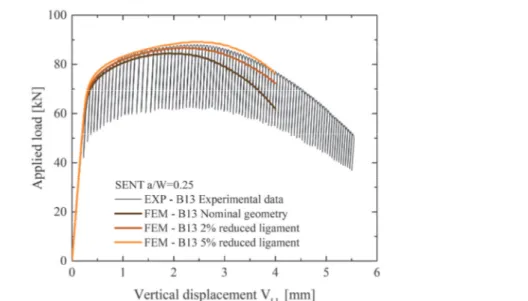
Crack propagation was simulated by means of element removal technique: when damage becomes critical at the element Gauss points, the element is removed and stresses are released. This feature, available in MSC MARC, does not suffer of convergence issues if the load step is relatively small to limit the overall number of elements that are removed at the same time. In Fig. 5 and Fig. 6, the comparison of the calculated response applied load vs displacement for SENT and SENB with experimental data is shown. For SENT a parametric investigation on the effect of the ligament size on the calculated applied load vs displacement response was performed. This analysis was motivated by the difference initially found using the nominal specimen dimensions in the simulation. It was found that an uncertainty of 5% (0.5 mm in this case) in the

(10)

323

ligament size has a significant effect on the predicted specimen response. A posteriori measurements confirmed such uncertainty in the effective crack ligament of machined samples.

a) d)

b) e)

c) f)

(11)

324

Figure 3: Failure locus for X65 BM showing the stress triaxiality vs plastic strain load path at the critical location in different notched bar samples.

Figure 4: Failure locus for X65 WM.

Figure 5: Comparison of calculated specimen response with experimental data for SENB sample. Multiple partial unloadings for R-curve determination are shown.

(12)

325 Figure 6: Comparison of calculated specimen response with experimental data for SENT sample. Results of FEM sensitivity analysis are given for different crack depths.

Figure 7: Comparison of calculated crack resistance curve for X65 BM with SENB a/W=0.25.

Finally, in Fig. 7 the comparison of predicted crack resistance with experimental data obtained using unloading compliance method, given in ASTM E-1820, is shown. In the simulation, the J-integral was calculated using the domain integral method [30]. Here, the comparison is very good all over the crack growth range of interest. At the intercept with the exclusion line, the error in the J-integral estimate is approximately 10%. At 0.2mm offset, the JIC is correctly predicted with an error of 1.7%.

C

ONCLUSIONS

n this work, the possibility to use CDM modelling to predict material strain capacity was demonstrated. The proposed modelling has the major advantage to capture correctly the effect of stress triaxiality on material ductility, which is critical for predicting the occurrence of rupture in ductile materials. This is of particular importance for high toughness materials, such as carbon steels operating in the right end side of ductile-to-brittle transition region, for which fracture mechanics validity limits are hard to be satisfied.

(13)

326

In its simplest implementation, the proposed damage model requires the identification of only two material parameters that can be determined performing simple tensile tests on round notched bar samples. The identification procedure, as discussed in this work, is suitable to be performed at industrial level and do not requires particular abilities.

The geometry transferability of material model parameters has been demonstrated predicting the crack growth in geometry samples with different crack tip constraints. In particular, it was shown that numerical simulation with CDM could be used to carry on “virtual experiments” for the determination of the material fracture toughness with high degree of accuracy. Consequently, the proposed CDM modelling could also be used to predict by simulation the resistance of components under different load/geometry configuration, reducing full-scale test effort for component qualification.

R

EFERENCES

[1] Mørk, K. The Challenges Facing Arctic Pipelines, Design Principles for Extreme Conditions. Offshore Oil and Gas Magazine, (2007) 67.

[2] Kan, W. C., Weir, M., Zhang, M. M., Lillig, D. B., Barbas, S. T., Macia, M. L., Biery, N. E. Strain-based pipelines: Design consideration overview. The Eighteenth International Offshore and Polar Engineering Conference,. International Society of Offshore and Polar Engineers (2008).

[3] Degeer, D., Nessim, M. Arctic pipeline design considerations. ASME 2008 27th International Conference on Offshore Mechanics and Arctic Engineering, American Society of Mechanical Engineers, (2008) 583-590.

[4] BS7910:2013 - Guide on Methods for Assessing the Acceptability of Flaws in Metallic Structures. BSI -British Standard Institute (2013).

[5] Schwalbe, K. H., Neale, B. K., Ingham, T., Draft EGF recommendations for determining the fracture resistance of ductile materials: EGF Procedure EGF P1–87D, Fatigue & Fracture of Engineering Materials & Structures, 11 (1988) 409-420.

[6] Gordon, J., Jones, R., Challenger, N., An experimental study to determine the limits of CTOD controlled crack growth. Constraint Effects in Fracture. ASTM International, (1993).

[7] Standard, A. Standard test method for measurement of fracture toughness. ASTM, E1820-01, (2016) 1-46.

[8] Moattari, M., Sattari-Far, I., Bonora, N. The effect of subcritical ductile crack growth on cleavage fracture probability in the transition regime using continuum damage mechanics simulation, Theoretical and Applied Fracture Mechanics, 82 (2016) 125-135.

[9] Det Norske Veritas Offshore Standard DNV‐OS‐F101. Submarine Pipeline Systems, (2012).

[10]Fehringer, F., Seidenfuß, M., Schuler, X., Experimental and numerical investigations on limit strains in ductile fracture. Procedia Structural Integrity, 2 (2016) 3345-3352.

[11]Acharyya, S., Dhar, S. A complete GTN model for prediction of ductile failure of pipe, Journal of Materials Science, 43 (2008) 1897.

[12]Xu, J., Zhang, Z., Østby, E., Nyhus, B., Sun, D., Constraint effect on the ductile crack growth resistance of circumferentially cracked pipes, Engineering Fracture Mechanics, 77 (2010) 671-684.

[13]Faleskog, J., Gao, X., Shih, C. F., Cell model for nonlinear fracture analysis–I. Micromechanics calibration. International Journal of Fracture, 89 (1998) 355-373.

[14]Bonora, N., COD of off-centred cracks in pipes under bending load: A geometrical solution. International Journal of Fracture, 75 (1996) 1-18.

[15]Bonora, N., Ruggiero, A., Esposito, L., Iannitti, G. Damage development in high purity copper under varying dynamic conditions and microstructural states using continuum damage mechanics, AIP Conference Proceedings, (2009) 107-110.

[16]Bonora, N., Ruggiero, A., Iannitti, G., Testa, G. Ductile damage evolution in high purity copper taylor impact test. AIP Conference Proceedings, (2012) 1053-1056.

[17]Chiantoni, G., Bonora, N., Ruggiero, A., Experimental study of the effect of triaxiality ratio on the formability limit diagram and ductile damage evolution in steel and high purity copper. International Journal of Material Forming, 3 (2010) 171-174.

[18]Carlucci, A., Bonora, N., Ruggiero, A., Iannitti, G., Gentile, D., Crack initiation and growth in bimetallic girth welds. Proceedings of the International Conference on Offshore Mechanics and Arctic Engineering - OMAE, (2014).

[19]Bonora, N., Carlucci, A., Ruggiero, A., Iannitti, G., Simplified approach for fracture integrity assessment of bimetallic girth weld joint. Proceedings of the International Conference on Offshore Mechanics and Arctic Engineering - OMAE, (2013).

(14)

327

[20]Kachanov, L. M., On Creep Rupture Time. Izv. Acad.Nauk. SSSR, Otd.Techn. Nauk, (1958) 8. [21]Lemaitre, J., Micro-mechanics of crack initiation. International journal of fracture, (1990) 42, pp. 87-99.

[22]Pirondi, A., Bonora, N., Modeling ductile damage under fully reversed cycling. Computational Materials Science, 26 (2003) 129-141.

[23]Bonora, N., A nonlinear CDM model for ductile failure. Engineering Fracture Mechanics, 58 (1997) 11–28.

[24]Iannitti, G., Bonora, N., Bourne, N., Ruggiero, A., Testa, G., Damage development in rod-on-rod impact test on 1100 pure aluminum. AIP Conference Proceedings, (2017).

[25]Iannitti, G., Bonora, N., Ruggiero, A., Testa, G., Ductile damage in Taylor-anvil and rod-on-rod impact experiment. Journal of Physics: Conference Series, (2014) 500.

[26]Bonora, N., Ruggiero, A., Gentile, D., De Meo, S., Practical applicability and limitations of the elastic modulus degradation technique for damage measurements in ductile metals. Strain, 47 (2011) 241-254.

[27]Gambirasio, L., Chiantoni, G., Rizzi, E., On the Consequences of the Adoption of the Zaremba–Jaumann Objective Stress Rate in FEM Codes. Archives of Computational Methods in Engineering, 23 (2016) 39-67.

[28]Oh, C.-K., Kim, Y.-J., Baek, J.-H., Kim, Y.-P., Kim, W.-S., Ductile failure analysis of API X65 pipes with notch-type defects using a local fracture criterion. International Journal of Pressure Vessels and Piping, 84 (2007) 512-525. [29]Bonora, N., Ruggiero, A., Esposito, L., Gentile, D., CDM modeling of ductile failure in ferritic steels: Assessment of

the geometry transferability of model parameters, International Journal of Plasticity, 22 (2006) 2015-2047.

[30]Shih, C., Moran, B., Nakamura, T., Energy release rate along a three-dimensional crack front in a thermally stressed body. International Journal of fracture, 30 (1986) 79-102.