HAL Id: hal-00905791
https://hal.archives-ouvertes.fr/hal-00905791
Submitted on 20 Feb 2014
HAL is a multi-disciplinary open access
archive for the deposit and dissemination of
sci-entific research documents, whether they are
pub-lished or not. The documents may come from
teaching and research institutions in France or
abroad, or from public or private research centers.
L’archive ouverte pluridisciplinaire HAL, est
destinée au dépôt et à la diffusion de documents
scientifiques de niveau recherche, publiés ou non,
émanant des établissements d’enseignement et de
recherche français ou étrangers, des laboratoires
publics ou privés.
Polarization Twisting Element
Shoaib Muhammad, Ronan Sauleau, Guido Valerio, Laurent Le Coq, Hervé
Legay
To cite this version:
Shoaib Muhammad, Ronan Sauleau, Guido Valerio, Laurent Le Coq, Hervé Legay. Self-Polarizing
Fabry-Perot Antennas Based on Polarization Twisting Element.
IEEE Transactions on
Anten-nas and Propagation, Institute of Electrical and Electronics Engineers, 2013, 61 (3), pp.1032-1040.
�10.1109/TAP.2012.2227443�. �hal-00905791�
Abstract— A new configuration of self-polarizing Fabry-Perot
(FP) antenna is presented to generate circular polarization with high gain levels using a simple linearly-polarized feed. It consists of a FP resonator combined with a polarization-twisting ground plane. An analytical model is proposed to facilitate the antenna design, and the corresponding results are shown to be in very close agreement with full-wave simulations. The experimental prototype built in C-band exhibits a combined bandwidth (3 dB axial ratio, 3dB gain drop, and -10 dB impedance matching) of 3% with a maximum realized gain of 18.0 dB. The antenna is completely shielded with an aperture size of 4.0λ0 4.0λ0 and a
height of only λ0. Such antennas are attractive candidates for
high-power space applications at low frequencies (L- to C-bands) where standard horns are very bulky.
Index Terms— Circular polarization, self-polarization,
Fabry-Perot resonators, horns.
I. INTRODUCTION
HE original concept of Fabry-Perot (FP) antennas [1] has received a lot of attention over the last years. The main reason is that these antennas allow achieving high gain while keeping low profile structures [2]-[4]. Most of the previous studies focused on linearly-polarized (LP) FP antennas (e.g. [5]-[8]).
Recently, new configurations called self-polarizing FP cavity antennas have been proposed [9], [10]. The aim is to avoid using circular polarization (CP) feed networks that are usually bulky for high power applications from L- to C-bands [11], and to replace them by simple LP feeds exciting the FP antenna element. The particularity of this concept is that the antenna itself generates the CP and provides high gain simultaneously.
In [9], a three-layered Frequency Selective Surface (FSS) structure is placed over a metallic ground plane to combine the FP and self-polarizing effects. The experimental results obtained for a 9λ0 9λ0 1.8λ0 antenna size have shown good
results: combined bandwidth (3-dB axial ratio (AR) and -10 dB impedance matching) of 2.24%, and maximum measured gain of about 21 dB.
The configuration introduced in [10] is very different. The
Manuscript received February 7th, 2012. This work has been carried out at
the “Institut d'Electronique et de Télécommunications de Rennes”, IETR, Rennes, France. The project was financed by Thales Alenia Space, France.
S. A. Muhammad, R. Sauleau, G. Valerio, and L. Le Coq are with IETR, UMR CNRS 6164, University of Rennes 1, Rennes, France. Email:
[email protected], ronan.sauleau, guido.valerio,
H. Legay is with Thales Alenia Space, France, 31037 Toulouse Cedex 1, France (email: [email protected]).
authors proposed to combine a single-layered polarizing FSS and linear corrugations to control at the same time the polarizing and FP effects. The corresponding antenna is very compact (1.6λ0 1.6λ0 0.8λ0) but exhibits a much narrower
combined bandwidth (around 1.4%) with a 13.3 dB maximum gain.
A new self-polarizing antenna configuration is studied here. The idea consists in using a non-resonant FSS to produce the FP resonance and a polarizing twisting surface to generate the CP with an improved bandwidth in terms of AR and impedance matching.
The outline of this paper is as follows. In Section II.A, the antenna concept is presented, along with its geometry and working principle. As there are many parameters to be optimized, an analytical model is proposed to facilitate the pre-design of the antenna (Sections II.B and II.C). Full-wave simulation results and experimental data are compared in Section III. The conclusions are drawn in Section IV.
II. ANTENNA CONCEPT AND MODELING
A. Basic idea and antenna geometry
The main idea is to separate the FP resonance effect and the CP generation part. To this end, we can imagine a simple FP resonator (Fig. 1) composed of two partially reflecting surfaces or FSS (with their respective reflection and transmission coefficients); both FSS are separated by a distance Dcav
dictated by the classical resonance condition at f0,
([1],[5],[12]) 2 2 2 2 1 0 N f c D x x cav , (1)
where c is the speed of light in vacuum, and N is an integer (N = 0, 1, 2, …). ρ1x and ρ2x are the reflection coefficient phase
values of the lower and upper FSS respectively.
When this resonator is excited by a source element (waveguide, patch, etc.) placed between the two FSS, the antenna resonates at f0 and, depending on the FSS
characteristics [1],[2],[12], a highly-directive wave is radiated on both sides of the resonator (i.e. in +z and –z directions). If both FSS have the same reflectivity, the magnitude of energy is the same in both directions.
Let us consider now that the resonator is excited in linear polarization (e.g x-polarization) and is made with two one-dimensional (1-D) FSS that are highly-reflective for only one polarization (x-polarization here) and nearly-transparent for the orthogonal one (y-polarization), as shown in Fig. 1; this
Self-polarizing Fabry-Perot Antennas Based on
Polarization Twisting Element
Shoaib Anwar Muhammad, Ronan Sauleau, Senior Member, IEEE, Guido Valerio, Member, IEEE,
Laurent Le Coq, and Hervé Legay
twisting element is placed on one side of the FP resonator (like corrugations tilted at 45° as illustrated in Fig. 1), it will convert the incident x-polarized wave Ex into a reflected
y-polarized wave Ey which travels back to the FP resonator. As
the latter is transparent to y-polarization (Appendix B), the energy passes through the cavity without any disturbance. By controlling the distance between the resonator and the polarization twister (Dp), a 90°-phase difference between the
two orthogonal polarizations can be obtained. Consequently, both components Ex and Ey combine each other in the upper
space to produce a CP wave. A similar concept has been reported in literature for the design of folded reflectarrays using a planar polarization twister, e.g. [13],[14].
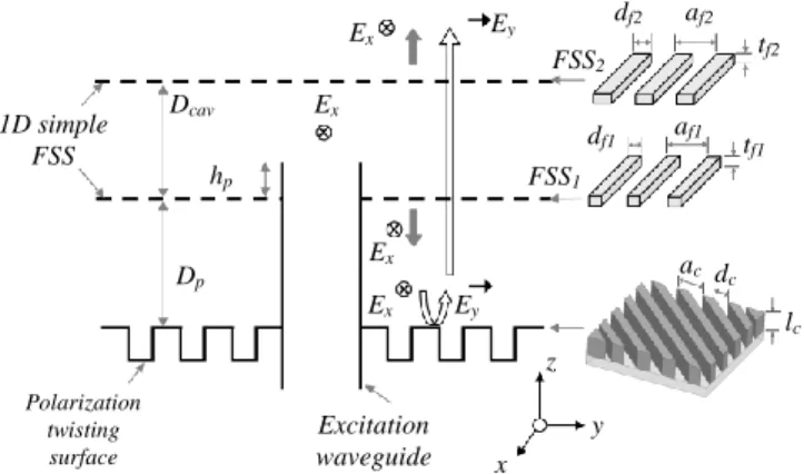
Fig. 1. Proposed antenna configuration. Both FSS are 1-D inductive grids along x-direction. The twisting surface is made of horizontal corrugations tilted at 45°.
B. Analytical model
The antenna architecture is defined by many parameters (FSS and twister dimensions, Dcav, Dp, hp, etc.). An analytical
model is presented here to facilitate its pre-design. This model is based on the multiple-reflection approach (e.g. [1],[12]) where an infinite FP interferometer is modeled using ray tracing. This model provides good results for antenna apertures in the order of few wavelengths or larger, e.g. [6].
The analytical model implemented here is summarized in Fig. 2. It consists of an infinite FP resonator with two 1-D FSS elements (as those shown in Fig. 1) characterized by their respective reflection (r1x, r2x) and transmission coefficients (t1x,
t2x) and separated by a distance Dcav. The polarization twister
(metallic corrugations at 45°, Fig. 1) is modeled by its reflection coefficient rcy representing the polarization
conversion of an incident x-polarized wave into a reflected y-polarized wave. The excitation element is assumed to be a waveguide source radiating in the +z direction, placed at a distance hp from the bottom FSS. Using the ray-tracing
method, and assuming that the point source is linearly-polarized with unit magnitude (i.e. |Einc| = 1) and that there is
no loss in the antenna and twister parts, the paths traced by the rays emitted by the source are represented in Fig. 2.
To calculate the axial ratio of this antenna, we first need to find the transmission coefficients x
FP
T and T in x- and y-FPy
polarizations. Each transmission coefficient is simply the
after an infinite number of multiple reflections between the two FSS.
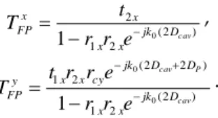
Using the simple procedure outlined in Appendix A along with an infinite series summation formula, the transfer function for both polarizations can be expressed as follows
) 2 ( 2 1 2 0 1 jk Dcav x x x x FP e r r t T , (2) ) 2 ( 2 1 ) 2 2 ( 2 1 0 0 1 cav P cav D jk x x D D jk cy x x y FP e r r e r r t T . (3)
It is important to mention here that, only the broadside values (θ = 0°) of the transfer functions are retained as the antenna directivity is maximum at broadside. For configurations where the maximum directivity is required for other angles, the cosθ term can be included in the model for optimization (Appendix A).
Next, the axial ratio can be easily computed from Equ. (2) and (3) using the following expression
) ( sin 4 ) ( sin 4 2 2 2 2 G G G G AR (4) where G = ρL + 1/ρL, ρL = TFPx TFPy , and φ = TFPx –TFPy.
Fig. 2. Analytical model of the proposed antenna based on ray-tracing method. The rays for x-polarization are represented as black dots, and the rays presenting the y-polarized ray by grey dots.
C. Analytical optimization
The analytical model presented above is implemented here to optimize the antenna parameters. The following procedure is employed.
For a given FSS configuration (r1x, r2x, t1x, t2x) and twister
characteristics (rcy), the antenna height parameters (Dcav, Dp)
are varied in order to obtain the broadest 1-dB AR bandwidth with the maximum of the transfer function centered around f0.
The FSS characteristics (r1x, r2x, t1x, t2x) can be obtained either
analytically for 1-D inductive grids with zero thickness (e.g. [15]-[17]) or numerically using full-wave simulations and periodic boundary conditions for more complex FSS shapes. The later method has been chosen here because rigid and thick metallic FSS screens without any dielectric support are required here for high-power space applications.
hp
Dcav
Dp
Source
Corrugations @ 45° in the XoY plane z x y (r2x, t2x) (r1x, t1x) (rcy) θ Excitation waveguide hp Dcav Dp df2 1D simple FSS af2 tf2 df1 af1 tf1 ac dc lc Polarization twisting surface x y z Ex Ex Ey Ey Ex Ex FSS1 FSS2
The parameter rcy is calculated in the same way, using
periodic boundary simulations (HFSS) around a unit-cell of linear corrugation (tilted by 45°), and by illuminating it with a plane wave polarized along x and observing the reflection coefficient in y-direction. The reference curves for the most interesting cases are detailed in Appendix B.
It should also be noted here that this model can be used also for planar self-polarizing antennas by including a dielectric substrate with a FSS etched on both sides and a planar twister element (as the one reported in [18]).
(a)
(b)
(c)
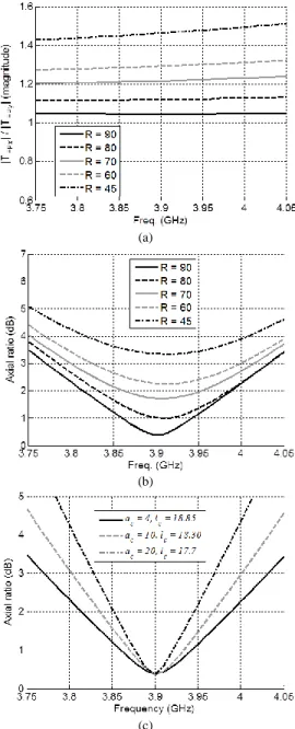
Fig. 3. Analytical results. Impact of the FSS reflectivity R (for a fixed twister configuration, ac = 4 mm, lc = 18.85 mm) on (a) the ratio of the transfer functions |TFPx| / |TFPy|, and (b) the axial ratio. (c) Impact of the twister configuration (ac and lc, in mm) on the axial ratio bandwidth (with a fixed
FSS reflectivity R = 90%).
To keep a simple antenna structure, thick 1-D inductive grids and rectangular corrugations are used. Their typical frequency responses are given in Appendix B. This data base is employed to pre-define the antenna geometry and select the best set of parameters providing the largest AR bandwidth and
the highest directivity at broadside (θ = 0°) which is indicated by the magnitude of the transfer function calculated from (2) and (3). For optimization runs, the values of Dcav and Dp are
varied over a wide range of values around a central starting value. The starting point for Dcav is calculated using equation
(1), while the starting point for Dp is chosen to be around a
quarter wavelength (λ0/4). Then a range of values around these
starting values is selected (first a wide range with large steps, then a finer range with smaller steps for fine tuning) to calculate the transfer functions and the axial ratio over a given frequency band and a given FSS reflectivity pair for the two FSS layers.
For this study, both FSS are identical in order to radiate the same energy in both directions, and the losses are assumed to be negligible. Some representative results are represented in Fig. 3.
In Fig. 3(a), the antenna transfer function ratios (from Equ. (2) and (3)) are shown for different FSS reflectivity values (R = R1 = R2), where R1 = |r1x|² and R2 =|r2x|². It can be observed
that as R is decreased, the magnitude of the x-polarized wave becomes more important than the y-polarized one. In other words, the ratio |TFPx| / |TFPy| between the two transfer functions
is increased. This is an expected result due to waveguide type of excitation source used to model this antenna. As the FSS reflectivity is decreased, there is less energy going towards the twister. Hence, the antenna does not produce good quality circularly polarized wave for lower FSS reflectivity values. Consequently, the AR curves (Fig. 3(b)) degrade for lower values of R. Using a source which radiates equally towards both +z and -z directions (for example a dipole) would remedy this problem; but in this study, the waveguide source is retained as requested by Thales Alenia Space, France.
Fig. 3(c) shows that, for a fixed value of R, the use of a smaller twister periodicity ac leads to an enlargement of the
AR bandwidth. The value of lc is adjusted to ensure that the
twister operates around the center frequency of 3.9 GHz. The transfer function ratio for a fixed reflectivity and a variable twister periodicity (not shown here) does not change.
From the above results, we can infer that we must use highly reflective FSS in order to ensure a good quality circularly polarized wave. On the other hand, the twister configuration has a direct impact on the AR bandwidth, but does not modify the antenna radiation characteristics.
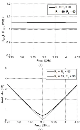
To further improve the proposed configuration, we studied the analytical model with different FSS reflectivity values to compensate for the difference between the x- and y-polarized transfer function magnitudes. The case with R = 90%, ac = 4
mm, and lc = 18.85 mm, was selected as it provides the best
axial ratio bandwidth. The reflectivity of the lower FSS (FSS1
in Fig. 1) was lowered to allow for more energy to go towards the twister. The best results (observed for R1 = |r1x|² = 89% and
R2 =|r2x|² = 90%) are shown in Fig. 4 and compared to the case
with equal FSS reflectivity values. We observe that we obtain equal magnitude for both transfer functions (Fig. 4(a)) and better axial ratio minima (Fig. 4(b)) as compared to the case where both FSS have same reflectivity values. However, the
The best case selected from this optimization study is the one with R1 = 89% (af1 = 25 mm, df1 = 4.5 mm), and R2 =90%
(af2 = 25 mm, df2 = 5 mm) and a twister configuration with ac =
4 mm, lc = 18.85 mm (largest AR bandwidth). In this case, a
3-dB AR bandwidth of about 6.7% is obtained for Dcav = 32.2
mm and Dp = 7.7 mm. The other dimensions (FSS and twister)
can be found in Appendix B.
(a)
(b)
Fig. 4. Comparison between the analytical results using same (R1 = R2 = 90%) and different (R1 = 89%, and R2 = 90%) FSS reflectivity values for the upper and lower FSS (for a fixed twister configuration, ac = 4 mm, lc = 18.85 mm) (a) the magnitude of the transfer functions |TFPx| and |TFPy|, (b) and the axial ratio.
III. SIMULATION AND EXPERIMENTAL RESULTS
A. Full-wave optimization
Once the concept has validated analytically, the next step is to simulate a finite antenna using a full-wave simulation tool. For this, HFSS has been used to simulate an antenna with a square aperture and shielding cavity walls for better integration into an array configuration and to minimize coupling between neighboring sources [8], [10]. The simulation setup and the dimensions are defined in Fig. 5. The antenna aperture size (defined by Thales Alenia Space, France) is about 4λ0 so as to produce a pencil beam with a
directivity of about 20 dBic in C-band (f0 = 3.9 GHz).
The antenna is fed by a standard rectangular waveguide (WR229) with interior dimensions of 58.17 29.08 mm² (twg = 5mm). This waveguide penetrates through the twister
part into the FP cavity (as schematized in Fig. 1). The impedance matching is optimized by varying the waveguide penetration inside the cavity (hp) and the iris width (di) placed
have confirmed the relevance of this impedance matching system [8], [10].
A parametric study has been carried out with HFSS in order to take into account the finite size effects and the presence of shielding walls which were not modeled in Section II.B. This study consists in three steps: i) the FSS parameters and cavity height (Dcav) are varied to obtain the maximum directivity, ii)
the corrugation parameters and the distance (Dp) is then
adjusted to obtain the maximum 1-dB AR bandwidth, iii) finally, the impedance matching level is improved by adjusting the waveguide penetration hp and iris width di.
TABLE I
FINAL DIMENSIONS FOR THE SELF-POLARIZING FP ANTENNA (AS A REMINDER,
THE DIMENSIONS OPTIMIZED ANALYTICALLY ARE GIVEN INTO BRACKETS)
Antenna aperture (Lant) 320 mm
Antenna height (hant) 73.0 mm
Cavity height Dcav = 32.5 mm (32.2 mm)
Dp = 6.5 mm (7.7 mm) Corrugation parameters lc = 16.0 mm (18.85 mm) dc = 3.0 mm (3.0 mm) ac = 4.0 mm (4.0 mm) FSS parameters af1 = af2 = 25 mm (25.0 mm) tf1 = tf2 = 5 mm (5.0 mm) df1 = 4.0 mm (4.5 mm) df2 = 6.5 mm (5.0 mm)
Impedance matching part di = 8.0 mm, hp = 10 mm, ti = tp = 1 mm
(a)
(b)
Fig. 5. Simulation setup. (a) 3D cross-section view (half antenna). (b) Cross-section view.
The final dimensions are given in Table I. We can observe that they are rather close to those derived from the analytical optimization (Section II.C). The width of the top FSS (df2) is
larger than the bottom one (df1) as predicted by the analytical
model. This allows for more energy flowing towards the twister as compared to the energy leaving the FP cavity
Dcav Dp lc tw tw tf2 tf1 hp ac dc df2 af2 af1 df1 tp ti di awg Lant hant twg Cavity Corrugations @ 45° Rectangular waveguide Waveguide penetration Iris FSS2 FSS1
towards the +z direction. In other words, the reflectivity value of the bottom FSS layer is slightly lower as suggested by the analytical model. In the optimized design, the reflectivity of FSS1 and FSS2 at 3.9 GHz equal 88% and 95% respectively.
This difference with the analytical results is due to the combined effect of the finite size of the antenna, the close proximity of shielding walls, and the size of the waveguide source which were not taken into account in the analytical model.
The cavity wall thickness tw equals 8mm. The total antenna
height hant is only 73 mm (0.95λ0) without the excitation
waveguide source.
(a)
(b)
(c)
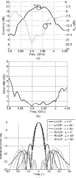
Fig. 6. Simulation results. (a) Directivity, Reflection coefficient.
(b) Axial ratio, (c) Radiation patterns in LHCP and RHCP @ 3.90 GHz.
B. Optimization results
The simulation results of the optimized configuration are summarized in Fig. 6. A maximum directivity of about 20 dBic is achieved at 3.93 GHz with a reflection coefficient below -17.5 dB (Fig. 6a). The 3-dB AR bandwidth equals 5.1% (3.82 GHz – 4.02 GHz, Fig. 6b). This value is slightly lower than the one predicted analytically (6.7%). The main reason for this
difference is the presence of the surrounding cavity walls, the finite size of the antenna, and the presence of the waveguide. The left- and right-hand CP radiation patterns are shown in Fig. 6c at 3.90 GHz (frequency point where the AR is minimum). Very clean patterns with side lobe level lower than -13.5 dB and cross-polarization level below -17.5 dB are obtained for all observation planes.
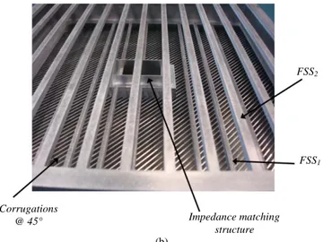
C. Prototyping and experimental results
The optimized antenna (dimensions given in Table I) has been manufactured in separated parts. The FSS have been fabricated using water-jet cutting technology, the twister surface with a CNC milling machine, while the waveguide, the impedance matching system, and the cavity walls were produced using a manual milling machine. The assembled antenna is shown in Fig. 7 with its supporting structure for measurement purposes.
The measurement results are shown in Fig. 8. A maximum directivity level of about 18.5 dBic is measured at 3.9 GHz, with a reflection coefficient S11 below -18 dB (Fig. 8a). A
maximum realized gain of 18 dB is measured. The 0.5 dB difference between the measured directivity and realized gain is very likely due to the cumulative effects of fabrication, assembly and alignment errors. The measured S11 is lower than
-18 dB over the entire 3-dB gain drop bandwidth. The measured 3dB axial ratio bandwidth is about 4.6% (3.81 GHz – 3.99 GHz, Fig. 8b). Again, the frequency shift (~ 25 MHz, i.e. 0.6 %), observed between measurements and simulations, is attributed to fabrication uncertainties.
(a) Corrugations @ 45° 320 mm (4λ0) 73 mm (0.95λ0) Supporting structure FSS2 FSS1
(b)
Fig. 7. Fabricated prototype for operation in C-band. (a) 3D view with the supporting structure. (b) Zoomed view.
As a summary, a combined bandwidth of 3% (3 dB axial ratio bandwidth, 3dB gain drop bandwidth and -10 dB impedance matching) has been obtained experimentally (3.84 GHz – 3.96 GHz). This value is significantly better than the self-polarizing solutions proposed in [9] (much compact) and [10] (more efficient). Finally the measured CP patterns at 3.90 GHz (Fig. 8c) show similar behavior as in simulations. The 3dB gain drop bandwidth could be improved further by using tapered reflectivity for the FSS [19].
(a)
(b)
(c)
(d)
Fig. 8. Comparison between simulation and measured results. (a) Directivity, and realized gain, (b) axial ratio, (c) reflection coefficient, (d) measured radiation patterns in LHCP and RHCP @ 3.90 GHz.
The axial ratio variation with respect to θ at 3.9 GHz is shown in Fig. 9 in simulations and measurement. Both results are in excellent agreement. From simulations, we have a 3dB axial ratio beamwidth of about 24° around the axial direction, while the measurements show a beamwidth of 20°.
(a)
(b)
Fig. 9. Angular variation of axial ratio @ 3.90 GHz. (a) Simulation, and (b) measurements. Corrugations @ 45° Impedance matching structure FSS2 FSS1
IV. CONCLUSION
A new concept of self-polarizing FP antennas simultaneously combining the principles of FP resonators and polarizing twisting elements has been studied analytically, numerically and experimentally. The antenna pre-design is defined using an analytical model based on ray-tracing. Then, full-wave optimization results for a finite antenna have been presented and successfully validated around 3.9 GHz. This concept is quite general and could be extended to planar antennas for low-power applications.
APPENDIX
A. Analytical calculations
Using the definitions of Fig. 2, the transfer function for the x- and y-polarized waves can be written as a sum of all fields transmitted in the far-field region (assuming the source position (hp) as the reference plane)
...] [ ) ( '' 1 ' 1 x tx x inc trans x FP E E E E x E T (A-1) ...] [ ) ( ' '' ty ty ty inc trans y FP E E E E y E T (A-2)
where Einc = 1, Etx, E’tx, E’’tx, etc. are the far-field rays
generated by multiple reflections of the incident wave between the two FSS layers; and Ety, E’ty, E’’ty, etc. are the far field rays
generated by the corrugations at 45° (twister surface). It is assumed here that there is no x-component reflected from the corrugations (i.e |rcx| = 0) and the FSS layers are completely
transparent to the y polarized wave coming from the corrugations (i.e |r1y| = |r2y| = 0, and |t1y| = |t2y| = 1). These
assumptions hold true over the small frequency band around the central design frequency (see section B) and consequently simplify a great deal the analytical model.
Now, by replacing these rays by the corresponding reflection and transmission coefficients of the FSS and the twister, we obtain ([1], [5], [12]) ...] [ 2 (4 )cos 2 2 1 2 cos ) 2 ( 2 1 2 2 0 0 cav jk Dcav x x x D jk x x x x x FP t t r r e t r r e T (A-3) 2 (2 4 )cos 2 1 1 cos ) 2 2 ( 2 1 0 0 [ P cav jk DP Dcav x x cy x D D jk x cy x y FP t rr e t r rr e T 1 1223 jk0(2DP6Dcav)cos...] x x cy xr r r e t (A-4) where θ is the incidence angle of the excitation wave, and k0
is the wave number in free space.
The above equations can be transformed easily using infinite series summation; which gives
cos ) 2 ( 2 1 2 0 1 jk Dcav x x x x FP e r r t T , (A-5) cos ) 2 ( 2 1 cos ) 2 2 ( 2 1 0 0 1 cav P cav D jk x x D D jk cy x x y FP e r r e r r t T . (A-6)
In our calculations, we assume θ = 0° as we are interested only in the antenna characteristics at broadside. Finally, we have: ) 2 ( 2 1 2 0 1 jk Dcav x x x x FP e r r t T , (A-7) ) 2 ( 2 1 ) 2 2 ( 2 1 0 0 1 cav P cav D jk x x D D jk cy x x y FP e r r e r r t T . (A-8)
B. Reference curves used for analytical study
Inductive FSS: The analytical results of Section II.B have been generated using a set of reference curves for the FSS reflection (r1x, r2x) and transmission (t1x, t2x) coefficients, and
for the corrugated twister (rcy). These curves have been
computed with HFSS (as explained in Section II.C) as a function of frequency around the central frequency (3.9 GHz here).
The FSS periodicity considered in this paper (Fig. 1) is given in Table II. The FSS thickness (tf1 = tf2) and width (df1 =
df2) are constant for all cases (5 mm).
TABLE II
FSS DIMENSIONS FOR DIFFERENT REFLECTIVITY VALUES
Reflectivity (%) R = 2 2 2 1x rx r 90 80 70 60 45 Periodicity (mm) af1 = af2 25 30 33.5 36 40 (a) (b) (c) (d)
Fig. 10. HFSS simulation results for FSS with reflectivity values ranging between 45% and 90%. Reflection coefficient in magnitude (a) and phase (b). Transmission coefficient in magnitude (c) and phase (d). Both FSS are assumed identical.
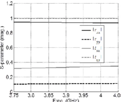
To validate the assumption made in the previous section (section A) and stating that the FSS is completely transparent to the y-polarized wave coming from the corrugations below, the S-parameters for the 90% reflectivity case are shown in Fig. 11 for x- and y-polarized plane wave excitation. It can be seen that the transmission coefficient is nearly equal to 1 and a very low level of y-polarized energy is reflected by the FSS. Hence, the assumptions in the previous calculations (|r1y| = |r2y|
Fig. 11. S-parameters for the x- and y-polarized incident plane waves on a 1D FSS infinite surface (HFSS simulations) with 90% reflectivity.
Corrugated twister: We assume that the width dc of the
corrugations equals 3 mm in all cases. Only their periodicity ac
and depth lc are varied to make the twister operating around f0
= 3.9 GHz.
Three relevant and representative twister configurations are selected here (Fig. 12). Their reflection coefficients in y-direction (for a normally incident plane wave polarized along x-direction) are plotted in amplitude and phase for three values of ac and lc in Fig. 12(a) and (b). We can see from Fig. 12(a)
that, for ac = 4 mm and lc = 18.85 mm, we obtain the largest
bandwidth over which the energy is converted from x- to y-polarization, while form Fig. 12(b) we can see that the phase is nearly constant around 180° for the same case (ac = 4 mm, lc =
18.85 mm). This explains why we obtain the widest AR bandwidth using this twister configuration.
(a) (b)
Fig. 12. HFSS simulation results for an infinite flat corrugated surface tilted at 45° and illuminated by a x-polarized plane wave under normal incidence. Reflection coefficient rcy in magnitude (a) and phase (b) for three values of ac and lc.
Fig. 13. Reflection coefficient in the x-polarized and y-polarized wave from the corrugations with an incident x-polarized plane wave for ac = 4 mm, lc = 18.85 mm and dc = 3 mm.
The magnitude of the x- and y-polarized components reflected from the corrugations is shown in Fig. 13. We can see that the x-polarized field is negligible and hence the assumptions for the calculations in the previous sections are valid (i.e |rcx| = 0).
This work was performed using HPC resources from GENCI-IDRIS (grant 2012-050779).
REFERENCES
[1] G. V. Trentini, “Partially reflecting sheet arrays,” IRE Trans. Antennas
Propag., vol. 4, no. 4, pp. 666–671, Oct. 1956.
[2] D. R. Jackson and A. A. Oliner, “A leaky-wave analysis of the high-gain printed antenna configuration,” IEEE Trans. Antennas Propag., vol. 36, no. 7, pp. 905–910, Jul. 1988.
[3] R. Sauleau, Ph. Coquet, J.-P. Daniel, T. Matsui, and N. Hirose, “Study of Fabry-Perot cavities with metal mesh mirrors using equivalent circuit models. Comparison with experimental results in the 60 GHz band,” Int.
Journ. Infrared Millimeter Waves, vol. 19, no. 12, pp. 1693–1710, Dec.
1998.
[4] M. Thèvenot, C. Cheype, A. Reineix, and B. Jecko “Directive photonic band-gap antennas,” IEEE Trans. Microwave Theory Tech., vol. 47, no. 11, pp. 2115–2122, Nov. 1999.
[5] A. P. Feresidis, G. Goussetis, S. Wang, and J. C. Vadaxoglou, “Artificial magnetic conductor surfaces and their application to low profile high-gain planar antennas,” IEEE Trans. Antennas Propag., vol. 53, no. 1, pp. 209–215, Jan. 2005.
[6] O. Roncière, B. A. Arcos, R. Sauleau, K. Mahdjoubi, and H. Legay, “Radiation performance of purely metallic waveguide fed compact Fabry Perot antennas for space applications,” Microw. Opt. Technol.
Lett., vol. 49, no. 9, pp. 2216–2221, Sep. 2007.
[7] N. Llombart, A. Neto, G. Gerini, M. Bonnedal, and P. de Maagt, “Leaky wave enhanced feed arrays for the improvement of the edge of coverage gain in multibeam reflector antennas,” IEEE Trans. Antennas Propag., vol. 56 , no. 4, pp. 1280–1291, May 2008.
[8] S. A. Muhammad, R. Sauleau, and H. Legay, “Small size shielded metallic stacked Fabry-Perot cavity antennas with large bandwidth for space applications,” IEEE Trans. Antennas Propag., vol. 60, no. 2, pp. 792–802, Feb. 2012.
[9] E. Arnaud, R. Chantalat, Th. Monédière, E. Rodes, and M. Thèvenot, “Performance enhancement of self-polarizing metallic EBG antennas,”
IEEE Antenna Wireless Propag. Lett., vol. 9, pp. 538–541, May 2010.
[10] S. A. Muhammad, R. Sauleau, and H. Legay, “Self generation of circular polarization using compact Fabry-Perot antennas,” IEEE
Antenna Wireless Propag. Lett., vol. 10, pp. 907–910, Sep. 2011.
[11] S. M. H. Chen and G. N. Tsandoulas, “A wide-band square-waveguide array polarizer,” IEEE Trans. Antennas Propag., vol. 21, no. 3, pp. 389–391, May 1973.
[12] R. Sauleau, “Fabry Perot resonators,” Encyclopedia of RF and Microwave Engineering, Ed. Chang, K., John Wiley & Sons, Inc., vol. 2, pp.1381–1401, ISBN: 0-471-27053-9, May 2005.
[13] P. W. Hanan, “Microwave antennas derived from the Cassegrain telescope,” IRE Trans. Antennas Propag., vol. AP-9, pp. 140-153, Mar. 1961.
[14] V.G. Borkar, V.M. Pandharipande, and R. Ethiraj, “Millimeter wave twist reflector design aspects,” IEEE Trans. Antennas Propagat., vol. 40, no. 11, pp. 1423–1426, Nov. 1992.
[15] O. Luukkonen, C. Simovski, G. Granet, G. Goussetis, D. Lioubtchenko, A. V. Raisanen, and S. A Tretyakov, “Simple and accurate analytical model of planar grids and high-impedance surfaces comprising metal strips or patches,” IEEE Trans. Antennas Propagat., vol. 56, no. 6, pp. 1624–1632, Jun. 2008.
[16] R. Sauleau, Ph. Coquet, and J.-P. Daniel, “Validity and accuracy of equivalent circuit models of passive inductive meshes. Definition of a novel model for 2D grids,” Int. Journ. Infrared Millimeter Waves, vol. 23, no. 3, pp. 475–498, Mar. 2002.
[17] B. A. Munk, Frequency Selective Surfaces: Theory and Design, J. Wiley & Sons. Inc., 2000.
[18] E. Doumanis, G. Goussetis, J.-L. Gomez-Tornero, R. Cahill, and V. Fusco, “Anisotropic impedance surfaces for linear to circular polarization,” IEEE Trans. Antennas Propag., vol. 60, no. 1, pp. 212– 219, Jan. 2012.
[19] X. He, W.X. Zhang, and D.L. Fu, “A broadband compound printed air-fed array antenna,” International conf. Electromagnetics in advanced