Exploring optimal snoRNA profiling using Next Generation Sequencing methods

Exploration des méthodes de séquençage pour une identification optimale des snoRNAs

Par

Fabien Dupuis-Sandoval Programmes de Biochimie

Mémoire présenté à la Faculté de médecine et des sciences de la santé en vue de l’obtention du grade de maitre ès sciences (M. Sc.)

en Biochimie

Sherbrooke, Québec, Canada Octobre, 2017

Membres du jury d’évaluation Michelle Scott, Biochimie Martin Bisaillon, Biochimie

Pierre-Étienne Jacques, Biologie, Université de Sherbrooke

S

Résumé

Exploration des méthodes de séquençage pour une identification optimale des snoRNAs

Par

Fabien Dupuis Sandoval Programmes de Biochimie

Mémoire présenté à la Faculté de médecine et des sciences de la santé en vue de l’obtention du diplôme de maitre ès sciences (M.Sc.) en Biochimie, Faculté de médecine et des sciences de la santé, Université de Sherbrooke, Sherbrooke, Québec, Canada, J1H 5N4 Des avancées récentes dans le domaine du séquençage de prochaine génération ont ouvert une panoplie de façons de générer des données. Toutefois, chaque nouvelle méthode dévelopée est souvent appropriée à la caractérisation d’un seul type de phénomène ou de molécules. L’objectif de cette analyse est d’identifier la manière la plus appropriée de générer et traiter les données pour étudier les petits ARNs nucléolaires, snoRNAs. Récemment, ceux-ci ont été révélés comme des acteurs dans une variété de fonctions alternatives comme l’épissage alternatif, la résistance au choc oxidatif et l’état de la chromatine. Il est donc impératif de trouver une méthode qui puisse traiter une large quantité de données contenant les snoRNAs et leurs intéracteurs pour découvrir les rôles encore inexplorés des snoRNAs. Dans cette optique, un nouveau protocole a été élaboré. Cette nouvelle suite d’analyses s’appuie sur une reverse transcriptase isolée d’un intron de groupe II bactérien qui affiche une meilleure représentation des petits ARNs structurés comme les tRNAs et les snoRNAs. En effet, quand les données générées à travers la méthode de préparation des libraries pour petits ARNs standard est comparée à celle basée sur la reverse transcriptase bactérienne, cette dernière donne une meilleure représentation du compte des espèces. Ces avancées sont aussi présentes dans la méthode d’analyse informatique. La suite d’outils a été modifiée afin de permettre une meilleure détection des petits ARN non-codants. Ces modifications permettent de récupérer des millions de lectures par ensemble de données ce qui augmente le pouvoir prédictif de l’analyse.

Mots clés : petits ARNs nucléolaires, Séquençage de prochaine génération, bioinformatique, préparation de libraries de séquençage, PCR quantitatif

1Summary

Exploring optimal snoRNA profiling using Next Generation Sequencing methods By

Fabien Dupuis Sandoval Biochemistry Program

Thesis presented to the Faculty of medicine and health sciences for the obtention of Master degree diploma maitre ès sciences (M.Sc.) in Biochemistry, Faculty of medicine and health

sciences, Université de Sherbrooke, Sherbrooke, Québec, Canada, J1H 5N4

Recent advances in Next-Generation Sequencing protocols have opened a variety of ways to generate data. However, each newly developed methodology is most suited to represent a certain phenomenon or molecule. The object of this analysis is to identify the most appropriate way to generate and process data to study the snoRNAs, or small nucleolar RNA. Recently, snoRNAs have been revealed as taking part in a variety of unexpected alternative functions such as splicing, resistance to oxidative shock and chromatin unwinding. Finding a method to generate and treat a large quantity of data containing snoRNAs and their potential interactors could highlight some of their unexplored roles within the cell. To tackle the problem, a new protocol was put forward. This new pipeline relies on a reverse transcriptase isolated from a bacterial group II intron which boasts a better representation of structured small RNAs such as tRNAs and snoRNAs. Indeed, when compared to data created by using the standard small RNA preparation protocol, the sequencing data generated through the group II intron retrotranscriptase gives a much fairer representation. These improvements are also present in the bioinformatics pipeline. The workflow was changed to facilitate the detection of ncRNAs. These modifications rescue millions of reads, further increasing the power of the analysis. Ultimately, such corrections increase the predictive power of sequencing data.

Keywords : snoRNA, Next-Generation Sequencing, bioinformatics, library preparation, qPCR

Table of Contents

1. Introduction...1

1.1 General overview...1

1.1.1 Basic overview of snoRNAs...1

1.1.2 H/ACA snoRNA structural features...2

1.1.3 H/ACA snoRNP biogenesis...2

1.1.4 C/D snoRNA structural features...3

1.1.5 C/D snoRNP biogenesis...4

1.1.6 snoRNA canonical function...5

1.1.7 Orphan snoRNAs...6

1.2 non-canonical functions...7

1.2.1 snoRNA and stress responses...7

1.2.2 snoRNA and chromatin...7

1.2.3 snoRNA and splicing...8

1.3 Categorizing and detecting snoRNAs...9

1.3.1 Improving on snoRNAs’ characterization through a global sequencing approach.9 1.3.2 Introduction to sequencing:...11 1.3.2.1 Poly(A) selection...11 1.3.2.2 size selection...11 1.3.2.3 Ribo-depletion:...12 1.3.3 Injection of spike-ins...13 1.3.4 Sequencing-by-synthesis...14 1.3.4.1 Paired-end sequencing...14

1.3.4.2 Bypassing inherent sequencing biases...14

1.3.5 Group II introns...15

1.3.6 Pipeline for the analysis of total RNAs...15

1.3.7 Quality assessment...16

1.3.8 Differences between aligners...18

1.3.9 Differences between annotation strategies...20

1.4 Objectives...21

2. Material and Methods...22

2.1 Generation of genomic data...22

2.1.1 Cell culture and transfection...22

2.1.2 RNA extractions...22

2.1.3 Library preparation and sequencing...22

2.1.4 Quantitative Polymerase Chain Reaction (qPCR)...25

2.2 Analysis of genomic data...26

2.2.1 Quality Assessment...27 2.2.2 Quality Treatment...27 2.2.3 Alignment...29 2.2.4 Read Annotation...30 2.2.5 Annotation Correction...32 3. Results...35 3.1 Quality assessment...35

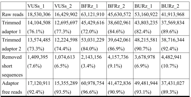
3.2 Adaptor removal efficacy...36

3.3 Aligner performance assessment...37

3.4 Cumulative mapping report...38

3.5 Annotation programs’ performance assessment...39

3.6 Total annotation report...40

3.7 Overall reads distribution within RNA families...41

3.8 Overall reads distribution within snoRNA families...44

3.9 Effects of sno_ext’s correction on data distribution...46

3.10 Addressing sequencing biases...49

4. Discussion...51

4.1 Preparation of the data prior to analysis...51

4.2 Mapping reads to the human genome...51

4.3 Comparison of annotation methodologies...53

4.4 Reads annotation and abundance assessment...54

4.5 Comparison between library preparation protocols...56

4.6 Biases of compositions and size...57

5. Conclusion...58

LISTOFTABLES:

Table 1: Characteristics of the most characterized snoRNAs ...9 Table 2: Summary of primers used in qPCR analysis for quantification of ncRNAs

transcripts’ abundance ...26

Table 3: Cutadapt summary of processed reads ...36 Table 4: Performance ranking summary of widely used mapping programs based on

literature ...37

Table 5: Adaptor free reads mapping summary to human genome (hg38 version 85) by

STAR and bowtie2 ...38

Table 6: Performance ranking summary of widely used annotation programs based on

literature ...39

Table 7: Read annotation summary by HTSeq and sno_ext ...40 Table 8: Correlation between quantification of ncRNAs from qPCR and sequencing in

LISTOFFIGURES:

Figure 1: H/ACA box snoRNAs structural elements and their associated core proteins ...3 Figure 2: C/D box snoRNAs structural elements and their associated core proteins

...4 Figure 3: Sequencing workflow from RNA extraction to sequencing ...12 Figure 4: Divisions of total RNA samples and labelling of sequencing sets ...23 Figure 5: Overview of a pipeline for the analysis of genomic sequencing data

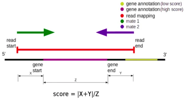
...27 Figure 6: Scoring schema for gene identification ...33 Figure 7: Global assessment of per base quality (phred score) in studied sequencing

datasets ...35

Figure 8: Global relative read expression (%) in CPM (left) and TPM (right) of the RNA families from the HTSeq analysis before corrections from sno_ext ...41 Figure 9: Global relative read expression (%) in CPM (left) and TPM (right) of the RNA families from the HTSeq analysis after corrections from sno_ext ...42 Figure 10: Relative expression (CPM) of the two snoRNAs families (H/ACA box & C/D box) in sequencing sets generated by size selection (VUSs) and the TGIRT method (B*Rz)

before correction by sno_ext ...44

Figure 11: Relative expression (CPM) of the two snoRNAs families (H/ACA box & C/D box) in sequencing sets generated by size selection (VUSs) and the TGIRT method (B*Rz)

after correction by sno_ext ...45

Figure 12A: Species abundance and read mapping according to different annotation protocols in the BURz set for HSPA8 and snoRNAs found within its introns

...46 Figure 12B: Ensembl genome view of gene annotations mapping to chromosomal position

of HSPA8 gene (Kb) ...46

Figure 13: Correlation between quantification of ncRNAs from qPCR and sequencing in

VUSs, BURz and BFRz sets ...45

Figure 14: Assessment of spike-ins composition as a factor affecting abundance (log2CPM) in the datasets generated by the TGIRT protocol ...49 Figure 15: Spike-ins length (nt) correlated to their distribution (log2CPM) in all sets produced through the TGIRT protocol ...50

LISTOFABBREVIATIONS:

Abbreviations: RNA species

RNA ribonucleic acid

caRNA chromatin-associated RNA

ncRNA non-coding RNA

mRNA messenger RNA

miscRNA miscellaneous RNA

snoRNA small nucleolar RNA

miRNA microRNA

tRNA transfer RNA

lincRNA long intergenic non-coding RNA

sdRNA small nucleolar derived RNA

sno-lncRNA Long non-coding RNA with snoRNA ends

rRNA ribosomal RNA

Datasets

BURz bacterial unfragmented ribodepleted BFRz bacterial fragmented ribodepleted VUSs viral unfragmented size selection

B*Rz bacterial ribodepleted

Techniques

qPCR quantitative polymerase chain reaction dNTPs deoxynucleotides triphosphate

Units

CPM count per million

TPM transcript per million

FPKM fragments per kilobase of exon per million reads mapped

Ct threshold cycle

Various

nt nucleotide

cDNA complementary DNA

PWS Prader-Willi Syndrome

ACKNOWLEDGEMENTS:

I would like to direct the most generous thanks I can muster to my supervisor Pr. Michelle Scott and Pr. Sherif Abou Elela for their guidance and support through my master’s. I also need to acknowledge the incredible work and energy invested in creating sequencing libraries by Sonia Couture from Pr. Abou Elela’s lab.

To the members of the Plateforme RNomique Genome Quebec, I wish to direct my deepest thanks for their assistance with the qPCR data acquisition and validation. I would like to insist on the importance of the members from Lambowitz’s lab, Douglas Wu and Ryan Nottingham which assisted as much as they could with the analysis. I am thankful to the Mammouth team at Sherbrooke University for their prompt assistance whenever there were issues with the nodes or a program that needed setting up.

Lastly, I would like to thank my family for tolerating my long absences and hectic behaviour through the years.

1. INTRODUCTION 1.1 General overview

1.1.1 Basic overview of snoRNAs

Small nucleolar RNAs, snoRNAs, are small non-coding RNAs (ncRNAs) species localized in the nucleolus and expressed throughout eukaryotes (Bachellerie, Cavaillé, & Hüttenhofer, 2002; Hoeppner & Poole, 2012). As small ncRNAs, snoRNAs’ length ranges, most often, between 60 and 200 nucleotides (nt) in humans, but can reach up to 1000 nt in yeast (Dieci, Preti, & Montanini, 2009). To add to this wide diversity of sizes, their genomic localization can also widely vary from organism to organism. Plant snoRNAs have their own transcriptional units while human snoRNAs are found to be preferentially, over 90% of them, encoded within introns, often of coding genes related to their functions (Dieci et al., 2009). The snoRNA presence within introns affects their biogenesis. Intron encoded snoRNAs are transcribed with their host simultaneously (Tycowski, Shu, & Steitz, 1993). The introns are excised from the pre-messenger RNA (pre-mRNA) into a lariat which the human debranching enzyme, hDBR1, linearizes (Petfalski, Dandekar, Henry, & Tollervey, 1998). At this point, the core proteins of the ribonucleoprotein (RNP) complex, are already bound to the snoRNA (Ballarino, Morlando, Pagano, Fatica, & Bozzoni, 2005). Most often this complex has a single associated function, referred to as canonical, the maturation of ribosomal RNAs (rRNAs). In that function, snoRNAs act as guide sequences that match by complementarity to target sequences found on the rRNAs. At this point, the ribonucleoprotein (snoRNP) complex bound to the snoRNA modifies chemically bases on the rRNA (Smith & Steitz, 1997). The type of modification is based on the protein complement attached to the snoRNA which, in turns, is dependent on the snoRNA family. The two families, H/ACA box snoRNAs and C/D box snoRNAs, are named after the conserved sequence elements, or boxes, found in each family.

1.1.2 H/ACA snoRNA structural features

The H/ACA box family is thus named for the presence of a H box (ANANNA, N being any nucleotide) and an ACA box. The guide regions, responsible for pairing with the target, are bipartite bulges of 10 to 20 nt distributed in the hairpins (Figure 1). The hairpins exhibit a high prevalence in base pairing making the H/ACA box snoRNAs a highly structured RNA family. The ACA box is highly conserved and located 3 nt from the 3’ end (Ganot, Caizergues-ferrer, and Kiss 1997; Reichow et al. 2007). This family accounts for the longer snoRNAs, with most of the members being between 120 and 160 nt, in terms of length. 1.1.3 H/ACA snoRNP biogenesis

The formation of the mature H/ACA snoRNP complex involves the assembly of a protein complex (Figure 1) composed of dyskerin (NAP57), SHQ1 and Naf1 (Hong Li, 2008; Li et al., 2011; Walbott et al., 2011). Dyskerin is the main catalytic unit of the complex, responsible for pseudouridylation of the target RNA species. SHQ1 binding to NAP57 prevents non specific RNA binding events and their improper linkage might be responsible for Dyskeratosis Congenita, a rare, congenital, progressive bone marrow failure disorder (Grozdanov, Fernandez-Fuentes, Fiser, & Meier, 2009). The Naf1, on the other hand, prevents an immature complex from having any activity. However, Naf1 is swiftly replaced by Gar1 to yield the active, mature ribonucleoprotein complex (RNP) (S Li et al., 2011). The RNP’s dyskerin binds to the snoRNA. A digestion by exonucleases of the 5’ and 3’ ends of the snoRNA template leaves the mature snoRNP. Once processed by the exonucleases, the overall structure adopted by H/ACA snoRNAs is that of a stem-hinge-stem with the H box located in between both stem-hinge-stems (Bachellerie, Cavaillé, & Hüttenhofer, 2002). The H box has been shown in recent studies to be dyskerin’s preferred binding site (Kishore et al., 2013).

1.1.4 C/D snoRNA structural features

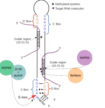
The second family, the C/D box snoRNAs, accounts for the most genes being close to a 5:2 ratio to the other family (Lestrade & Weber, 2006). The C/D box snoRNAs family is comprised of the smaller species, often ranging between 70 and 120 nt (Scott et al., 2012). The conserved sequence elements are the C and D boxes, however, unlike H/ACA snoRNAs, there are also often duplicates of theses sequences, though often degenerate, called C’ and D’ (Jorjani et al., 2016; Kiss-Laszlo, Henry, & Kiss, 1998; Samarsky, Fournier, Singer, & Bertrand, 1998). The C box sequence is RUGAUGA (R being a purine) while the D box sequence is CUGA. The C and D boxes are located toward the 5’ and 3’ ends of the molecule, respectively, whereas the C’ and D’ are closer to the middle (Figure 2). The guide regions are stretches of 10-21 nt, like in the H/ACA snoRNAs, however they do not share in the bipartite nature of the H/ACA snoRNAs guide regions. Both regions are found directly upstream from the D and D’ boxes (Cavaillé & Bachellerie, 1998). Further upstream, at the pairing between the C box and D box, there is the kink-turn, also labelled k-turn, which is created from two consecutive G-A pairings. This non Watson-Crick pairing results in a sharp turn in the RNA’s structure (Henras, Dez & Henry, 2004).

Figure 1: H/ACA box snoRNAs structural elements and their associated core

proteins. H/ACA box snoRNAs have two conserved boxes, H box (ANANNA) and ACA box (ACA). Two guide regions pair up with their target RNA molecules. The assembly of a mature H/ACA snoRNA requires a full complement of proteins here depicted are NOP10, L7Ae, Dyskerin, Naf1, SHQ1 and Gar1.

1.1.5 C/D snoRNP biogenesis

The C/D snoRNP biogenesis is similar in many ways to the step-wise assembly of the H/ACA box snoRNAs (Figure 2). The first step is the formation of a protein complex. The 15.5K protein, analogous to the snu13p found in yeast, forms a complex with NOP58 (Bizarro et al., 2014). The 15.5K protein starts the folding by binding the C and D boxes which causes the creation of the k-turn (Watkins et al., 2000; Watkins, Dickmanns, & Luhrmann, 2002). NUFIP, analogous to the yeast’s rsa1p, is then bound to the 15.5K protein and prevents the complex from carrying out its activity, akin to Gar1 for the H/ACA snoRNAs. NUFIP is also responsible for enhancing the binding of the complex to the snoRNA component, and the recruitment of the chaperone HSP90-R2TP (Boulon, Bertrand, & Pradet-Balade, 2012; McKeegan, Debieux, Boulon, Bertrand, & Watkins, 2007; Rothé et al., 2017). Fibrillarin and then, NOP56 sequentially bind to the complex and release the NUFIP factor effectively yielding the mature C/D box snoRNP. The previously mentioned k-turn is essential as it serves as an assembly and recruitment point for the fibrillarin complex (Henras et al., 2004).

Figure 2: C/D box snoRNAs structural elements and their associated core proteins. C/D box snoRNAs have two conserved boxes, C box (RUGAUGA) and D box (CUGA). Two guide regions pair up with their target RNA molecules. A k-turn is located upstream of the C box. The assembly of a mature C/D snoRNA requires a full complement of proteins here depicted are NOP56, NOP58, fibrillarin, 15.5K and NUFIP.

1.1.6 snoRNA canonical function

The function that is most often associated with snoRNAs is the maturation of other RNA species, most often rRNA, but also tRNAs, snRNAs and other snoRNAs, through chemical modifications (Kawaji et al., 2008; Kishore et al., 2013). As previously mentioned, the type of modification depends on the core proteins associated to the snoRNPs which, is itself dependent on the family of snoRNA. The H/ACA box family is responsible for the pseudouridylation of its targets through the protein dyskerin. The guide regions are located on both stems. This, in turns, explains why the pseudouridylation occurs 14-15 nt upstream from either the H or ACA box (Ganot, Bortolin, and Kiss 1997). The modification is an isomerization of the uridine base. The most noteworthy property of pseudouridine, compared to other bases, is the presence of the hydrogen bond donor (Ge & Yu, 2013). On the other hand, the C/D box family is associated to its fibrillarin’s methylation activity. The methylation occurs on the 2’ hydroxyl group of the ribose (Cavaillé & Bachellerie, 1998; C. M. Smith & Steitz, 1997). The target sequence is bound to the snoRNA’s guide regions, 5 nt upstream of both the D and D’ boxes (Tycowski, Smith, Shu, & Steitz, 1996). The presence of two guide regions in C/D box snoRNAs indicate that up to 2 substrates can be recognized simultaneously (Kiss-László, Henry, & Kiss, 1998). However, not all snoRNAs fall within these neatly defined functions. A sizeable proportion, ~ 42% of snoRNAs, were reported, back in 2015, to lack a clearly defined function because of a lack of identifiable target (reviewed in Dupuis-Sandoval, Poirier, and Scott 2015). They were labelled orphan snoRNA. A recent study examined past high-throughput data and 2’-O-methyl profiles to put this number down to 17 % (Jorjani et al., 2016).

1.1.7 Orphan snoRNAs

Orphan snoRNAs are a subset of snoRNAs lacking a clearly defined target to modify through either methylation or pseudouridylation. Recent studies have assigned targets to four orphan snoRNAs through conservation of evolutionary homology in target sequences (Kehr, Bartschat, Tafer, Stadler, & Hertel, 2014) and identified modification sites that had, until then, been ignored. However, even after removing those 4 predictions, 143 snoRNAs species remain lacking a defined function. In recent years, through the advent of wide spectrum methodologies of analyses such as next-generation sequencing (NGS) technologies, photoactivable ribonucleoside-enhanced crosslinking and immunoprecipitation (PAR-CLIP), and mass spectrometry, big data has been able to shed light on unexpected phenomenon with increased statistical significance (Hafner et al., 2010; Kishore et al., 2013). One such unexpected discovery was that snoRNA can be bound to proteins other than the core RNPs. An increased diversity of interactors is relevant, as it can be interpreted as a wider range of functions in which snoRNA are potential actors. The alternative snoRNA’s roles put forward, at this point in time, are linked to resistance to lipotoxic shock, chromatin unwinding and, to some extent, splicing. The first method in which snoRNAs can act unusually, is by modifying targets that are not normally attributed to them. When looking at the species bound to the core C/D box RNPs, unlikely species were identified as modified. These ncRNAs species were snoRNAs, snRNAs, tRNAs, but, perhaps more interestingly, vault RNAs, 7 SK and 7 SL (Kishore et al., 2013).

1.2 non-canonical functions

As mentioned before, the advent of NGS technologies has allowed to generate massive amount of data about expansive biological systems. These methods are unlike those of the past where molecules had to be studied individually. This phenomenon accounts for the limited number of snoRNAs with an appreciable depth of characterization. NGS technologies have also allowed to characterize RNA species found within individual cell compartments and organelles. This ability to segregate and characterize compartments negated the common perception that the cytoplasm did not contain snoRNAs (Holley et al., 2015).

1.2.1 snoRNA and stress responses

As touched in the earlier paragraph, the lack of wide spectrum analysis methods meant that entire species were not studied for decades. SNORD32A, SNORD33 and SNORD35A, are such molecules, all localized within the introns of RPL13A. They were reported in 1996, however until 2011, their implication in lipotoxicity resistance remained a mystery (Michel et al., 2011; Nicoloso, Qu, Michot, & Bachellerie, 1996). Knockdown of the host gene and, therefore, its associated snoRNAs induced a resistance to lipotoxic and oxidative shocks (Michel et al., 2011). The potential of snoRNAs as agents of metabolic stress was further demonstrated when a RNA immunoprecipitation coupled with sequencing (RIP-seq) detected an increased snoRNA representation on the protein kinase RNA-activated (PKR), a protein involved in the stress response, when a cell is exposed to metabolic stress (Youssef et al., 2015). As such, the human stress response seems intricately linked to snoRNAs.

1.2.2 snoRNA and chromatin

SnoRNAs are used for signalling in other organisms than humans. In Drosophila cells, RNA bound to Df31 is responsible for maintaining the open “unwound” state of chromatin (Schubert & Längst, 2013). RNA molecules bound to chromatin are referred to as chromatin-associated RNAs or caRNAs. caRNAs were shown to be predominantly H/ACA snoRNAs (Schubert et al., 2012).

1.2.3 snoRNA and splicing

Classically, the sites targeted by snoRNA were located on ncRNAs and pre-rRNA, however, pulldown experiments on snoRNAs’ interactors show that snoRNAs bind sites found on mRNA (Gumienny et al., 2016). However, the same study demonstrated that these sites fail to be methylated. This absence of modification might allude to a mode of action that falls outside the canonical definition. Though this is a single example, other instances of snoRNAs acting on mRNA exist. The well characterized snoRNAs species SNORD116 and SNORD115 are known to be major actors in the Prader-Willi Syndrome (Kishore & Stamm, 2006; Peters, 2008; Skryabin et al., 2007). Recently, SNORD115 was put forward as modulating the expression of SNORD116. SNORD115 affects the pre-mRNA splicing of the serotonin receptor 2C on its exon Vb, though the exact method by which splicing of the transcript remains unclear (Kishore & Stamm, 2006; Kishore et al., 2010). SNORD116, on the other hand, does not appear to affect splicing, but rather its deletion causes a change in the expression level of certain mRNAs (Cavaille, 2017; Falaleeva, Surface, Shen, de la Grange, & Stamm, 2015). The SNORD116 family was also reported to form long non-coding RNAs derived from sequences between two snoRNAs being incorporated into snoRNA long ncRNAs, sno-lncRNAs. The deletion of 5-6 Mb from the locus containing sno-lncRNAs is present in PWS (McCann & Baserga, 2012). Furthering the link between splicing and snoRNAs, these sno-lncRNAs were found to bind RBFOX2 (also called RBM9), a member of the FOX family, which are regulators of alternative splicing (Yin et al., 2012; Zhang et al., 2014). The physiological effects of the sno-lncRNA deletion on the mice are consistent with PWS. The trait common to PWS are low birth weight, followed by increased body weight gain in adulthood, increased energy expenditure and hyperphagia (Qi et al., 2016). On the other end of the spectrum, smaller fragments of snoRNAs have been described in the literature (Falaleeva & Stamm, 2013; Kawaji et al., 2008; Taft et al., 2009).

Those snoRNA derived species (sdRNAs) are between 18 and 30 nt, meaning that they are closer in length to miRNAs than to the full snoRNA template (Brameier, Herwig, Reinhardt, Walter, & Gruber, 2011). Their biogenesis is, like miRNAs’, dependent of Dicer, but, unlike miRNAs’, it is independent of Drosha/ DGCR8. These sdRNAs are implicated, in a similar way to miRNAs, in the silencing pathways (Brameier et al., 2011; Scott & Ono, 2011). One such sdRNA comes from the processing of SCARNA45 (Ender et al., 2008). Similar cases of known miRNAs originating from snoRNA precursors include let-7g, mir-140, mir-151 and mir-16-1 (Ono et al., 2011; Scott, Avolio, Ono, Lamond, & Barton, 2009).

1.3 Categorizing and detecting snoRNAs

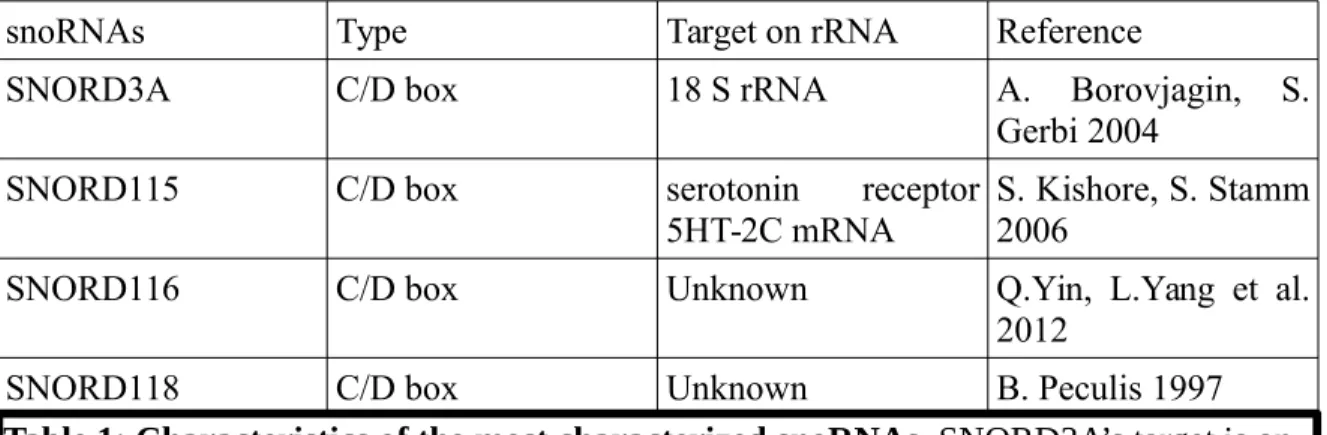
1.3.1 Improving on snoRNAs’ characterization through a global sequencing approach The widespread usage of NGS has only recently taken roots. In the 1990s and early 2000s, snoRNAs were studied individually and a sizable quantity of genetic material had to be extracted in order to give a fair representation. The laborious nature of the process meant that the analysis of the most abundant species was favoured. As such, SNORD3A, SNORD118 and species with special relevance to diseases such as PWS’s SNORD115 and SNORD116 were studied early on (Kass, Tyc, Steitz, & Sollner-Webb, 1990; Tyc & Steitz, 1989). By the same process, low abundance and tissue-specific snoRNAs were ignored (Table 1).

snoRNAs Type Target on rRNA Reference

SNORD3A C/D box 18 S rRNA A. Borovjagin, S.

Gerbi 2004

SNORD115 C/D box serotonin receptor

5HT-2C mRNA S. Kishore, S. Stamm2006

SNORD116 C/D box Unknown Q.Yin, L.Yang et al.

2012

SNORD118 C/D box Unknown B. Peculis 1997

Table 1: Characteristics of the most characterized snoRNAs. SNORD3A’s target is on 18S rRNA while SNORD115’s target is located on the serotonin receptor 5HT-2C exon V. SNORD116 and SNORD118 do not have any identified rRNA target.

Until a few years ago, the technical constraints of the past were reflected in the absence of big data on which a global portrait of snoRNAs could be made. Today, the relatively low cost, speed and ease at which sequencing can be performed is responsible for the growing abundance of small ncRNAs datasets. Nonetheless, even with the massive quantity of data, the snoRNAs are not well detected. In most sequencing sets, snoRNAs are not perceived at a sufficient depth to allow characterization. There is also the added issue that the ratio between both families is always skewed toward an overwhelming, >90%, representation of the C/D box snoRNAs species (Deschamps-Francoeur et al., 2014; Kishore et al., 2013). The low number of detected H/ACA box snoRNAs limits our ability to categorize and study an important portion of all snoRNAs. Furthermore, an additional piece of the puzzle is still missing to properly judge the properties of snoRNAs, a way to compare the species to their host and to the full spectrum of possible interactors.

As of late, the identification of snoRNAs’ implications in biological processes as diverse as splicing or lipotoxicity resistance have opened the possibility of other hidden partnerships between interactors that until now hadn’t been considered. To identify such interactions, the snoRNAs and their potential partners need to be compared to each other and with the base expression level to theorize how one modulates the expression of the other. Protein-coding genes combined with snoRNAs genes profiles would allow to infer partners to snoRNAs in their non canonical functions. As a consequence, more depth of data, enough to encompass snoRNAs and protein-coding genes, is required. To summarize, the data has to be broad enough to capture snoRNAs and their interactors while being deep enough that statistical inference remains a possibility. As such, these specifications leave only sequencing as an option for a semi-quantitative analysis. The entire RNA species within a cell represents very heterogeneous data in terms of length, base composition and structure. The sequencing protocol has to be likewise broad and permissive to capture all the fluctuations in the snoRNAs’ length and abundance.

1.3.2 Introduction to sequencing:

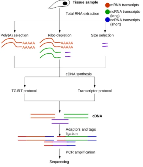
The first step in the needed RNAseq workflow consists of a proper isolation of the RNA species chosen for quantification through a RNA extraction protocol. The method by which RNA species are extracted and selected affects the overall scope of the study. The frequently used protocols available to extract and enrich RNAs are poly(A) selection, ribo-depletion, and size selection (Figure 3) (Zhao et al., 2014).

1.3.2.1 Poly(A) selection

Poly (A) capture protocols rely on poly (T) oligomers to affix the adaptor unto the second strand template through the amplification process (Chang, Lim, Ha, & Kim, 2014; Zhao et al., 2014). This creates a bias as only species with polyA are detected which are mostly mRNAs (Cui et al., 2010). The coverage of mRNA is also subject to a bias against the 3’ extremity as it often has homopolymeric repeats (Chang et al., 2014). Human snoRNAs are predominantly encoded within intronic regions and do not have polyadenylated tails (Dieci et al., 2009). As such, human snoRNAs, among other ncRNAs, have been found to be very poorly represented in datasets generated through poly(A) selection protocols (Zhao et al., 2014).

1.3.2.2 size selection

The second method, size selection, is most often used to sequence miRNAs (Head et al., 2014). This protocol isolates small RNA species based on their molecular weight through a glass fiber column purification. The column purification allows to extract species with less than 200 nt (Shingara et al. 2005). These species are then amplified through PCR cycles and sequenced. This selection, however, removes the longer protein-coding and ncRNAs transcripts (Sheng Li et al., 2014).

1.3.2.3 Ribo-depletion:

Ribosomal RNAs are often the most abundant RNA species within untreated samples. It was estimated that rRNA species can represent 90% of the detected species (O’Neil et al. 2013). Often rRNA can very effectively be removed of RNA samples through ribo-depletion (Conesa et al., 2016). Ribo-ribo-depletion relies on the hybridization of probes to rRNAs followed by precipitation on magnetic beads (O’Neil et al., 2013).

Figure 3: Sequencing workflow from RNA extraction to sequencing. The first step is to extract the total RNA from the tissue sample. The RNA is then further selected through various isolation protocols differentiating between mRNAs, longer and smaller ncRNAs. The RNA is then put through a PCR cycle which results in cDNAs. The adaptors and tags are added to the cDNA. The cDNA is then amplified either through the standard Transcriptor protocol or the TGIRT protocol before being sent for sequencing.

Extraction is usually followed by amplification of the RNA species to ensure detection by the sequencer. The result is complementary DNA species to the isolated RNA species on which two adaptor sequences and a tag were affixed through a step of adaptor ligation. These steps finalize the preparation of an appropriate library.

1.3.3 Injection of spike-ins

As an extra step, it is possible to add fixed amounts from a calibrated solution of spike-ins. These small RNAs do not have any match on the human genome. As such, they can be safely detected without the risk of being confused for another species. The spike-ins can be used as a means to estimate the presence biases in lower sizes molecules (Risso, Ngai, Speed, & Dudoit, 2014). The ERCC spike-ins are sold as 2 cocktails of molecules of varying length and base composition. ERCC spike-ins are mixed with the library samples. The concentration of each cocktail is equal and conserved variations in the perceived count after sequencing could indicate biases in the sequencing methodology (Locati et al., 2015). They can also be used to normalize species found below 100 nt, by adjusting count by a factor equal to the detected spike-ins (Nottingham et al., 2016).

The completed libraries are sent to an external site for sequencing. There, the cDNA is pooled, then bound to a flow cell by complementarity between a primer on the surface of the cell and the incorporated adaptor. Once binding to the flow cell is done, the species are amplified to create detectable clusters in a step named bridge amplification. A polymerase, nucleotides and buffer are added to the flow cell’s environment to initiate the amplification process. The DNA species bridging is done by complementarity between the free adaptor sequence and a second complementary primer on the flow cell. The bridged DNA’s complement sequence is transcribed by the polymerase. This process is repeated multiple times to create a cluster.

1.3.4 Sequencing-by-synthesis

The clusters are sequenced by sequentially adding bases with fluorescent dyes. The fluorescent dyes are various chromophores of specific wavelength which are freed upon binding to their complement base. These signals are intercepted by the sequencer. The sequencing apparatus attributes a quality score based on the purity and strength of the signal. This score takes the form of a Phred score, a logarithm based measure of certainty for the nature of the base sequenced. The process, as mentioned previously, is sequential, that is to say, for each base on the target sequence, bases are added until a match is found and then the following base goes through the same process. However, as bases are sequenced, the signal becomes muddled because unsuccessful reactions cause a lag in synchronization which, ultimately, accounts for a drop in the base calling confidence (Fuller et al., 2009).

1.3.4.1 Paired-end sequencing

A way to counteract the aforementioned decay in base calling confidence is to rely on paired-end sequencing. Paired-end sequencing is based on a set of complementary adaptors ligated to 3’ and 5’. The presence of complementary adaptors yields both forward and reverse strands which is also done in the single-end standard protocol, however unlike the former, the reverse strand of the target sequence is conserved for further analysis.

1.3.4.2 Bypassing inherent sequencing biases

The second hurdle in generating data as unbiased as possible lies in the use of the commercially available reverse transcriptase, Transcriptor. When creating the libraries, the use of the viral reverse transcriptase has been shown to lower the representation of highly structured RNA species such as tRNAs, snoRNA and snRNAs (Nottingham et al., 2016; Zheng et al., 2015). This issue would affect our estimation of snoRNA abundance and affect every conclusion reached. An encouraged alternative to the viral reverse transcriptase was the thermostable group II intron reverse transcriptase, also known as TGIRT.

1.3.5 Group II introns

Group II introns are a family of bacterial mobile retroelements with intron-encoded reverse transcriptase and an autocatalytic RNA (Lambowitz & Zimmerly, 2004; Truong, Sidote, Russell, & Lambowitz, 2013). Group II introns have also been identified in mitochondrial’s, chloroplast’s, plants’ and fungi’s genomes. However, this family is absent of nuclear genomes (Lambowitz & Belfort, 2015). The group II introns’ ability for retrohoming and retrotransposition has been linked with the appearance of spliceosomal introns, retrotransposons and telomerase. The autocatalytic component is responsible for the insertion of his cDNA into the host genome (Enyeart, Mohr, Ellington, & Lambowitz, 2014; Nottingham et al., 2016; Zheng et al., 2015). However, the most pertinent component of group II introns as far as sequencing technologies are concerned is the reverse transcriptase (Mohr et al., 2013). The RT, under normal condition, synthesizes the complement DNA (cDNA) while also having endonucleolytic capabilities (Lambowitz & Zimmerly, 2004; Nottingham et al., 2016). Structurally, the RT is similar to retroviral RTs with an extra conversed block and distal binding sites (Blocker, Mohr, Conlan, & Qi, 2005; Lambowitz & Belfort, 2015). Both the RNA and RT components can work independently from one another. This modularity, ultimately, means that for the purpose of creating sequencing libraries, the RT can be isolated from the rest of the group II intron complex (Enyeart et al., 2014). TGIRT libraries were shown to represent quite aptly tRNAs when compared to the standard illumina sequencing protocol (Zheng et al., 2015). The hypothesis of this study is that the use of the TGIRT protocol on a new generation of the illumina HiSeq sequencer would ensure a better depth and representation of snoRNAs. 1.3.6 Pipeline for the analysis of total RNAs

The analysis of the sequencing data, in itself, raises a number of problems since most methods make assumptions about the nature of the data. As such, for an analysis pipeline to be fitting, a minimum of time must be spent examining the tools available. The standard bioinformatics workflow to examine NGS data begins with an examination of the quality of the sets (Conesa et al., 2016).

Following that assessment, the data is treated to remove bases corresponding to non-genomic sequences (tags, adaptors and multiplexes) and low quality segments found within reads as the practice has been found to improve overall data quality (Shendure et al., 2008). Once the reads’ quality ascertained, the process of mapping the reads to the genome through an aligner is carried out. The final step is to associate the genomic ranges found to map to reads to their corresponding genes and transcripts (Conesa et al., 2016).

1.3.7 Quality assessment

Quality assessment serves as a preliminary examination of the composition of the NGS sets. The program FastQC computes helpful metrics such as the sequence’s base composition, GC content, unknown base content, duplication rates, length and quality scores (Andrews, n.d.). Different protocols to create libraries come with predicted biases. Isolation of variants of a few transcripts results in a fail of the sequence duplication analysis. The presence of adaptors within the reads fails the analysis of the Kmer content. Such scenarios can be brought up for each category. As such, implementation of checks throughout the NGS data’s treatment are privileged.

The first step before the analysis of the reads is to remove all non genomic segments and reads that would, otherwise, impair proper analysis. This step incorporates multiple processes, the removal of adaptor sequences from the reads, the removal of small reads that could map at multiple locations and the trimming of the lower quality portions of the reads (Martin, 2011; Shendure et al., 2008). Removal of the adaptors is done, normally, by a flexible regular expression that matches the given sequence and returns the reads free of the adaptors.

Trimming is performed by scanning the reads from the end of the reads’ sequences and removing all bases falling below a certain threshold, often a Phred score of 20 or 30. Both of the previous steps can be implemented in the same tool offering the possibility of executing both procedures simultaneously (Martin, 2011).

Once all non-genomic contamination has been removed, the reads are ready to be mapped to the genome. Multiple mapping strategies and algorithms have been implemented into stand-alone programs available to all (Bray, Pimentel, Melsted, & Pachter, 2016; Conesa et al., 2016; Dobin et al., 2013; Havgaard, Torarinsson, & Gorodkin, 2007; Kent, 2002; Kim et al., 2013; Langmead & Salzberg, 2012; Larkin et al., 2007). However, the principle remains the same. Two strings of characters are compared, one being the read, the other the reference, chromosome or genome to see where the best match for the read is located on the reference sequence. Alignment algorithms are designed to either support local or global alignment with a few programs allowing for both (Langmead & Salzberg, 2012).

Global alignment, as opposed to local alignment, requires the mapping of both ends of the supplied sequence to the target sequence. The first working global alignment method used for biological purposes used the Needleman-Wunsch algorithm (Needleman & Wunsch, 1970). Through heuristics, this method was improved and remains used today to find the best global alignment (Kent, 2002). However, the Smith-Waterman local alignment algorithm, postulated in 1981, found popularity shortly thereafter (T. F. Smith & Waterman, 1981). These methods were pushed forward with the creation of the first sequencing-by-synthesis machines from Solexa, now owned by Illumina, and a new wave of alignment algorithms were designed. At that time, the early 2000’s, tools like MAQ, BWA, SOAP and BLAT were created (Heng Li & Homer, 2010). BWA and SOAP relied on the Burrow-Wheeler Transform to improve on memory usage by compressing the index (Heng Li & Durbin, 2009). Further recent improvements on the index building and alignment principles have yielded critical advances.

1.3.8 Differences between aligners

The main differences in protocols come from the choice of alignment software and the way in which reads are annotated afterwards. Today, with the recent popularization of NGS, sequencing data has become abundant and the methods to align reads has become equally varied. The most widely used and documents alignment software are Splice Transcripts Alignment to a Reference (STAR), Tophat2, Bowtie2 and Kallisto (Conesa et al., 2016). The first candidate, Kallisto, is a software written in python with the core aligner in C++ (Bray et al., 2016). The main quirk from Kallisto is the lack of actual alignment for each base or k-mer, rather it relies on pseudoalignment. The transcriptome is extracted from a fasta file and a De Brujin graph free of redundancy is built from k-mers as an index (Bray et al., 2016). The reads are then used as error-free paths which means mismatches between reads and transcriptome are disregarded entirely. The gene count utilizes an expectation-maximization (EM) algorithm. The reliance on a single De Brujin graph reduces the requirements in terms of CPU usage compared to other programs. Kallisto is also much faster as it does not perform complete alignments for each base. However, Kallisto cannot perform transcript discovery and extensions are hard to estimate.

Bowtie2 is an aligner based the use of full text minute (FM) index and the Burrow-Wheeler Transform. It is written in C++ (Langmead, 2013). This aligner is widely used for its ability to tolerate gap regions and perform local alignments. The biggest CPU usage from bowtie2 comes from its FM index which takes a bit more than 3 GB for the human genome. Even if the memory footprint is non negligible, any modern laptop should be able to allocate this much memory and its speed of execution is also quite respectable, being faster than the Tophat2 (Langmead & Salzberg, 2012).

The next alignment software is Tophat2, a splice junction aware program written in python and C++. Tophat2 uses bowtie2’s aligner, but implements routines to take splicing of mRNA into account (Kim et al., 2013). A series of improvements have been made since the initial release of Tophat to reduce the number of core hour needed to produce the alignments. However, it still lags behind Kallisto and STAR while its alignment is quite similar to the one created by STAR.

STAR is a C++ alignment program that aimed at improving the mapping speed while allowing for new junctions discovery. It does so by looking up seeds and, in a second step, scoring them. The seed search portion relies on the Maximum Mappable Length (MMP) or mapping iteratively the longest contiguous segments of a read. The second step unites the various possibilities of seeds together and using a local alignment grading scheme assigns scores to them. The higher score is conserved as the best match and returned. STAR achieved a multiple fold faster speed of mapping than Tophat2 on simulated data (Dobin et al., 2013).

Alternatively, Cufflinks can be used to analyze RNA sequencing sets. The suite of programs Cufflinks has been created in 2009 by the Trapnell lab and remains to this day a widely used pipeline. It was designed to primarily handle sets covering the exons and protein-coding regions of the genome. This particularity is its strength since Cufflinks relies on normalization factors used specifically in protein-coding analysis, such as, FPKM (Trapnell et al, 2012). This method does not agree with comparative studies between sets because it does not normalize to negate sequencing depths differences (Conesa et al, 2016). Other normalization factors commonly used are CPM or TPM. The main difference between both method lies in TPM’s adjustment for the transcript’s length. Nonetheless, both TPM and CPM retain the last step of normalizing for sequencing depth. In turns, the last step allows comparison between individual counts as the sum of an experiment will always add up to a million. Ultimately, this makes CPM and TPM more relevant to a comparative study. Furthermore, the nature of our analysis, where sets are principally composed of small RNAs, made cufflinks and associated software ill-suited because it removed the possibility to account for the mobile nature of small ncRNAs. These preceding documented reasons excluded Cufflinks from any enquiry.

1.3.9 Differences between annotation strategies

Once the reads are mapped, the following step would be to assign the reads to the genes. The most popular methods are HTSeq, RSEM, bedtools multicov. The first program, RSEM, is written mainly in C++. RSEM’s annotation process is anchored on an iterative fitting method called Expectation-Maximization (Kanitz et al., 2015). RSEM provides plenty of useful feedback, such as the various gene counts after normalization. The output takes the form of the gene identification, the transcripts identifications, the length, the expected count, the TPM and the FPKM.

Bedtools is a platform written in C++ for the analysis of mapped genomic data. It offers a suite of scripts useful to study the various genomic intervals returned within the BAM files (Quinlan & Hall, 2010). Multicov, one of the scripts, uses a gtf annotation file to return the number of overlaps between reads and each of the features. The information returned through this process is composed of the reference’s name, start position, end position and the reads count mapping to the interval.

HTSeq is a platform for executing simple manipulations on genomic data. The platform and its associated scripts are entirely written in python. It was designed to be adapted to fit the user’s needs. Within HTSeq, the script HTSeq-count provided a general template of the annotation process. The script allowed for the use of paired-end sequencing and provided ample information pertaining to its usage (Anders, Pyl, & Huber, 2015). The HTSeq output is the gene name and the associated reads count.

1.4 Objectives

As mentioned before, the snoRNAs species have, thus far, not been properly characterized because of the methods’ limitations. However, with the advent of sequencing technologies, new protocols are available. Those protocols have yielded new insight into snoRNAs’ alternative roles, however those studies examined proteins that were not known snoRNAs interactors and are, by extension, serendipitous events. The limited spectrum of molecules surveyed forbids a further look at the fluctuations of snoRNAs populations. As such, the first objective of our study is to find the most reliable sequencing protocol for the detection of RNAs species, specifically snoRNAs. To this end, the TGIRT protocol known for its ability to capture small, highly structured RNA species’ profiles like the tRNAs will be pitted against the more conventional protocols. It is our team’s hypothesis that the abundance profiles given by the TGIRT protocol will be a fairer representation of snoRNAs’ abundance than any other alternative. The second objective is to construct a bioinformatics workflow able to detect qualitative and quantitative shifts in the snoRNAs. This pipeline would allow to hazard an hypothesis concerning alternative functions and interactors of snoRNAs.

2. MATERIALAND METHODS

2.1 Generation of genomic data 2.1.1 Cell culture and transfection

The analysis and use of non simulated genomic data was invaluable to assess the presence of biases in next generation sequencing protocols. Cell types that had already been characterized would have to be used to ensure that variations from past experiments could be validated. As such, the cell type SKOV3ip1 was selected as the members of the lab personnel had experience in handling, cultivating and past datasets were readily available. SKOV3ip1 is an ovarian adenocarcinoma cell type. The cells were grown in DMEM/F12 (50/50) medium with 10% fetal bovine serum and 2mM L-glutamine. Cells were seeded at 350 000 cells per well.

2.1.2 RNA extractions

Total RNA extractions were carried out based on the protocol provided by the manufacturer, Qiagen. Following extraction, RNA integrity was confirmed by Agilent 2100 Bioanalyzer. All samples were brought to a volume of 11 μl. Random hexamers, dNTPs and RnaseOUT from Invitrogen were added, bringing the total volume of each sample to 20 μl. All samples were put through a reverse polymerase chain reaction (RT-PCR) using Transcriptor Reverse Transcriptase from Roche Diagnostics. Reverse transcription was carried out at 55 °C which is well within the optimal temperature range of 45-60 °C.

2.1.3 Library preparation and sequencing

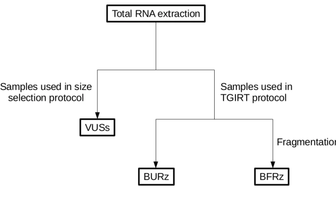
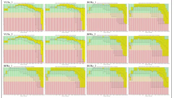
Two batches of samples were prepared, the first in the summer of 2013, was made of 8 samples, however only 2 replicates (VUSs_1 & VUSs_2) are relevant to this analysis. While the second batch was prepared during the winter of 2016 and was made of 4 samples (BURz_1, BURz_2, BFRz_1 & BFRz_2) (Figure 4). The former batch of libraries, VUSs_1 and VUSs_2, was prepared by size selection using the mirVana toolkit by following the instructions provided by the manufacturer, ThermoFisher Scientific. Small non-coding RNA (ncRNAs) species with low molecular weight (<200 nt) were isolated.

The isolated samples were put through the TruSeq Small RNA Sample Prep kit from Illumina following the protocol provided by the manufacturer. The isolated cDNA was ligated to 3’ and 5’ adaptors included within the kit’s materials. The cDNA was reverse transcribed and amplified through PCR cycles. The reverse transcription ensured that only species with both adaptors properly ligated were amplified.

The following step, amplification, was required to generate a signal strong enough to be interpreted by the sequencer. Amplification was achieved by incubating the DNA samples in a thermal cycler through a 11 cycles PCR reaction. Verification of the samples integrity through Agilent 2100 Analyzer attested of the libraries’ purity.

Figure 4: Divisions of total RNA samples and labelling of sequencing sets. Following a total RNA extraction, the samples were subdivided between those subjected to the library preparation for size selection protocol and those put through the TGIRT library preparation protocol. The TGIRT samples are further subdivided between those that underwent a step of fragmentation and those that did not.

The libraries, VUSs_1 and VUSs_2, were sent to McGill’s and Genome Quebec Innovation center’s sequencing platform to be sequenced on a HiSeq2000 sequencer from Illumina. The two samples of interest were paired-end sequenced at a read length of 100 nt and their depth are 18.5 and 16 M reads. The datasets are stored on NCBI’s GEO portal under the accession number GSE55946.

The latter batch of libraries, BURz_1, BURz_2, BFRz_1 & BFRz_2, was prepared according to the specifications provided by Pr. Alan Lambowitz from the University of Texas (Nottingham et al., 2016). After each of the following steps, purification was carried out using Pr. Lambowitz’s modified version of the Zymo RNA Clean & Concentrator protocol. The total RNA samples were ribodepleted using the RiboZero Gold kit from Illumina following the protocol provided by the manufacturer. The samples were mixed with a supplied spike-ins cocktail to varying ratios described by Pr. Lambowitz. The ERCC spike-ins cocktails were added, 2 µL to a 5 µL volume of the aforementioned total RNA sample (Nottingham et al., 2016). The 4 samples were subdivided. Half, BFRz_1 and BFRz_2, were fragmented using an NEBNext Magnesium RNA Fragmentation Module from New England Biolabs at a temperature of 94°C for a duration of 7 minutes. Afterwards, all of the four samples, BURz_1, BURz_2, BFRz_1 & BFRz_2, were treated with T4 polynucleotide kinase phosphatase from Epicentre.

The T4 polynucleotide kinase ensured that samples would be free of 3’ phosphates and 2’, 3’ monophosphates which have been previously described to prevent the TGIRT-III’s ability for template switching (Mohr et al., 2013) and adopted into Pr. Lambowitz’s protocol. All of the 4 samples, BURz_1, BURz_2, BFRz_1 & BFRz_2, were put through reverse transcription with 1μM TGIRT-III RT from InGex, LLC and 5′ AppDNA/RNA Ligase from New England Biolabs for a duration of 15 minutes at a temperature of 60 °C and amplified for 12 cycles in a thermal cycler. Amplification was carried out as previously described (Nottingham et al., 2016). Sequencing for the 4 samples, BURz_1, BURz_2, BFRz_1 & BFRz_2, was done on site at the University of Texas’s Genomic Sequencing And Analysis Facility in Houston on a Hiseq 4000 from Illumina. Reads were paired-end at 150 nt and each dataset contains approximately 30 millions reads.

2.1.4 Quantitative Polymerase Chain Reaction (qPCR)

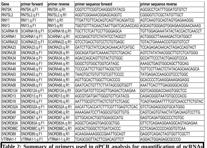
qPCR were run in house at the Plateforme RNomique Genome Quebec found at the address (http://rnomics.med.usherbrooke.ca/). A list of protein coding and snoRNA genes was submitted to the members of the Plateforme Rnomique. Primers were designed based on the lack of sequence repetition and folding of the targeted RNA molecule (Table 2). Total RNA was extracted from SKOV3ip1 cells using TRIzol from Invitrogen with chloroform following the manufacturer’s protocol. The recovered RNA was purified using the Rneasy Mini Kit column from Qiagen. A DNAse treatment was carried out as per the manufacturer's instructions. RNA integrity was confirmed by Agilent 2100 Bioanalyzer.

The extracted RNA was put through reverse transcription using 1.1 µg from the total RNA with Transcriptor reverse transcriptase, random hexamers, dNTPs from Roche Diagnostics and 10 units RNAseOUT from invitrogen. Forward and reverse primers were suspended in 20-100 µM Tris-EDTA solution from IDT and diluted as a primer pair to 1 µM in Rnase Dnase free water from IDT. The PCR reactions were carried in 10 µL in a 96 well plates on a CFX-96 thermocycler with a 5 µL volume of 2X iTag Universal SYBR Green Supermix, 3 µL of cDNA, and 2 µL from the previously mentioned primer pair solution. The thermocycler and iTag solution came from BioRad. The thermocycler was brought to 95 °C for 3 minutes and then, the cycling conditions were set as 50 cycles of 15 seconds at 95 °C, followed by 30 seconds at 60 °C, and then 30 seconds at 72 °C. Relative expression levels were assessed using the qBASE framework (Hellemans, Mortier, De Paepe, Speleman, & Vandesompele, 2007). No-template runs were carried out as negative controls (Brosseau et al., 2010).

2.2 Analysis of genomic data

Data obtained through sequencing methods has to be collected, and analyzed (Figure 5). The collection and further treatment is designed to remove and identify potential biases in the experimental design. Collection of the data was done through the set up of a server dedicated to data storage. The transfer was done through SSH protocol. Once the transfer was completed, a checksum verified that the data retained its integrity. The data was transferred to a dedicated Mammouth node, a supercomputer part of Compute Canada housed at the University of Sherbrooke, so that further processing of data would benefit from the advantages of a larger CPU memory allocation and parallel programming friendly environment.

Table 2: Summary of primers used in qPCR analysis for quantification of ncRNAs transcripts’ abundance. 25 snoRNAs, misc_RNAs and scaRNAs were chosen for qPCR analysis. Primer sequences were mapped against the human genome (hg38 version 85) to ensure that no complementarity could be found in other transcripts than the target’s sequence.

Gene primer forward primer reverse primer sequence forward primer sequence reverse

RN7SK RN7SK.q.F1 RN7SK.q.R1 CGGTCTTCGGTCAAGGGTATACG AGCGCCTCATTTGGATGTGTCT RN7SL2 RN7SL2.q.F1 RN7SL2.q.R1 AGGTCGGAAACGGAGCAGGTC CGGGGTCTCGCTATGTTGCT RNY1 RNY1.q.F1 RNY1.q.R1 TTGATTGTTCACAGTCAGTTACAGATCG AGTCAAGTGCAGTAGTGAGAAGGG RNY3 RNY3.q.F1 RNY3.q.R1 TGGTGTTTACAACTAATTGATCACAACCAG AGCAGTGGGAGTGGAGAAGGAACAAAG SCARNA18 SCARNA18.q.F1 SCARNA18.q.R1 TGCTTCTCATTCCTTGGGAGCA TGTTGGAGAAATATACTACCACTCAACCT SCARNA1 SCARNA1.q.F1 SCARNA1.q.R1 ACCGAGCTGTCTATATCCTAGCCT ACTGGGCTTAAAAGACTCATGGCT SCARNA22 SCARNA22.q.F1 SCARNA22.q.R1 GTCCTGACCTGTCCTCTGTGAGC TGTACTGAAAACCGTGGTGTCCT SNORA23 SNORA23.q.F1 SNORA23.q.R1 GATCTTGCTATCCACACAAACATCATGC TCCAGAGACAACACTAGACCAGTACT SNORA28 SNORA28.q.F1 SNORA28.q.R1 GGCAGATGATCAAAACTGTCTGACAC AGTCTATATAACGGCTTGTCTCATGGG SNORA34 SNORA34.q.F1 SNORA34.q.R1 AGACCAGCAGTTGTACTGTGGC GCCATTCCCTACTGAGGTCCCA SNORA44 SNORA44.q.F1 SNORA44.q.R1 GGGCTGTGGCTGGTCATAGC AAAGCTGAGTGGCAGCTTGCAG SNORA46 SNORA46.q.F1 SNORA46.q.R1 TCCCCATTCTTGGTTACGCTGT TGTTCCTTAACTCTATACAGCAACAGCA SNORA63 SNORA63.q.F1 SNORA63.q.R1 TAAGTGCTGTGTTGTCGTTCCCC TATGAGACCAAGCGTCCCTGGC SNORA64 SNORA64.q.F1 SNORA64.q.R1 AGTTGCACTTGGCTTCACCCG GCACCCCTCAAGGAAAGAGAGG SNORA68 SNORA68.q.F1 SNORA68.q.R1 GAATCACTGTTTCTTATAGCGGTGGTT AAATTCACTTTGAGGGGCACGG SNORD124 SNORD124.q.F1 SNORD124.q.R1 GGATGATGTTCCAGTTGAGACTCAAGAA GGTCAGGGACCAAGTGGCTCC SNORD13 SNORD13.q.F1 SNORD13.q.R1 AGCGTGATGATTGGGTGTTCATACG CAGACGGGTAATGTGCCCACG

SNORD16 SNORD16.q.F1 SNORD16.q.R1 AATTTGCGTCTTACTCTGTTCTCAGC TCAGTAAGAATTTTCGTCAACCTTCTGTAC SNORD32A SNORD32A.q.F1 SNORD32A.q.R1 AACATTCACCATCTTTCGTTTGAGTCTCAC GTCTCAGAGCGGTGCATGGG

SNORD46 SNORD46.q.F1 SNORD46.q.R1 AAAAGAATCCTTAGGCGTGGTTGTG CAGTCAGTGTAACTATGACAAGTCCTTG SNORD67 SNORD67.q.F1 SNORD67.q.R1 GTTGCACACTGGTGGAGCCATG GAGTCAGATGGCCCCTGTGC

SNORD83A SNORD83A.q.F1 SNORD83A.q.R1 AGGCTCAGAGTGAGCGCTGG GTTCTCAGAAGGAAGGCAGTAGAGAA SNORD88C SNORD88C.q.F1 SNORD88C.q.R1 AGCACTGGGCTCTGATCACCC CCTCAGACCCCCAGGTGTCAA SNORD89 SNORD89.q.F1 SNORD89.q.R1 ACAAGAAAAGGCCGAATTGCAGT GAGGTCAGACTAGTGGTTCGCTT VTRNA1-1 VTRNA1-1.q.F1 VTRNA1-1.q.R1 TCAGCGGTTACTTCGACAGTTCT AGGACTGGAGAGCGCCCG

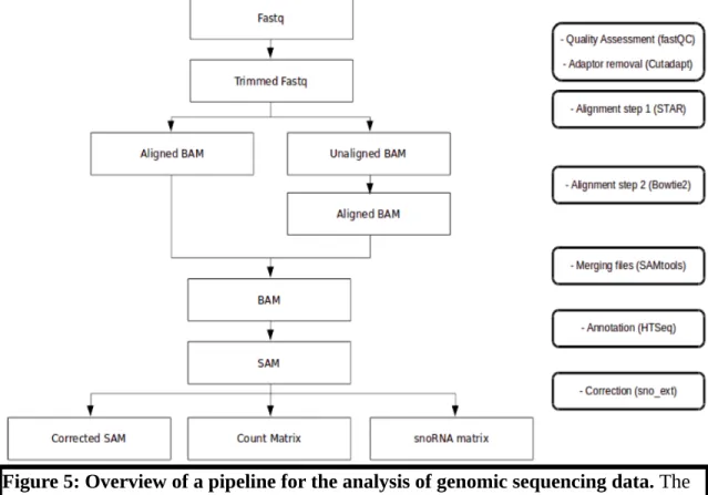
The first step in a computational analysis of genomic sequencing data is to ensure that the sequencing procedure was successful and that the quality of the data is satisfactory. This step of Quality Assessment intakes the raw fastq files that are acquired from the sequencing facilities.

2.2.1 Quality Assessment

The fastq files were run through fastQC (version 0.11.5). The files were inspected for over representation of bases, lower quality bases, and abnormalities in the size of the reads. All files were judged to be of satisfactory quality.

2.2.2 Quality Treatment

Often the small RNAs species were smaller than the read length. As such, part or the entirety of the adaptor sequence would be present within the read. To palliate to the possibility of having an adaptor’s sequence within the 5’ or 3’ of the read, the second step of the bioinformatics pipeline was to remove the adaptor sequences from within the reads.

Figure 5: Overview of a pipeline for the analysis of genomic sequencing data. The data is treated to verify its quality and remove unwanted components (low quality reads and adaptors). The reads are then aligned and annotated to yield various matrices.

The second step was also accompanied with the removal of much lower quality bases from the extremities of the reads. This was done through Cutadapt (version 1.19). Cutadapt is a stand-alone program primarily written in the python programming language with the alignment algorithm being implemented in C. It uses a mismatch threshold and does not require the user to type his own script and functions. As such, Cutadapt is a highly customizable and user-friendly program (Martin, 2011).

The adaptor sequences were given to Cutadapt:

GATCGTCGGACTGTAGAACTCTGAACGTGTAGATCTCGGTGGTCGCCGTATCATT ,

AGATCGGAAGAGCACACGTCTGAACTCCAGTCACATCACGATCTCGTATGCCGT CTTCTGCTTG, TGGAATTCTCGGGTGCCAAGG and

GATCGTCGGACTGTAGAACTCTGAAC

Cutadapt’s parameters were set for the read length threshold to be above 12, with base qualities (phred scores) being above 20, disallowing for indels (insertions or deletions), and allowing for wildcard (unidentified bases) characters. The other parameters remained to their default values which included the error tolerance at 10% of the adaptors’ lengths. The overall command issued to Cutadapt was: cutadapt -a {adaptor_FWD} -A

{adaptor_REV} --minimum-length 13 --no-indels --match-read-wildcards -q 20 -o

{input_reads1}.fastq -p {input_reads2}.fastq {output_reads1}.fastq {output_reads2}.fastq >> {cutadapt_stats}.txt

2.2.3 Alignment

To identify known transcripts from a sequencing dataset, it is, first, common to select an appropriate genome and corresponding annotation. The cell lines being of the human ovarian cancer (SKOV3ip1), the human genome (hg38 version 85), comprising all canonical chromosomes but the Y, was extracted from Ensembl in the fasta format. As for the transcripts and gene annotations, we found out early that various agencies had annotated the human genome which allowed for a certain margin of variation in their respective annotation of transcripts and genes. As such, annotations of the human genome (gtf format) were pooled and repetitions were erased to create a more complete annotation file. The main human genome annotation, hg38 version 85, was extracted from Ensembl (Yates et al., 2016). The Ensembl annotation was supplemented with the genomic transfer RNAs, totalling 628, from the UCSC’s GtRNAdb (Chan & Lowe, 2009). The Ensembl annotation was further modified by adding the snoRNAs, totalling 20, that were found missing from its annotations when crosschecking with RefSeq version 75 (O’Leary et al., 2016). In the goal of identifying variations in the global representation of various small ncRNAs, it was of the utmost importance to find a reliable mechanism by which we could identify ncRNAs. Many algorithms have been implemented in the past and they all achieved various levels of efficacy. However, they have their individual drawbacks such as under representation of smaller species, high run times and high memory allocation requirements. To palliate to these problematic circumstances, multiple alignment programs were used to achieve the most representative species detection possible.

In a first round, the alignment program STAR (version 2.5.1b) was used to capture most of the species. STAR is a stand-alone program written in C++. It used a precompiled index of the target genome which required the input of a gtf file containing the full genomic annotation prior to alignment (Dobin et al., 2013). The aforementioned gtf was fed into STAR (--runMode genomeGenerate, --runThreadN 44, --genomeDir {modified_hg38}.gtf, --genomeFastaFiles {genome}.fasta, --sjdbGTFfile {genome}.gtf, --sjdbOverhang 124) to build a large index (ensembl_star_index}.

The index was later used by STAR to produce the binary alignment map (BAM) files, a binary version of the sam formatted files. The STAR alignment was performed with the following parameters: --runMode alignReads --genomeDir {ensembl_star_index} --readFilesIn {output_reads1}.fastq {output_reads2}.fastq --runThreadN 45 --outReadsUnmapped Fastx --outFilterType BySJout --outStd Log --outSAMunmapped None --outSAMtype BAM SortedByCoordinate --limitGenomeGenerateRAM 250000000000 --limitIObufferSize 4000000000.

Once the first alignment completed, the BAM files contained a few thousand identifiable sequences that had not been mapped properly to snoRNAs. To adjust the BAM files, we used bowtie2 (version 2.2.4) which has the highest sensitivity to smaller (<50nt) species (Langmead & Salzberg, 2012). The first step was to generate an index file for bowtie2 using bowtie2-build and the fasta files containing the chromosomal sequences (Yates et al., 2016). The BAM files containing the unmapped reads were sorted and changed back to fastq format using bam2fastx. The resulting sorted fastq file was fed into bowtie2 with the parameters for local alignment of a minimal length of 13 bps using 48 processes and the human gtf file previously mentioned (bowtie2 --local -p 48 -q -x {bowtie2_index} -1 {unmapped1}.fastq -2 {unmapped2}.fastq -I 13 -S {htseq_annotated}.sam). Bowtie2 outputted a SAM file which was merged with the output from the mapping step with STAR using SAMtools (version 1.3).

2.2.4 Read Annotation

Once the second alignment step was completed and the reads were mapped to genomic intervals, these intervals were associated to genes and transcripts to estimate gene counts. This estimation can be obtained from a number of ways. One of the most common is to add a field in the mapping file indicating the gene / transcript found at the specified genomic interval. This process can become more involved when specific splicing variants of exons have to be measured. However, measuring exons’ expression falls outside of this experiment’s scope of interest. The program used in the annotation process had to be simple to use, to modify and it had to be well documented.