From planar graphs to higher dimension

(1)

HAL Id: tel-02931761

https://tel.archives-ouvertes.fr/tel-02931761

Submitted on 7 Sep 2020

HAL is a multi-disciplinary open access

archive for the deposit and dissemination of

sci-entific research documents, whether they are

pub-lished or not. The documents may come from

L’archive ouverte pluridisciplinaire HAL, est

destinée au dépôt et à la diffusion de documents

scientifiques de niveau recherche, publiés ou non,

émanant des établissements d’enseignement et de

From planar graphs to higher dimension

Lucas Isenmann

To cite this version:

Lucas Isenmann. From planar graphs to higher dimension. Discrete Mathematics [cs.DM]. Université

Montpellier, 2019. English. �NNT : 2019MONTS142�. �tel-02931761�

(2)

Devant le jury composé de

Jean CARDINAL, Professeur, Université Libre de Bruxelles

Nicolas BONICHON, Maitre de conférences, Université de Bordeaux William PUECH, Professeur des universités, Université de de Montpellier Nicolas TROTIGNON, Directeur de recherche, ENS de Lyon

Rapporteur Examinateur Examinateur Examinateur

Présentée par Lucas Isenmann

Décembre 2019

Sous la direction de Daniel GONÇALVES

Des graphes planaires vers des dimensions supérieures

THÈSE POUR OBTENIR LE GRADE DE DOCTEUR

DE L’UNIVERSITÉ DE MONTPELLIER

En informatique

École doctorale I2S

(3)

Introduction

Graphs. Graph theory has been invented in order to study networks. In this theory we focus on the connections between some kind of objects and not directly on the objects. Applications arise in a large panel of domains. But maybe one that is massively used directly every day, is when you look for an itinerary on an online map. The user asks to the software what is the best path to go from point A to point B in the transport network. It may seem an easy problem for the user of the software, but behind it, there are years of research in graph theory for making it possible and efficient. In this network, the objects are locations in the world and we consider that two locations are connected if there is a road between them. Moreover, asking the best path in this network is not the only question. You can also ask “what is the fastest way to visit all the towns of a region?”. In addition to the previous questions, the transport networks have raised numerous problems in graph theory which have become very important with the development of computer science.

But transport networks are not the only networks that can be modeled with graphs. An application which has gained a lot of interest recently, thanks to the development of the internet and to the storage capacity of computers is the study of social networks: the objects here are the people in the world, and we consider that two persons are connected if they know each other (in some way). In this kind of network, you can try to detect communities or to know who are the central persons. Applications are numerous: you can study for example the spreading of a rumor.

We finally give another application in biology where we can study the spread-ing of a disease. For instance, you can consider a region of the world and a biologic network where the objects are some points in the region where some species exists. We consider that two points are connected if there is a movement of a part of the population from one point to the other point. In that case, we say that the network is oriented because the connections are not symmetric as a movement from a point A to a point B does not imply a movement from B to A. Furthermore, in this network the connections are said to be weighted by the proportion of moving.

In the terminology of graph theory, networks are called graphs, objects are called vertices and connections are called edges. As we have seen, every network is different and can be modeled by different graph models (for example oriented graphs, or weighted graphs). Among these different types of graphs, we focus in this thesis on one particular type: planar graphs.

(6)

Planar graphs. A graph is planar if it is possible to draw it in the plane such that two edges can only intersect at endpoints. A very important example is the road network if there is no road passing over another one (with the help of a bridge or a tunnel). This is for instance the case in the problem of the seven bridges of K¨onigsberg solved by Euler in 1736 and which may be considered as the first use of graph theory.

Figure 1: The seven bridges of the K¨onigsberg problem.

Another fundamental problem is the problem of coloring a planar graph. Consider a cartography of the french metropolitan departments map where you want to color the departments such that no two adjacent departments have the same color. How much colors will you have to use? The solution is four as you can see on Figure 2 and this result is known since Appel and Haken proved it in 1976 [26]. Planar graphs are also related to the notion of meshes used in computer-aided design in order to draw 3D model of objects [81].

In addition to their practical applications, planar graphs are mathematically important because they form a big class of graphs which has a lot of good properties and a lot of useful tools which make them a good starting point to tackle a new problem. For instance, the celebrated graph minor theorem from Robertson and Seymour uses planar graphs in the beginning of the proof [97].

Due to the importance of planar graphs in practical and in theoretical as-pects, tools have been developed for this class of graphs as we will see.

Dushnik-Miller dimension. Among the useful properties and tools that planar graphs have, there is the Dushnik-Miller dimension whose definition re-quires the notion of posets. A poset is an abstract set of elements where the elements are arbitrarily ordered by assuming that some elements are greater, lesser or incomparable than some other elements. While in a poset, two elements are not necessarily comparable, a linear order is a poset such that every pair of elements are comparable. The Dushnik-Miller dimension, also known as the order dimension, of a poset is an integer which measures the default of linearity of the poset in some sense (as a linear poset has Dushnik-Miller dimension 1 and

(7)

Figure 2: A four coloration of the departments the metropolitan France map.

a poset which is not linear has Dushnik-Miller dimension strictly bigger than 1).

Dushnik-Miller dimension can be applied to graphs as follows. We can define the incidence poset of a graph which captures the fact that a vertex is incident or not to an edge. The Dushnik-Miller dimension of a graph G can be defined as the Dushnik-Miller dimension of the incidence poset of G. A theorem of Schnyder [100] states that a graph is planar if and only if Dushnik-Miller dimension of this graph is at most 3. As a consequence of this theorem, the notion of planarity can be seen as a combinatorial property while it is defined as a topological one. According to the previous theorem of Schnyder, planar graphs correspond to graphs whose incidence poset has Dushnik-Miller dimension at most 3. The Dushnik-Miller dimension of a graph could be therefore considered as a measure of the geometrical complexity of this graph. A natural question, as raised by Trotter in [104], is to find a generalization of the theorem of Schnyder to higher dimensions. This question was tackled by Ossona de Mendez [92] and Felsner and Kappes, who found partial results in this direction [67]. In this thesis we investigate if it is possible to answer this question with the help of two different geometric classes of graphs. The first one is a particular class of intersection graphs.

Intersection graphs. Intersection graphs are defined in the following way. Consider some geometric objects in a geometric space and consider the inter-section graph of these objects where a vertex corresponds to an object and an edge corresponds to an intersection between two objects. This kind of graphs have been widely studied with variations on the considered objects and on the way that these objects intersect. When the objects possibly have an “interior

(8)

intersection” with other objects, we use the term X-intersection graph, where X is a description of the allowed geometrical objects. When the objects have no interior intersection with other objects, then the term X-contact graph is pre-ferred. We now give some examples of intersection graphs and of some contact graphs which have been proved to be practically important.

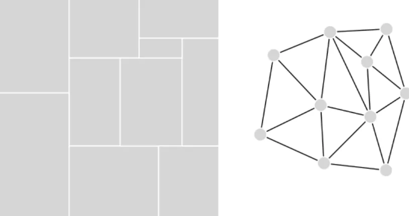
Examples of intersection graphs can be obtained by considering unit disks in the plane. We can form the intersection graph of these disks (see Figure 3). We say that a graph is a unit disk graph if it is the intersection graph of unit disks in the plane. This kind of graphs are used in communication networks where a disk corresponds to the range of an antenna [77].

Figure 3: An example of a unit disk arrangement and its associated intersection graph.

Examples of contact graphs can be obtained by considering circles in the plane such that no two disks have an interior intersection. Such an arrangement of circles is called a circle packing (see Figure 4). As there are no interior intersection, we can consider the contact graph of this circle packing. The celebrated circle packing theorem by Koebe [16] states that a graph is planar if and only if it is the contact graph of a circle packing. This theorem was recently used to re-prove the planar separator theorem [90] and to find drawings of planar graphs with bounded angular resolution [86].

The second type of geometric graphs class used in the goal of answering the previous question on the generalization of the Theorem of Schnyder is the class of TD-Delaunay graphs.

TD-Delaunay graphs. TD-Delaunay graphs are a variant of the well-known class of Delaunay graphs. Given points in the plane, the Delaunay graph of this set of points is defined as follows: two points are considered to be adjacent if there exists a disk containing these two points but no other point in its interior (see Figure 5a for an example). Delaunay graphs have plenty of geometrical properties which made them of particular interest in algorithms generating tri-angular meshes [42]. The class of TD-Delaunay graphs is defined in a similar way by replacing disks by equilateral triangles in the previous definition (see Figure 5b for an example). They were introduced by Chew and Drysdale [37] and are used by Chew [43] in the problem of finding sparse spanners.

(9)

Figure 4: An example of a circle packing and its associated contact graph.

(a) An example of a Delaunay graph where the construction cir-cles are in grey.

(b) An example of a TD-Delaunay graph where the construction tri-angles are in grey.

Figure 5: Examples of Delaunay and TD-Delaunay graphs.

Organization of the thesis. In the first chapter, we investigate a generaliza-tion of Schnyder’s theorem for higher Dushnik-Miller dimension. Three results are proved in this chapter. The first result is that TD-Delaunay complexes do not characterize Dushnik-Miller dimension (contradicting a conjecture). The second result is a generalization of some topological properties of some simplicial complexes linked to the Dushnik-Miller dimension. The third result investigates a new class of contact graphs, called stair packings, which are contact graphs of shapes similar to “stairs” when drawn in the plane, and studies the link between these graphs and the Dushnik-Miller dimension.

In the last two chapters, results on planar graphs are proved. We hope that these results could be generalized in some sense as it the case of the results proven in the first chapter.

The second chapter deals with x-intersection graphs and x-contact graphs, which are intersection graphs of shapes similar to “x” drawn in the plane. The proven results in this chapter are characterizations of these graphs in terms of planarity and could be generalized to higher dimensions.

(10)

In the third chapter we introduce the new notion of M¨obius stanchion sys-tems defined on planar graphs. This notion is connected to the problem of finding a drawing of a planar graph on any closed surface, like a sphere or a “donut”, such that there is only one face.

(11)

Introduction

Graphes. La théorie des graphes a été développée pour étudier les nombreux réseaux utilisés dans le monde scientifique. Dans cette théorie on ne s’intéresse pas directement à des objets mais au système que forment les connexions entre ces différents objets. On peut trouver des applications dans de nombreux do-maines. Parmi ces applications, celle qui consiste à chercher son chemin sur une carte en ligne est massivement utilisée tous les jours. L’utilisateur demande au logiciel quel est le plus court chemin entre un point A et un point B du réseau de transport. Du point de vue de l’utilisateur ce problème peut paraˆıtre facile mais des années de recherches en théorie des graphes ont été nécessaires pour résoudre ce problème en un temps concis. Dans ce réseau particulier, les objets sont par exemple des villes et on considère que deux villes sont connectées entre elles s’il y a une route directe qui relie l’une à l’autre. Résoudre la question du plus court chemin n’est pas l’unique question intéressante que l’on peut se poser sur le réseau de transport. On peut aussi chercher le chemin le plus rapide pour visiter toutes les villes d’une région. En plus de ces questions, le réseau de transport a soulevé de nombreux problèmes de théorie des graphes qui sont devenus de plus en plus important avec l’avènement de l’informatique.

Mais les réseaux de transports ne sont pas les seuls réseaux qui peuvent être modélisés avec des graphes. L’étude des graphes sociaux est un nouveau domaine d’application qui est apparu récemment grâce au développement de l’internet et à l’augmentation des capacités de stockage des ordinateurs. Dans ce type de graphes les objets sont les êtres humains et on considère que deux personnes sont reliées entre elles si elles se connaissent en un certain sens que le modèle doit définir. Dans ce type de réseau, on peut essayer par exemple de chercher à discerner des communautés ou à trouver les personnes centrales. Les applications sont nombreuses : on peut par exemple étudier la diffusion de rumeurs.

En biologie aussi on peut utiliser les graphes. C’est par exemple le cas quand on s’intéresse au développement d’une maladie virale dans la population humaine. Un second exemple consiste à considérer une région du monde où vit une espèce animale. On peut supposer que deux localisations de cette région sont connectées dans ce modèle s’il y a un mouvement d’une partie de la population entre ces deux localisations. Dans ce cas, on dit que le réseau est orienté car les connexions ne sont pas symétriques : le déplacement d’une partie de la population se fait d’un point A vers un point B et n’implique pas un déplacement

(12)

dans l’autre sens. De plus dans ce réseau les connexions peuvent être pondérés par l’importance du déplacement.

Dans la terminologie de la théorie des graphes, les réseaux sont appelés graphes, les objets sommets et les connexions arêtes. Comme on l’a vu, chaque réseau est différent et peut être modélisé par différents modèles de graphes (comme les graphes orientés ou pondérés). Parmi ces types de graphes, on s’intéresse particulièrement dans cette thèse à un type particulier : les graphes planaires.

Les graphes planaires. Un graphe est dit planaire si on peut le dessiner dans le plan de sorte que les arêtes ne se croisent qu’à leurs extrémités. Un exemple de graphe planaire très important est le réseau de transport, si l’on suppose qu’il n’y ait pas de route qui passe au-dessus d’une autre par l’intermédiaire d’un pont ou d’un tunnel. C’est par exemple le cas dans le problème des sept ponts de Königsberg qui a été résolu par Euler en 1736 et qui peut être considéré comme la première utilisation de la théorie des graphes.

Figure 6: Le probl`eme des sept ponts de K¨onigsberg.

Un autre problème fondamental est le problème de coloration d’un graphe planaire. Considérons une carte de la France métropolitaine où l’on veut colorier les départements de sorte que deux départements adjacents n’aient pas la même couleur. Combien de couleurs faut-il utiliser ? Appel et Haken [26] ont résolu ce problème en 1976 et ont démontré que le nombre de couleurs nécessaires est quatre comme le montre la Figure 7. Les graphes planaires sont aussi reliés à la notion de maillage qui est utilisée en dessin assisté par ordinateur pour dessiner des modèles 3D d’objets [81].

En plus de leurs applications pratiques, les graphes planaires ont un intérêt mathématique car ils forment une vaste classe de graphes possédant de nom-breuses propriétés et des outils dédiés qui en font un bon point de départ pour s’attaquer à un problème. C’est par exemple le cas du célèbre théorème sur les mineurs de graphes de Robertson et Seymour qui utilise les graphes planaires au début de sa démonstration [97].

(13)

Figure 7: Une coloration de la carte des d´epartements m´etropolitains fran¸cais avec quatre couleurs.

Du fait de l’importance des graphes planaires en pratique et en théorie, des outils ont été développés pour cette classe de graphes comme on va le voir. La dimension de Dushnik-Miller. Parmi les propriétés et outils utiles que possèdent les graphes planaires, il y a la dimension de Dushnik-Miller dont la définition nécessite la notion d’ordre. Un ordre est la donnée d’un ensemble abstrait d’éléments où ces éléments sont arbitrairement classés en supposant que certains sont plus grands ou plus petits que d’autres; deux éléments peu-vent aussi être supposés incomparables. Alors que dans un ordre en général deux éléments ne sont pas forcément comparables, un ordre total (ou ordre linéaire) est un ordre où chaque paire d’éléments est comparable. La dimension de Dushnik-Miller, aussi connue sous le nom de dimension d’ordre, est un entier qui mesure le défaut de linéarité d’un ordre en un certain sens : un ordre sera de dimension Dushnik-Miller 1 si et seulement si cet ordre est linéaire.

La dimension de Dushnik-Miller peut être appliquée aux graphes en con-sidérant son ordre d’incidence. Cet ordre particulier capture le fait qu’un som-met soit incident ou non à une arête. La dimension de Dushnik-Miller d’un graphe est ainsi définie comme la dimension de Dushnik-Miller de son ordre d’incidence. Le théorème de Schnyder [100] assure qu’un graphe est planaire si et seulement s’il est de dimension de Dushnik-Miller au plus 3. Une conséquence de ce théorème est que la notion topologique de planarité peut être vue comme une propriété combinatoire du graphe.

Comme le montre le théorème précédent de Schnyder, la dimension de Dushnik-Miller pourrait mesurer la complexité géométrique d’un graphe. Une question naturelle soulevée par Trotter dans [104] consiste à trouver une généralisation

(14)

du théorème de Schnyder pour des dimensions supérieures. Cette question a été abordée par Ossona de Mendez [92] et Felsner et Kappes [67] qui ont trouvé des résultats partiels dans ce sens. Dans cette thèse on étudie la possibilité de répondre à cette question à l’aide de deux classes de graphes géométriques. La première est un cas particulier de graphes d’intersection.

Les graphes d’intersection. Les graphes d’intersection sont définis de la manière suivante. En considérant des objets géométriques dans un espace géométrique particulier on peut définir le graphe d’intersection de ces objets par un graphe où un sommet correspond à un objet et une arête correspond à une intersection entre deux objets. Ce type de graphes a été largement étudié tout comme les variations qui peuvent être apportées aux objets considérés ou `

a la manière dont ces objets s’intersectent. Quand les objets ont possiblement une intersection intérieure avec d’autres objets, on préférera utiliser le terme de graphe d’intersection de X où X est une description des objets géométriques autorisés. Quand les objets n’ont pas d’intersection intérieure, on préférera le terme de graphe de contact de X. On donne maintenant des exemples de graphes d’intersection et de graphes de contact qui sont importants en pratique.

Des exemples de graphes d’intersection peuvent être obtenus en considérant des disques unités dans le plan. A partir de ces disques on peut former le` graphe d’intersection (voir Figure 8). On dit qu’un graphe est un graphe de disques unitéss’il s’agit du graphe d’intersection de disques unités dans le plan. Ce type de graphes est par exemple utilisé dans les réseaux de communications où les disques représentent le rayon d’action d’une antenne [77].

Figure 8: Un exemple d’arrangement de disques unit´es et son graphe d’intersection associ´e.

En considérant des disques dans le plan qui ne s’intersectent pas en un point intérieur, on obtient ce que l’on appelle un empilement de disques (voir Figure 9). Comme il n’y a pas d’intersection intérieure, on peut considérer le graphe de contact de cet arrangement. Le célèbre thérorème d’empilement de disques de Koebe [16] assure qu’un graphe est planaire si et seulement si c’est le graphe de contact d’un empilement de disques. Ce théorème a été récemment utilisé pour reprouver le théorème du séparateur planaire [90] et pour trouver des plongements de graphes planaires avec un angle de résolution borné [86].

(15)

Figure 9: Un exemple d’empilement de disques et son graphe de contact associ´e.

Le second type de graphes géométriques utilisé pour répondre à la question du paragraphe précédent sur la généralisation du théorème de Schnyder est la classe des graphes de TD-Delaunay.

Les graphes de TD-Delaunay. Les graphes de TD-Delaunay sont des vari-antes des graphes de Delaunay. Étant donné des points dans le plan, le graphe de Delaunay de cet ensemble de points est défini comme suit : deux points sont considérés comme adjacents s’il existe un disque contenant ces deux points mais aucun autre point à l’intérieur (voir l’exemple sur la Figure 10a). Les graphes de Delaunay ont de nombreuses propriétés géométriques qui confèrent à ces graphes un intérêt particulier dans les algorithmes générant des maillages triangulaires [42]. La classe des graphes de TD-Delaunay est définie de manière similaire en rempla¸cant dans la définition précédente les disques par des trian-gles équilatéraux (voir l’exemple sur la Figure 10b). Ils ont été définis par Chew et Drysdale [37] et ont été utilisés par Chew [43] dans le problème consistant à chercher des spanners creux.

(a) Un exemple de graphe de De-launay o`u les disques de construc-tion sont en gris.

(b) Un exemple de graphe de TD-Delaunay o`u les triangles de con-struction sont en gris.

(16)

Organisation de la thèse. Dans le premier chapitre, on s’intéresse à la généralisation du théorème de Schnyder aux dimensions supérieures. On démontre dans ce chapitre trois résultats dans ce sens. Le premier assure que les com-plexes de TD-Delaunay ne caractérisent pas la dimension de Dushnik-Miller (ce qui contredit une conjecture de Mary [87] et de Evans et al. [48]). Le deuxième résultat généralise des propriétés topologiques de certains complexes simpliciaux connectés à la dimension de Dushnik-Miller. Le troisième résultat concerne une nouvelle classe de graphes de contact, appelé graphes de contacts d’escaliers, où les contacts se font entre des formes ressemblant à des escaliers dans le plan. Ce dernier résultat fait le lien entre de tels graphes et la dimension de Dushnik-Miller.

Dans les deux derniers chapitres, on d´emontre des r´esultats sur les graphes planaires.

Le deuxième chapitre concerne plus spécifiquement les graphes d’intersection de x et les graphes de contact de x qui sont des graphes d’intersection de formes ressemblant à des “x” dessinés dans le plan. On montre dans ce chapitre que l’on peut représenter certains types de graphes planaires comme des graphes de contacts ou d’intersection de x. Ces résultats pourraient être généralisés en dimension supérieure.

Dans le troisième chapitre on introduit la notion de systèmes de Möbius stanchions qui est définie sur les graphes planaires. Cette notion est connectée au problème consistant à trouver un plongement d’un graphe planaire sur une surface fermée, comme une sphère ou un tore, de sorte qu’il n’y ait qu’une face.

(17)

General definitions

Graphs and planarity

Given a finite set V and a subset E of the pairs of V , we define the graph G = (V, E). Elements of V are called vertices and elements of E are called edges. An edge e is incident to a vertex v if v_{∈ e. Two edges e and e}0 _{are said}

to be adjacent if there exists a vertex v such that v is incident to both of them. Two vertices are said to be adjacent if E contains the pair consisting in this pair of two vertices. The degree of a vertex is the number of edges incident to this vertex. Given F a subset of the vertices of a graph G, the graph G\ F obtained after the removal of the vertices of F consists in the graph whose vertex set is V \ F and whose edge set is the edges of G not incident to some vertices of F . A path is sequence e1, . . . , ek of edges such that ei is adjacent to ei+1 for every

i∈ [[1, d − 1]]. We say that a graph G is connected if for every pair of vertices x and y, there exists a path e1, . . . , ek of G such that e1 is incident to x and ek

is incident to y. Otherwise we say that the graph is disconnected. A graph is k-connected if and only if any removal of k_{− 1 vertices does not disconnect the} graph. A graph is said to be a tree if it is connected and if_{|V | = |E| + 1. Given} a graph G, a spanning tree of G is a subgraph T of G such that T is a tree and such that the vertices of T and G are the same. An orientation of a graph consists in giving a direction to each edge. Given a vertex v and an incident edge e, we say that e is in-going (resp. out-going) if e goes to v (resp. come from v).

Planarity. A graph is said to be planar if it is possible to draw it in the plane such that edges only intersect at endpoints. A plane graph is a graph given with an embedding of the graph in the plane. A face of a plane graph is a connected component of R2\G. The infinite face is called the outer face, while the other faces are called inner faces. The dual of a plane graph G, noted G∗_{, is a graph}

whose vertex set consisting in the faces of G and where two faces are considered to be connected if there exists an edge of G which separates these two faces. A near-triangulation is a plane graph such that every inner face is triangular. A triangulationis a near-triangulation such that the outer face is triangular. In a plane graph G, a chord is an edge not bounding the outer face but that links two vertices of the outer face. A separating triangle of G is a cycle of length three such that both regions delimited by this cycle (the inner and the outer region) contain some vertices.

We recall the following theorem:

Theorem 1(folklore). A triangulation is 4-connected if and only if it contains no separating triangle.

Intersection graphs and contact graphs

The representation of graphs by contact or intersection of predefined shapes in the plane is a broad subject of research since the work of Koebe on the

(18)

representation of planar graphs by contacts of circles [16]. In particular, the class of planar graphs has been widely studied in this context.

Definition 2. Given a shape1 X, an X-intersection representation is a col-lection ofX-shaped geometrical objects in the plane. The X-intersection graph described by such a representation has one vertex per geometrical object, and two vertices are adjacent if and only if the corresponding objects intersect. Definition 3. In the case where the shape X defines objects that are home-omorphic to a segment (resp. to a disc), an X-contact representation is an X-intersection representation such that if an intersection occurs between two objects, then it occurs at a single point that is the endpoint of one of them (resp. it occurs on their boundary). We say that a graphG is an X-contact graph if it is theX-intersection graph of an X-contact representation.

The case of shapes homeomorphic to discs has been widely studied; see for example the literature for triangles [12, 10], homothetic triangles [9, 7], axis parallel rectangles [103], squares [5, 6], hexagons [11], convex bodies [8], or axis aligned polygons [4].

1_{We do not provide a formal definition of shape, but a shape characterizes a family of}

(19)

Chapter 1

Dushnik-Miller dimension

of some geometric

complexes

In this chapter we focus on combinatorial properties of two types of geometri-cally defined simplicial complexes through the lens of Dushnik-Miller dimension. The first one is the class of TD-Delaunay complexes which is a generalization of the class of TD-Delaunay graphs in the plane which is itself a variation of the well-known class of Delaunay graphs. The second one concerns stair packing contact complexes. This new kind of contact complexes is directly connected to the Dushnik-Miller dimension.

1.1 Introduction

1.1.1 Basic notions

We now recall the following basic notions of order theory. Given a set V , a poset (V,_{≤) is a binary relation ≤ on V satisfying the following properties for every} a, b, c_{∈ V :}

• a ≤ a (reflexivity);

• if a ≤ b and b ≤ c, then a ≤ c (transitivity); • if a ≤ b and b ≤ a, then a = b (antisymmetry).

A linear order on a set V , is a poset on V such that for every pair (a, b) of elements of V , a ≤ b or b ≤ a. Given a poset (V, ≤), a linear extension is a linear order≤0_{on V such that for every pair (a, b)}_{∈ V}2_{, a}_{≤ b ⇒ a ≤}0 _{b. When}

the set V is finite, there always exists a linear extension of a poset on V . The digraph of the poset (V,≤) is the digraph whose vertex set is V and where there

(20)

is an arc from x to y when x_{≤ y for every pair (x, y) of elements of V . The} transitive reduction of a digraph D is a subgraph D0 with the fewest arcs such that for every pair (x, y) of elements of V , there exists a directed path from x to y in D if and only if there exists a directed path from x to y in D0. Note that the transitive reduction of a digraph is unique. The Hasse diagram of a poset is the transitive reduction of the digraph of the poset. Given a linear order (V,≤) and a finite subset F of V , we define max≤(F ) as the maximum of the set F

according to the linear order_≤.

We will also use the notion of abstract simplicial complexes which generalizes the notion of graphs. An abstract simplicial complex ∆ with vertex set V is a set of subsets of V which is closed by inclusion (i.e. _{∀Y ∈ ∆, X ⊆ Y ⇒ X ∈ ∆).} An element of ∆ is called a face. A maximal element of ∆ according to the inclusion order is called a facet.

B

A C

D E

F G

Figure 1.1: An abstract simplicial complex whose facets are

{A, B, C, D},{C, D, E},{C, F }, {E, F } and {F, G}.

The dimension of a face F is defined as_{|F | − 1. A simplicial complex is said} to be pure if all its facets have the same dimension.

Given a simplicial complex ∆, we define the inclusion poset of ∆ as the poset (∆,_{≤) defined on the faces of ∆ where X ≤ Y for any pair (X, Y ) ∈ ∆}2 _such

that X_{⊆ Y .}

The following lemma will be used to study the Dushnik-Miller dimension. Lemma 4. Let _≤0 be a linear order on a finite set V . The binary relation ≤ defined on Subsets(V ) by

F _{≤ G ⇐⇒}

(

F ⊆ G, or

F _{6⊆ G and G 6⊆ F and max}_≤0(F \ G) <0 max_≤0(G\ F )

is a linear extension of the inclusion poset on Subsets(V ).

Proof. The relation _{≤ is clearly reflexive. Let us show that it is also} antisym-metric. Let F and G be two faces of ∆ such that F _{≤ G and G ≤ F . Suppose by} contradiction that F _{6= G. Suppose first that F ⊆ G. As G ≤ F , then G ⊆ F or} max≤0(G\F ) <0 max_≤0(F\G). The latter is impossible as F \G = ∅, and the

for-mer implies that F = G, a contradiction. Thus F _{6⊆ G. Similarly, we have that} G_{6⊆ F . As F ≤ G and G ≤ F , we deduce that max}≤0(F \ G) <0max_≤0(G\ F )

(21)

and that max≤0(G\ F ) <0 max_≤0(F\ G) which is a contradiction. We conclude

that F = G and that≤ is antisymmetric.

Let us show that the relation≤ is transitive. Let F , G and H be three faces of ∆ such that F ≤ G ≤ H. Suppose first that F ⊆ G and G ⊆ H. Then F⊆ H and F ≤ H.

Suppose now that F 6⊆ G and G ⊆ H. As F ≤ G, we deduce that G 6⊆ F . If F ⊆ H, then F ≤ H. Otherwise F 6⊆ H. If H ⊆ F , then we have G ⊆ F , as G_{⊆ H, which is a contradiction. Thus H 6⊆ F . As G ⊆ H, we have that} F_{\ H ⊆ F \ G and G \ F ⊆ H \ F . Thus} max ≤0 (F \ H) ≤ 0_max ≤0 (F \ G) < 0_max ≤0 (G\ F ) ≤ 0 _max ≤0 (H\ F )

We conclude that F _{≤ H. The case where F ⊆ G and G 6⊆ H is similar.} It remains to study the case where F _{6⊆ G and G 6⊆ H. If F ⊆ H, then} F _{≤ H. Otherwise F 6⊆ H. Suppose by contradiction that we have not the} inequality max≤0(F \ H) <0max_≤0(H\ F ). We define max_≤0(∅) as an element

such that max≤0(∅) <0min_≤0(V ). We define the following elements:

                   a = max≤0(F \ (GS H)) b = max≤0((FT G) \ H) c = max≤0(G\ (FS H)) d = max≤0((GT H) \ F ) e = max≤0(H\ (FS G)) f = max≤0((HT F ) \ G)

Because of the different hypotheses we have      max(a, f ) <0max(c, d) max(b, c) <0_{max(f, e)} max(d, e) <0_{max(a, b)}

Suppose that c_≤0 _{d. In this case, a <}0 _{d and f <}0 _{d. As d <}0 _{max(a, b), then}

d <0 _{b. As b <}0 _{max(f, e) and f <}0 _{d <}0 _{b, then b <}0 _{e. As e <}0 _{max(a, b) and}

a <0 _{d <}0 _{b, then e <}0_{b, a contradiction. The case where d}_≤0_{c is symmetrical.}

We conclude that the binary relation≤ on Subsets(V ) is reflexive, antisym-metric and transitive. Therefore ≤ is an order. As ≤0 _{is a linear order, we}

deduce that≤ is also a linear order. Furthermore if F ⊆ G, then F ≤ G. We conclude that≤ is a linear extension of the inclusion poset on Subsets(V ).

1.1.2 Delaunay graphs and their variants

Original Delaunay graphs are defined as follows.

Definition 5. Given a set of points_{P in R}2 such that no quadruplet of _{P lies} on one circle, the Delaunay graph D(_{P) of P is defined as the graph with vertex}

(22)

set_{P and where the vertices are connected as follows. Two points are connected} if and only if there exists a closed disk containing these two points but no other point in the interior of this disk.

An example of a Delaunay graph is given in Figure 1.2. An interesting property of these graphs is the following:

Theorem 6. Given a set of points_{P in R}2 such that no quadruplet of_{P lies} on one circle, the graphD(_{P) is a near-triangulation.}

Figure 1.2: An example of a Delaunay graph. Construction circles are in grey. The class of Delaunay graphs can be generalized with the use of convex distance functions.

Definition 7. Given a compact convex subset S of Rd and a point c in the interior ofS, we define the convex distance function f , also called Minkowski distance function, between two points p and q as the minimal scaling factor f (p, q) = λ such that after rescaling S by λ and translating it so as to center it onp, then it contains also q.

The convex distance function associated to the unit disk in Rd where c is the center of this disk is the Euclidean distance. Any distance associated to a norm in Rd is a convex distance function by taking S as the unit disk in Rd according to this norm and c as the center of this disk. The reciprocal of the previous statement is false, as convex distance functions do not satisfy the symmetry property of distances in general. By taking S an equilateral triangle in the plane and c the center of this triangle, we get the convex distance function called triangular distance which is abbreviated TD.

Definition 8. Given a set of points_{P in R}2 and a convex distance functionf , for a pointx_{∈ P, we define its f-Voronoi cell as the set of points y of the plane}

(23)

such thatx is among the nearest points of P , according to the convex distance function f , to y, i.e. the set of points {y : f(x, y) ≤ f(x0_{, y)} _∀x0 _{∈ P}. We}

define thef -Delaunay graph of a point setP as the graph with vertex set P such that two points are connected if and only if theirf -Voronoi cells intersect.

Delaunay graphs are particular cases of f -Delaunay graph by taking f as the Euclidean distance. The TD-Delaunay class of graphs is therefore defined as the class of f -Delaunay graphs where f is the triangular distance. Note that TD-Delaunay graphs also admit an alternative definition similar to Definition 5: Definition 9. Given a set _{P of points of R}2 in general position, let the TD-Delaunay graph of_{P, denoted by TDD(P), be the graph with vertex set P defined} as follows. A subset F _{⊆ P is a face of TDD(P) if and only if there exists an} equilateral triangleT with one horizontal edge at the top such that T _{∩ P = F} and such that no point of_{P is in the interior of T .}

Figure 1.3: An example of a TD-Delaunay graph. Construction triangles are in grey.

Bonichon et al. [31] observed the following property of TD-Delaunay graphs. Theorem 10(Bonichon et al. [31]). A graph G is planar if and only if G is a subgraph of a TD-Delaunay graph.

TD-Delaunay graphs can be generalized to higher dimensions by taking the triangular distance in Rdaccording to a regular d-simplex. As a graph is planar if and only if G is of Dushnik-Miller dimension, whose definition will be given latter, at most 3, there is maybe a link between the notions of Dushnik-Miller dimension and TD-Delaunay complexes. In [87] and [48] it was independently asked whether Dushnik-Miller dimension at most d complexes are exactly the subcomplexes of TD-Delaunay complexes of Rd−1.

Spanners

Spanners were introduced by Chew [41] and are used in motion planning and network design. This notion motivated the introduction of the previous variants of Delaunay graphs.

(24)

Definition 11. Given points in the plane, a plane spanner is a subgraph of the complete graph on these points which is planar when joining adjacent points with segments.

The stretch of a plane spanner is the maximum ratio of the distance in the graph between two vertices where edges are weighted accordingly to their length and the Euclidean distance between these two points.

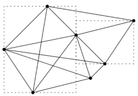
0 2

3

4 1

Figure 1.4: An example of a plane spanner. The stretch of this spanner is 4 as the distance between vertices 0 and 4 is 4 times larger than the Euclidean distance between these two vertices.

Given points in the plane, a natural question which has attracted a lot of attention is to find a plane spanner which minimizes the stretch. We define the stretch of a class of spanners as the maximum stretch among them. Chew [41] found the first class of plane spanners with finite stretch which consists in the class of L1-Delaunay graphs. Chew [41] also conjectured that the class of L2

-Delaunay graphs (classical -Delaunay graphs) has a finite stretch. This question initiated a series of papers about this topic which droped the upper bound from 5.08 to 1.998 [32, 45, 106]. The stretch of the class of TD-Delaunay graphs is 2 according to [43].

In higher dimensions, finding a class of graphs with finite stretch is an active domain of research. We conjecture that the stretch of the class of TD-Delaunay graphs in Rd is d. A lower bound can be easily obtained by putting a point in each “corner” of a regular d-simplex in Rd.

1.1.3 Dushnik-Miller dimension and representations

The notion of Dushnik-Miller dimension of a poset has been introduced by Dushnik and Miller [46]. It is also known as the order dimension of a poset. See [104] for a comprehensive study of this topic.

Definition 12. TheDushnik-Miller dimension of a poset (V,_{≤) is the minimum} number d such that (V,≤) is the intersection of d linear extensions of (V, ≤). This means that there exists d linear extensions (V,≤1), . . . , (V,≤d) of (V,≤)

such that for everyx, y∈ V , x ≤ y if and only if x ≤iy for every i∈ [[1, d]]. In

particular ifx and y are incomparable with respect to≤, then there exists i and j such that x≤iy and y≤jx.

(25)

b1 b2 b3

a1 a2 a3

a1<1a2<1b3<1a3<1b1<1b2

a2<2a3<2b1<2a1<2b2<2b3

a1<3a3<3b2<3a2<3b1<3b3

Figure 1.5: A poset _{≤ defined by its Hasse diagram and 3 linear extensions} ≤1,≤2 and≤3of≤ showing that ≤ is of Dushnik-Miller dimension at most 3.

The notion of Dushnik-Miller dimension can be applied to a simplicial com-plex as follows.

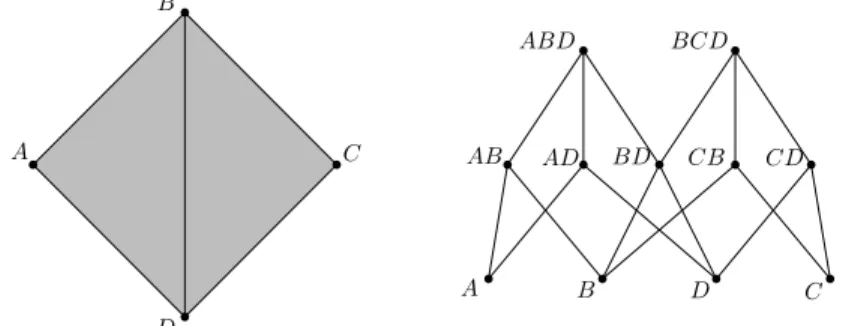
Definition 13. Let ∆ be a simplicial complex. We define the Dushnik-Miller dimension of ∆, denoted dimDM(∆), as the Dushnik-Miller dimension of the

inclusion poset of∆. A B C D ABD BCD BD AB AD CD A B D C CB

Figure 1.6: A simplicial complex with facets_{{A, B, D} and {B, C, D}, and its} inclusion poset.

Low dimensions are well known. We have dimDM(∆) = 1 if and only

if ∆ is a union of single vertices. We have dimDM(∆) ≤ 2 if and only if

∆ is a union of paths. There are complexes with arbitrarily high Dushnik-Miller dimension: dimDM(∆) = d if ∆ is a d-simplex and for any integer n,

dimDM(Kn) = Θ(log log n) where Kn denotes the complete graph on n vertices.

The following theorem shows that the topological notion of planarity can be un-derstood as a combinatorial property thanks to the Dushnik-Miller dimension. Theorem 14 (Schnyder [100]). A graph G is planar if and only if G is of Dushnik-Miller dimension at most3.

Dushnik-Miller dimension is connected to other sparse classes of graphs [79, 78, 80]. For example, posets whose cover graph (given by the Hasse diagram) has treewidth 2 have bounded Dushnik-Miller dimension. It is also known that

(26)

posets with height at most h (i.e. the maximal length of a chain in the poset), and whose cover graph belongs to some bounded expansion class C, have their Dushnik-Miller dimension bounded by some constant K(h, C). Examples of classes of graphs with bounded expansion are classes of graphs with bounded maximum degree and classes of graphs excluding subdivision of a fixed graph [91].

Representations

Representationshave been introduced by Scarf [98]. It is a tool for dealing with Dushnik-Miller dimension. In the concept of representations, only vertices have to be ordered while in the definition Dushnik-Miller dimension, all the faces of the complex have to be ordered.

Representations define particular simplicial complexes called supremum sec-tions. These simplicial complexes are important as they appear in commutative algebra: Bayer et al. [33] studied monomial ideals which are linked to supre-mum sections by what they call Scarf complexes. They are used by Felsner et al.[67] in order to study orthogonal surfaces. Furthermore, they also appear in spanning-tree-decompositions and in the box representations problem as shown by Evans et al. [48].

Definition 15. A d-representation R on a set V is a set of d linear orders ≤1, . . . ,≤d on V . Given a linear order≤ on a set V , an element x ∈ V , and

a set F _{⊆ V , we say that x dominates F in ≤, and we denote it by F ≤ x, if} f _{≤ x for every f ∈ F . Given a d-representation R, an element x ∈ V , and a} setF _{⊆ V , we say that x dominates F (in R) if x dominates F in some order} ≤i∈ R. As in [92], we define Σ(R) as the set of subsets F of V such that every

v∈ V dominates F . The set Σ(R) is called the supremum section of R. Note that _{∅ ∈ Σ(R) for any representation R. An element x ∈ V is a} vertex of Σ(R) if _{{x} ∈ Σ(R). Note that sometimes an element x ∈ V is not} a vertex of Σ(R). Actually, the definition of d-representations provided here is slightly different from the one in [100] and [92]. There, the authors ask for the intersection of the d orders to be an antichain. With this property, every element of V is a vertex of Σ(R). Note that simply removing the elements of V that are not vertices of Σ(R) yields a representation in the sense of [92, 100]. Remark also that if F is a face of a supremum section of a representation R, then each of the elements of F dominates F at least once.

Proposition 16. For anyd-representation R = (≤1, . . . ,≤d) on a set V , Σ(R)

is a simplicial complex.

Proof. For any F _{∈ Σ(R), let X be any subset of F , and let v be any element of} V . Since F _{∈ Σ(R), there exists ≤}i∈ R such that F ≤iv. Particularly, X ≤iv.

Thus X_{∈ Σ(R) and we have proven that Σ(R) is a simplicial complex.} The following is an example of a 3-representation on _{{1, 2, 3, 4, 5} where} each line in the table corresponds to a linear order whose elements appear in increasing order from left to right:

(27)

≤1 1 2 5 4 3

≤2 3 2 1 4 5

≤3 5 4 3 2 1

The corresponding complex Σ(R) is given by the facets_{{1, 2}, {2, 3, 4} and} {2, 4, 5}. For example {1, 2, 3} is not in Σ(R) as 2 does not dominate {1, 2, 3} in any order. The following theorem shows that representations and Dushnik-Miller dimension are equivalent notions.

Theorem 17 (Ossona de Mendez [92]). Let ∆ be a simplicial complex with vertex setV . Then dimDM(∆)≤ d if and only if there exists a d-representation

R on V such that ∆_{⊆ Σ(R).}

Proof. Suppose that there exists d linear orders _≤1, . . . ,≤d on ∆ such that the

inclusion poset of ∆ is the intersection of the orders _≤1, . . . ,≤d. For every

i_{∈ [[1, d]], we define ≤}0

i as the restriction of≤i to the vertices of ∆. We define

the d-representation R = (_≤0

1, . . . ,≤0d) on V . Let us show that ∆ ⊆ Σ(R).

Let F be a face of ∆ and suppose that F _{6∈ Σ(R). There exists x ∈ V such} that x does not dominate F in any order _≤0

i. For every i ∈ [[1, d]], we define

fi as the maximum of F in the order ≤0i. Thus x <0i fi for every i. We define

G ={f1, . . . , fd}. As a subset of F ∈ ∆, G belongs to ∆. Since fi ∈ G for

every i∈ [[1, d]], then {fi} <i G. Thus {x} <i G for every i ∈ [[1, d]]. As the

inclusion poset of ∆ is the intersection of the orders ≤1, . . . ,≤d, then x ∈ G

which contradicts the definition of G. We conclude that F ∈ Σ(R) and that ∆⊆ Σ(R).

Suppose that there exists a d-representation R = (≤0

1, . . . ,≤0d) on V such

that ∆_{⊆ Σ(R). For every i ∈ [[1, d]] we define the binary relation ≤}i on ∆ as

follows. For any F and G_{∈ ∆, F ≤}i G if and only if F ⊆ G or when F 6⊆ G

and G_{6⊆ F and max}_≤0

i(F \ G) <

0 i max≤0

i(G\ F ). According to Lemma 4, the

relation_≤i is a linear extension of the inclusion poset of ∆. Let us now show

that the intersection of these linear extensions is the inclusion poset of ∆. Let F _{6= G ∈ ∆ such that for every i ∈ [[1, d]], F ≤}i G. Suppose by

contradiction that F _{6⊆ G and let x be a vertex of F \ G. As G is a face of Σ(R),} there exists i _{∈ [[1, d]] such that max}_≤0

iG < 0 i x. Therefore max≤0 i(G\ F ) < 0 i max_≤0

i(F \ G). This contradicts the fact that F ≤i G. We conclude that ∆ is

of Dushnik-Miller dimension at most d.

Among all representations, standard representations are of particular inter-est. We will see that, for example, the facets of a supremum section of a standard 3-representation are the inner faces of a planar triangulation.

Definition 18. Ad-representation R on a set V with at least d elements, is standard if every element v _{∈ V is a vertex of Σ(R), and if for any order, its} maximal vertex is among thed_{− 1 smallest elements in all the other orders of} R. An element which is a maximal element of an order of R is said to be an exterior element of R. The other elements are said to be interior elements of R.

(28)

For example the following 3-representation on_{{1, 2, 3, 4, 5} is standard.}

≤1 2 3 4 5 1

≤2 1 3 5 4 2

≤3 1 2 4 5 3

In this representation the elements 4 and 5 are interior elements and the elements 1, 2, 3 are exterior elements.

1.1.4 State of the art

In this subsection we describe some properties that are satisfied by simplicial complexes of fixed Dushnik-Miller dimension. A natural question is to give a geometric interpretation of complexes of Dushnik-Miller dimension at most d. For example, union of paths are the graphs of Dushnik-Miller dimension at most 2. According to Theorem 14 of Schnyder, there is a combinatorial characterization of planar graphs: they are those of Dushnik-Miller dimension at most 3. The question of characterizing classes of simplicial complexes of larger dimension is open. The following conjecture, using TD-Delaunay complexes (a generalization of TD-Delaunay graphs that will be formally defined later), was made:

Conjecture 19(Mary [87] and Evans et al. [48]). The class of Dushnik-Miller dimension at mostd complexes is the class of TD-Delaunay complexes in Rd−1. The result holds for d = 2 and d = 3 and it is known that TD-Delaunay complexes of Rd−1 have Dushnik-Miller dimension at most d.

We now give a survey of results connected to the notion of Dushnik-Miller dimension for higher dimensions.

The class of graphs of Dushnik-Miller dimension at most4

The class of graphs of Dushnik-Miller dimension at most 4 is rather rich. Ex-tremal questions in this class of graphs have been studied: Felsner and Trot-ter [72] showed that these graphs can have a quadratic number of edges. Fur-thermore, in order to solve a question about conflict free coloring [51], Chen et al. [44] showed that many graphs of Dushnik-Miller dimension 4 only have independent sets of size at most o(n). This result also implies that there is no constant k such that every graph of Dushnik-Miller dimension at most 4 is k-colorable. Therefore, graphs of Dushnik-Miller dimension at most 4 seem difficult to be characterized.

Dushnik-Miller dimension and polytopes

We recall that a set X of points of Rd is said to be affinely independent if no point of X is included in the affine space generated by the other points of X. The convex hull of a set X of points of Rd is defined as the intersection of all the convex subsets of Rd containing X. A simplex of Rd is the convex hull of a

(29)

set of affinely independent points. We denote by Conv(X), the convex hull of a set X of points of Rd.

The following definition is required for understanding the Theorem 21 of Scarf which motivated the study of representations by Scarf [98].

Definition 20. Ad-polytope is the convex hull of a finite set S of points in Rd. A subset F ⊆ S is said to be a face if F = S or if there exists an affine hyperplaneH such that F _{⊆ H and S \ F is strictly included in one of the half} spaces defined by H. In the second case, F is said to be a proper face. The inclusion poset of a polytope is the set of the proper faces of the polytope ordered by inclusion.

Theorem 21 (Scarf [98] as phrased by Felsner and Kappes [67]). Let R be a standard d-representation. The simplicial complex Σ(R) is isomorphic to the face complex of a simplicial d-polytope with one facet removed.

Theorem 22 (Brightwell and Trotter [34]). The Dushik-Miller dimension of the inclusion poset of a 3-polytope is 4. When removing one of the faces, the Dushnik-Miller dimension of the inclusion poset drops to3.

Straight line embeddings

A generalization of the notion of planarity for simplicial complexes is the notion of straight line embedding. As in the planar case, we do not want that two disjoint faces intersect.

Definition 23. Let ∆ be a simplicial complex with vertex set V . A straight line embedding of ∆ in Rd is a mappingf : V _{→ R}d such that

• ∀X ∈ ∆, f(X) is a set of affinely independent points of Rd_,

• ∀X, Y ∈ ∆, Conv(f(X)) ∩ Conv(f(Y )) = Conv(f(X ∩ Y )).

The following theorem shows that the Dushnik-Miller dimension in higher dimensions also captures some geometrical properties.

Theorem 24 (Ossona de Mendez [92]). Any simplicial complex of Dushnik-Miller dimension at mostd + 1 has a straight line embedding in Rd.

For d = 2, this theorem states that if a simplicial complex has dimension at most 3 then it is planar. Brightwell and Trotter [34] proved that the converse also holds (for d = 2)1_{. For higher d, the converse is false: take for example the}

complete graph Knwhich has a straight line embedding in R3(and therefore in

Rd for d≥ 3) and which has Dushnik-Miller dimension arbitrarily large.

1_{Note that in a straight line embedding in R}2 _{every triangle is finite, and it is thus}

im-possible to have a straight line embedding for a spherical complex like an octahedron or any polyhedron.

(30)

Shellability

Shellability of simplicial complexes is a topologial notion used for example in planarity problems [69, 71]. Shellables simplicial complexes have got topological properties which makes this notion important. The idea is to remove facets of a pure simplicial complex one by one in a “good” order.

Definition 25. A pure simplicial complex ∆ of dimension d is shellable if its (d_{−1)-faces can be ordered F}1, . . . , Fsin such a way that for every1 < j≤ s, the

simplicial complex(Sj−1

i=1Subsets(Fi))T Subsets(Fj) is pure of dimension d− 2.

According to the following theorem, supremum sections of standard repre-sentations give example of shellable simplicial complexes.

Theorem 26 (Ossona de Mendez [92]). Let R be a standard representation. ThenΣ(R) is shellable.

As shellability is only defined on pure simplicial complexes, it is impossible to extend Theorem 26 to any supremum sections as they are not necessarily pure.

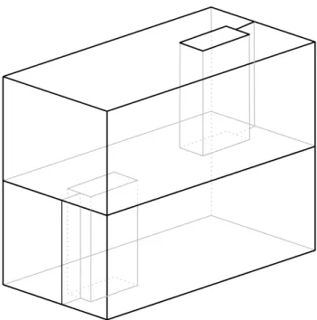
Contact complexes of boxes

The intersection graphs of interior disjoint axis-parallel rectangles in the plane have been studied. Such a contact system of rectangles is said to be proper if at most three rectangles intersect on a point. A tiling is a contact system of axis-parallel rectangles contained in the square [0, 1]_{× [0, 1] such that every} point of the square belongs to at least one of the rectangles. See Figure 1.7 for an example of a box tiling.

Thomassen [103] found a characterization of the intersection graphs of proper tilings, exactly as the strict subgraphs of 4-connected planar triangulations. A natural question which arises is to determine the Dushnik-Miller dimension of intersection complexes of interior disjoint axis-parallel boxes in Rd. Francis and Gon¸calves proved that if the boxes form a “framed tiling” of Rd such that no d + 2 boxes intersect at some point, then the associated intersection complex has Dushnik-Miller dimension at most d + 1 [66].

Cp-orders of orthogonal surfaces

Orthogonal surfaces were introduced by Scarf in [98]. They are defined as fol-lows. Given a finite set of points V in Rd, the orthogonal surface SV is the

topological boundary of the set_{hV i = {x ∈ R}d:_{∃v ∈ V : v}i ≤ xi∀i ∈ [[1, d]]}.

When the considered points do not share coordinates, the points are said to be in general position and the orthogonal surface is said to be generic. For any subset U of V , we define the point pU _{of R}d _{by p}U

i = maxx∈Uxi for every

i∈ [[1, d]]. A characteristic point of a generic orthogonal surface is a point pU

which lies on the orthogonal surface. When equipping the set of these charac-teristic points with the dominance order (where a point x∈ Rd is considered to

(31)

Figure 1.7: Example of a box tiling such that no set of 4 rectangles intersect on a point and its associated intersection graph.

be smaller than another point y_{∈ R}d if and only if xi≤ yifor every i∈ [[1, d]]),

we get the cp-order of a generic orthogonal surface. Scarf showed that cp-orders of some particular generic orthogonal surfaces are isomorphic to the face-lattice of some simplicial d-polytope with one facet removed. Two questions arise from this theorem. First, a realization problem: what are the polytopes whose face-lattice can be seen as a cp-order of some orthogonal surface? Secondly, how to generalize this result to non-generic orthogonal surface? Felsner and Kappes [67] found partial results on these two questions.

1.1.5 Organization of the chapter

In section 2, we prove technical lemmas on representations that are used in the other sections. These lemmas are necessary because any simplicial complex can have different representations. In this section, we prove that the differ-ent represdiffer-entations of a same simplicial complex are connected via elemdiffer-entary operations.

In section 3, we study the Dushnik-Miller dimension of TD-Delaunay plexes. We disprove Conjecture 19 stating that the class of TD-Delaunay com-plexes in Rdcorresponds to the class of Dushnik-Miller at most d + 1 complexes. We provide a counter-example by considering a dual statement.

Section 4 deals with the topology of supremum sections. As we will see in section 3 and 5, supremum sections are connected to some geometric con-figurations. That is why, it is of particular interest to study their topology. Collapsibility is a topological notion introduced by Whitehead [107] which re-sembles shellability and which is defined on any simplicial complex. We prove in this section that any supremum section is collapsible thanks to the discrete Morse theory developed by Forman [68].

In section 5, we study the Dushnik-Miller dimension of contact complexes of stairs, whose shapes in the plane resemble “stairs”. In this study, we consider

(32)

three different arrangements of such stairs which give different results. Partic-ularly, we show that any Dushnik-Miller dimension at most d + 1 complex is a contact complex of stairs.

1.2 Technical lemmas

In this section we prove technical lemmas on representations that will be used in the next section.

Lemma 27(Ossona de Mendez [92]). Let R be a standard d-representation on V . Let X be a face of dimension strictly smaller than d_{− 1 which contains an} interior element of R. Then X is included in two different faces of dimension dim(X) + 1.

Proof. For any i∈ [[1, d]], let xi= max≤i(X) and let Mi= max≤i(V ). Without

loss of generality, suppose that x1 is an interior element of R.

As _{|X| < d, there exists i < j which are indices from [[1, d]] such that} xi= xj= u. By definition of xi and xj, we have x1≤ixi and x1≤jxj. As x1

is an interior element, then Mj<ix1and Mi<j x1. We conclude that u6= Mi

and u_{6= M}j. Furthermore for every k different from i, Mk <ix1≤ixi= u and

for every k different from j, Mk <j x1≤j xj = u and then u6= Mk for every

k_{∈ [[1, d]]. We conclude that u is not an exterior element and that u = x}i<i Mi.

Note that X _6≤k Mi for any k 6= i as x1 is an interior element. We can

therefore define a as the least element according to _≤i such that X <i a and

such that X _6≤k a for every k 6= i. In the same way we define b as the least

element according to _≤j such that X <j b and such that X 6≤k b for every

k6= j. We define Y = XF{a}.

Let us show that Y is a face of Σ(R). First remark that by definition of a, max≤1X = max≤1Y and that every element of X still dominates Y (because

xi = xj is still dominating Y in the order≤j). Furthermore a dominates Y in

the order≤i.

Let u be an element not in Y . As X is a face of Σ(R), there exists k_{∈ [[1, d]]} such that X <k u. Suppose that there exists k0 6= i such that X <k0 u, then

Y <k u. Otherwise k = i, and X 6≤k u. By minimality of a, we have a <k u.

Thus u dominates Y in the order_≤k. We conclude that Y is a face of Σ(R).

Furthermore, by symmetry X_{F{b} is also a face of Σ(R).}

Lemma 28. Let R be a standard d-representation on V and let X be a face of Σ(R) which is included in {M1, . . . , Md} where Mi = max≤iV for every

i ∈ [[1, d]]. The face X is included in one (d − 1)-face. Furthermore, if X ⊆ {M1, . . . , Md} is a (d − 2)-face, then X is included in exactly one (d − 1)-face.

Proof. If there are no interior elements, then the only facet of Σ(R) is the face {M1, . . . , Md} and the proof is clear.

Otherwise, suppose that there exists interior elements. There exists i_{∈ [[1, d]]} such that Mi6∈ X as {M1, . . . , Md} is not a face. We define a as the least element

(33)

Y =_{M1, . . . , Md, a} \ Mi. Let us show that Y is a face of Σ(R). Every element

of Y is dominating Y . As max≤iY = a, every element not in Y is dominating

Y in≤i. We conclude that Y is a (d− 1)-face of Σ(R) which includes X.

Suppose now that X is a (d− 2)-face. Without loss of generality we can suppose that X ={M2, . . . , Md}. Let Y be a (d−1)-face of Σ(R) which contains

X. Then there exists b∈ V different from M2, . . . , Md such that Y = XF{b}.

We note a the least element of V according to ≤i which is not an exterior

element. As a must dominate Y , then Y _≤1 a. We deduce that b≤1 a. As b

cannot be M1(otherwise a could not dominate Y ), then b is an interior element.

By minimality of a, we deduce that a _≤1 b and we conclude that a = b. We

conclude that X is included in exactly one (d_{− 1)-face.}

Corollary 29. For every standard d-representation R on V , Σ(R) is pure of dimensiond_{−1. That means that every face of Σ(R) is included in a (d−1)-face.} Lemma 30. Let R be a d-representation on V such that every element of V is a vertex ofΣ(R). The representation R is standard if and only if there exist verticesM1, . . . Md such that inΣ(R) every face belongs to at least one (d−

1)-face, every(d−2)-face belongs to at least two (d−1)-faces except the (d−2)-faces Fi={M1, . . . , Md} \ Mi which belong to only one (d− 1)-face.

Proof. (=⇒) Clear from Lemma 27 and Lemma 28.

(⇐=) Suppose that there exist vertices M1, . . . , Md such that every face of

Σ(R) belongs to at least one (d_{− 1)-face, and such that every (d − 2)-face} of Σ(R) belongs to at least two (d_{− 1)-faces except the (d − 2)-faces F}i =

{M1, . . . , Md} \ Mi which belong to only one (d− 1)-face.

For any i _{∈ [[1, d]] we define F}0

i as a (d− 1)-face minimizing max≤i(Fi0) in

≤i among the other (d− 1)-faces. Let us denote fi,j0 the element of Fi0 that

is maximal in_≤j. As each of the d elements of Fi0 dominates it at least once,

F0

i ={fi,10 , . . . , fi,d0 }. Let us show that Fi0\ {fi,i0 }, which is a (d − 2)-face, does

not belong to any other (d_{− 1)-face. Indeed, if there exists a vertex x 6= f}0 i,i

such that F0

i \ {fi,i0 } ∪ {x} is a (d − 1)-face then Fi0 <i x by definition of Fi0,

and fi,i0 cannot dominate Fi0\ {fi,i0 } ∪ {x} (as fi,i0 <ix and fi,i0 <j fi,j0 for any

j6= i), a contradiction.

Suppose that there exists i and j6= i such that F0

i\ {fi,i0 } = Fj0\ {fj,j0 }. We

define X = Fi0\ {fi,i0 }. As X is included in Fi0 and in Fj0 , and as it belongs

to only one (d− 1)-face F0

i, we have that Fi0 = Fj0 and thus that fi,i0 = fj,j0 .

Then in the (d− 1)-face F0

i = Fj0, the vertex fi,i0 = fj,j0 thus dominates Fi0 in

two orders, <i and <j, and one of the remaining d− 1 elements of Fi0 cannot

dominate it, a contradiction. We conclude that the faces F0

i\ {fi,i0 } are distinct

and are in bijection with the faces Fi. By symmetry of the Fi0s, we can assume

that Fi= Fi0\ {fi,i0 } and thus that fi,i0 = Mi for every i.

We now show that the Mi’s are the maxima of the representation. Let

i_{∈ [[1, d]] and j 6= i. Since M}i ∈ Fj, none of the (d− 1)-faces is dominated by

Mi in the order≤j. Indeed if it was the case then we would have a (d− 1)-face

F00 _{such that F}00 _≤

j Mi <j fj,j0 (= Mj) which contradicts the definition of Fj0.

Thus F00_≤

(34)

in at least one (d_{− 1)-face, we have that x ≤}iMi. We conclude that Mi is the

maximum of≤i.

We now show that Mi is among the d− 1 smallest elements of the order

≤j for every j 6= i. Since the face Fj contains Mi for every i6= j, none of the

elements in V\ Fj dominates Fj in≤i. Thus each of the|V | − (d − 1) elements

of V\Fjdominates Fj in the order≤j. The element Miis thus among the d−1

smallest elements in order≤j. The representation R is thus standard.

Λ-equivalent representations

The following lemmas are technical and will be useful for the proof of Theorem 44 dealing with TD-Delaunay complexes. The goal here is to study the impact on the representation of an elementary transposition of two consecutive elements in one order of the representation. In the following R is a d-representation (≤1, . . . ,≤d) on a set V and R0 is a d-representation (≤01, . . . ,≤0d) on the same

set V .

Definition 31. Two d-representations R and R0 _are _{Σ-equivalent if Σ(R) =}

Σ(R0_{). Two such representations are Λ-equivalent if, furthermore, for any}

{x, y} ∈ Σ(R), x ≤iy if and only if x≤0iy.

Note that in the case where R and R0 _{are Σ-equivalent, for any i} _{∈ [[1, d]],}

the orders_≤i and≤0i may differ on the comparison of two elements x and y if

{x, y} 6∈ Σ(R) = Σ(R0_).

Given a d-representation R, an (≤i)-increasing xy-path is a path (x =

a0, a1, a2, . . . , ak = y) in Σ(R) such that aj ≤i aj+1 for every 0 ≤ j < k.

Given two Λ-equivalent d-representations R and R0, note that a path P is (≤i

)-increasing (in Σ(R)) if and only if it is (≤0

i)-increasing (in Σ(R0)). Note also

that for any face F ∈ Σ(R), max≤i{x ∈ F } = max≤0_i{x ∈ F }.

Definition 32. LetR = (_≤1, . . . ,≤d) be a d-representation on V . Let x and y

be two distinct vertices of Σ(R) (i.e. _{{x} and {y} ∈ Σ(R)) such that {x, y} 6∈} Σ(R) and such that x and y are consecutive in an order _≤i. We defineR0 =

(_≤0

1, . . . ,≤0d) the d-representation on V obtained after the permutation of x and

y in the order i. We say that we obtained R0 _{by an} _{elementary transposition.}

Lemma 33. Two d-representations on V , R = (≤1, . . . ,≤d) and R0 = (≤01

, . . . ,≤0

d), are Λ-equivalent if and only if R0 can be obtained from R after a

sequence of elementary transpositions.

Proof. Let us first prove that if R0_{is obtained from R by an elementary}

transpo-sition of x and y in the order_≤1(with x≤1y), then these two representations

are Λ-equivalent.

We first prove that these two representations are Σ-equivalent. Towards a contradiction and by symmetry of R and R0_{, let us consider a face F} _{∈ Σ(R)}

such that F _{6∈ Σ(R}0_{). There exists therefore a vertex z} _{∈ V which does not}

dominate F in R0_{. As z dominates F in R, and as} _≤

i≡≤0i for every i6= 1, we