Bauwens : Université Catholique de Louvain, CORE, B-1348 Louvain-la-Neuve.
Rombouts : Institute of Applied Economics at HEC Montréal, CIRANO, CIRPÉE and CORE (Université Catholique de Louvain). Research supported by the contract “Projet d’Actions de Recherche Concertées” 07/12-002 of the “Communauté française de Belgique”, granted by the “Académie universitaire Louvain”. Bauwens is also a member of ECORE, an association between ECARES and CORE. This text presents research results of the Belgian Program on Interuniversity Poles of Attraction initiated by the Belgian State, Prime Minister’s Office, Science Policy Programming. The scientific responsibility is assumed by the authors. Cahier de recherche/Working Paper 09-42
On Marginal Likelihood Computation in Change-Point Models
Luc Bauwens
Jeroen V.K. Rombouts
Abstract:
Change-point models are useful for modeling times series subject to structural breaks. For interpretation and forecasting, it is essential to estimate correctly the number of change points in this class of models. In Bayesian inference, the number of change-points is typically chosen by the marginal likelihood criterion, computed by Chib’s method. This method requires to select a value in the parameter space at which the computation is done. We explain in detail how to perform Bayesian inference for a change point dynamic regression model and how to compute its marginal likelihood. Motivated by our results from three empirical illustrations, a simulation study shows that Chib’s method is robust with respect to the choice of the parameter value used in the computations, among posterior mean, mode and quartiles. Furthermore, the performance of the Bayesian information criterion, which is based on maximum likelihood estimates, in selecting the correct model is comparable to that of the marginal likelihood.
Keywords: BIC, Change-point model, Chib’s method, Marginal Likelihood
1
Introduction
Economic and financial time series are subject to changes in their pattern over long periods, see e.g. Stock and Watson (1996) for US macroeconomic data, Pastor and Stambaugh (2001) and Liu and Maheu (2008) for financial series. It is therefore interesting to take into account the possibility of structural change in time series models, both for interpreting historical data and for forecasting future values. Researchers do not usually assume that break dates are known. Models allowing for the possibility of changing structure or parameters have thus been developed over the last twenty years. In particular, the change in model parameters can be modelled by a Markov-switching discrete process, following the impetus given by Hamilton (1989). The states of this process, which correspond to the parameter values, are recurrent as the process can move from one state to any other state at any date. A particular case of this model is the change-point model that has non-recurrent states: the process can only stay in the same state or move to the next one. An important and difficult issue is the choice of the number of states of the hidden Markov chain, since this determines the number of structural breaks in the time series. For this issue, Bayesian inference is useful: one can estimate the model for a range of values of the number of states and choose the model that delivers the highest marginal likelihood. When maximum likelihood estimation is feasible, one can likewise choose the model according to the Bayesian (or Schwarz) information criterion (BIC).
The computation of the marginal likelihood of a given Markov-switching model can be performed by the method of Chib (1995). This method only uses the Gibbs output, while other methods like those Newton and Raftery (1994) and Gelfand and Dey (1994) are either unstable or need an additional tuning function. Chib’s method is based on the marginal likelihood identity, namely that the marginal likelihood is equal to the product of the likelihood and the prior divided by the posterior. Since each element on the right hand side of this identity depends on the model parameters, a particular value must be chosen, even if the result does not depend in principle on this value. Chib recommends to choose a high posterior density value for numerical efficiency reasons. Many researchers use the posterior mean, see e.g. Kim and Nelson (1999), Elerian, Chib, and Shephard (2001), Kim and Piger (2002), Kim, Morley, and Nelson (2005), Pesaran, Pettenuzzo, and Timmermann (2006), Johnson and Sakoulis (2008), Liu and Maheu (2008), Maheu and Gordon (2008), Fruhwirth-Schnatter and Wagner
(2008), Nakajima and Omori (2009), and few, such as Paroli and Spezia (2008), use the mode. To the best of our knowledge, no study has clearly documented the sensitivity of the marginal likelihood value obtained by Chibs’ method to the value of the parameter chosen for its computation in the case of Markov-switching models.
The first goal in this paper is precisely to assess this sensitivity in the case of a change-point regression model. As mentioned above, change-change-point models are a particular case of Markov-switching models. In the general case of recurrent states, the number of parameters of the transition matrix of the Markov chain is equal to K2− K, where K is the number of states. A change-point model is much more parsimonious in this dimension since it requires only K − 1 parameters. Even if a change-point model may require a higher K than a general Markov-switching one, it is not likely that the number of change points will be as high as
K2− K. Another advantage of change-point models is the fact that they are not subject to the label switching problem of general Markov-switching models, which renders estimation much more difficult.
Based on a simulation study, our conclusion is that Chib’s method is not much sensitive to the chosen value of the parameter for computing the marginal likelihood, and we recom-mend to use indifferently the posterior mode, mean or median rather than other values. Our simulation study is based on three change-point regression models whose specification and parameter values are closely inspired by models that we estimated using real time series.
Moreover, for models of the type we consider, Chib’s method uses, as always, the output of the Gibbs sampler, but requires additional simulations due to the presence of the latent variables. This explains, at least partially, why computations are typically heavy. The second objective of this paper is to compare the model choices resulting from the application of the BIC and of the marginal likelihood criterion. Computing the BIC requires of course to maximize the log-likelihood function, which is not an easy task when the number of change points is large, the reason being the existence of multiple local maxima. The simulation results show that the BIC leads to choose the correct model in a higher proportion of replications than the marginal likelihood criterion, and that a correct computation of the BIC is not necessarily less heavy than for the marginal likelihood.
The paper is structured as follows: in Section 2, we present change-point models and how Bayesian inference is done. This is done in detail so as to make the presentation, done in
Section 3, of the computation of the marginal likelihood and BIC understandable. Section 4 contains the empirical examples and Section 5 the simulation results. Section 6 concludes.
2
Model and inference
In Section 2.1 we explain how breaks can be introduced in a time series model, drawing on the work of Chib (1998) and Pesaran, Pettenuzzo, and Timmermann (2006). In Section 2.2, we define the prior densities, and in Section 2.3, we explain how to compute the posterior density of the parameters of this type of model by Gibbs sampling.
Concerning notations, we adopt some conventions: by default vectors are columns and
y0 denotes the transpose of y. Data densities (including predictive) for observable or latent variables, whether discrete or continuous, are denoted by f (.). Prior and posterior densities are denoted by ϕ(.). Parameters of prior densities are identified by underscore bars (e.g. a), those of posterior densities by overscore bars (e.g. a).
2.1 Model
Let yt be the time series we want to model over the sample period {1, 2, . . . , T }. Let st be an integer latent variable (also called state variable) taking its value in the set {1, 2, . . . , K},
K being assumed known. The state variable st indicates the active regime generating yt at period t in the sense that ytis generated from the data density
f (yt|Yt−1, θst), (1)
where Yt−1 = (Y00 y1 . . . yt−1)0, Y0 being a vector of known initial conditions (observations prior to date t = 1), and θst is a vector of parameters indexing the density. There are potentially K regimes, hence K parameter vectors θ1, θ2, . . . , θK.
We assume that the active regime at t is selected by a discrete first-order Markov process for the st process. As in Chib (1998), the transition probability matrix PK (more simply denoted by P when indicating the number of regimes is not important) allows either to stay in the regime operating at t−1 or to switch to the next regime and has therefore the following
structure: PK = p11 1 − p11 0 . . . 0 0 0 p22 1 − p22 . . . 0 0 .. . ... ... ... ... ... 0 0 0 . . . pK−1,K−1 1 − pK−1,K−1 0 0 0 . . . 0 1 . (2)
Notice that the last regime is an absorbing state over the sample period. Given the zero entries in P , the discrete Markov chain generates potentially K − 1 breaks, at random dates
τk (k = 1, 2, . . . , K − 1) defined by τk being the integer in {1, 2, . . . , T } such that sτk = k and sτk+1 = k + 1. A posterior density on these dates is therefore a direct by-product of the inference on the state variables. A convenient prior density, based on the assumption of independence between the parameters of the matrix P , takes the form of a product of identical beta densities with parameters a and b:
ϕ(p11, p22, . . . , pK−1,K−1) ∝ K−1Y
i=1
pa−1ii (1 − pii)b−1. (3) The assumption that the beta densities are identical can be easily relaxed. This prior implies that the (strictly positive integer) duration of regime k, dk = τk− τk−1 (setting τ0 = 0 and
τK = T ) is approximately geometrically distributed with parameter pii and expected value (a+b)/a. For example, by fixing a = b = 1, the prior is uniform for each probability. Actually, fixing a = b implies that E(dk) = 2 and a priori, on average, a lot of regimes. To choose a prior on the probabilities consistent with K, T /K should be the expected number of observations per regime. Hence one should fix E(pii) = 1 − (K/T ), which implies that a/b = K/(T − K) and fixes one of the parameters given the other. The other parameter can be deduced by fixing the variance of the beta distribution and solving.1
Following Pesaran, Pettenuzzo, and Timmermann (2006), an essential ingredient of the model specification is the prior assumption that the parameter vectors θi are drawn indepen-dently from a common distribution, i.e. θi ∼ ϕ(θi|θ0) where θ0 itself is a parameter vector
1If one substitutes bK/(T − K) for a in v = ab/[(a + b)2(a + b + 1)] where v is the assigned prior variance,
endowed with a prior density ϕ(θ0|A), A denoting the prior hyper-parameters. This is called a hierarchical prior or a meta-distribution. For example, if θi contains location parameters and a scale one, the prior can be a normal density on the location parameters and a gamma density on the scale one. Generally, the joint prior on the θ parameters is
ϕ(θ0, θ1, θ2, . . . , θK) = ϕ(θ0|A) K Y i=1
ϕ(θi|θ0). (4)
Behind the common prior (4) lies the belief that the regime parameters differ and evolve independently of each other. Another possible prior belief is that the regime parameters evolve in a more structured way. For example the conditional mean of ytcould be increasing (µk−1 < µk). This idea can be formalized through a joint normal prior on (µ2− µ1, µ3−
µ2, . . . , µK− µK−1)0 with mean vector m
0ιK−1 and covariance matrix V0, where m0 and V0 are the hyper-parameters to be endowed with a prior density implying that m0 is positive with high probability.
The model is fully specified by defining the conditional densities f (yt|Yt−1, θst). In this study, we use the following assumption:
yt|Yt−1, θst ∼ N (xt0βst, σs2t), (5)
where xt is a vector of m exogenous variables and βst a vector of coefficients, so that θst = (βs0tσ2st)0. In our applications, the model within a regime is autoregressive, i.e. xt includes the constant 1 and p lags of yt, hence m = p + 1.
2.2 Prior densities for location and scale parameters
In the model developed in the previous sub-section, the hierarchical prior (4) is defined by a prior for each βj (j = 1, 2, . . . , K) and an independent prior for each σj2, given additional random parameters (forming θ0) defined below, to which prior densities are assigned. The hierarchy can be divided into two independent pieces, one for the regression coefficients and one for the variances. We define the two pieces, provide the formulas of some moments, and discuss how to define weakly informative (proper) prior densities. Improper prior densities are excluded as we want to compute the marginal likelihood.
Regression coefficients The hierarchical prior is
βj|b0, B0 ∼ Nm(b0, B0), (6)
b0 ∼ Nm(µβ, Σβ), (7)
B0−1 ∼ Wm(υβ, V−1β ), (8)
with b0 independent of B0. Wm(ν, S) denotes a Wishart density of dimension m with scale parameter S, a positive-definite symmetric matrix, and ν degrees of freedom (ν > m − 1). If m = 1, this reduces to a Gamma(ν, s) defined below, see (14). Equivalently, B0 has an inverted Wishart density, B0 ∼ IWm(ν, S), see Appendix A of Bauwens, Lubrano, and Richard (1999), with E(B0) = V−1β /(υβ− m − 1) if υβ > m + 1. Although the prior marginal density of βj is not known analytically, its moments can be obtained by applying the law of iterated expectations:
E(βj) = µβ, (9)
Var(βj) = E(B0) + Var(b0) =
V−1β
υβ − m − 1+ Σβ if υβ > m + 1. (10)
To be weakly informative on the βj parameters, one usually sets B−10 close to 0 and diagonal in (6), meaning the variances are large and the elements are independent, and
b0 = 0, though taking another value does not matter if B0−1 close to 0. In our hierarchical setup one can set µβ = 0 instead of b0 = 0. In view of (10), one can achieve large variances through Var(b0) or E(B0). It is more direct and easier for understanding the prior to make Var(b0) large, rather than E(B0). For Var(b0), this means setting Σβ = c1Im with a large value of c1, but what ”large” means has to be considered relatively to the order of magnitude of the βj parameters. We set υβ = m + 2 and Vβ = Im, such that E(B0) = Im.
Variances
The hierarchical prior is defined as
σj−2|υ0, d0 ∼ Gamma(υ0, d0), (11)
υ0 ∼ Gamma(λ0, ρ0), (12)
with υ0 independent of d0. We use the following definition of a Gamma(ν,s) density for x where ν is the degrees of freedom and s is the scale parameter:
fG(x|ν, s) =³ s2 ´ν 2 h Γ³ ν 2 ´i−1 xν2−1exp ³ −s 2x ´ for x > 0. (14) Its expected value is ν/s and its variance is 2ν/s2. Equivalently to (11), and using the terminology of Bauwens, Lubrano, and Richard (1999), σ2
j has an inverted gamma-2 density,
σ2 j|υ0, d0∼ IG(υ0, d0), with E(σ2j|υ0, d0) = d0/(υ0− 2) if υ0 > 2, (15) Var(σ2j|υ0, d0) = 4d 2 0 (υ0− 2)2(υ0− 4) if υ0 > 4. (16) The prior marginal density of σj−2 (or its inverse) cannot be computed analytically, but its expectation can:
E(σ−2j ) = E(υ0)E(d1 0
) = λ0
ρ0 d0
c0− 2if c0 > 2. (17)
Note however that E(σ2
j) does not exist since υ0 < 2 has a non-zero probability if υ0 ∼ Gamma(λ0, ρ0).
The non-informative version of a prior density on a variance σ2
j is usually taken as ϕ(σ2j) ∝ 1/σ2
j or equivalently ϕ(σ−2j ) ∝ 1/σj−2. This corresponds to setting υ0 = d0= 0. This approach is not feasible when υ0 and d0 are random variables. The same type of non-informative prior for υ0 and d0 is obtained by setting their hyper-parameters at 0. This implies that E(σj−2) does not exist. The full conditional posterior density of d0 is still a proper density even if
c0= d0 = 0 since it is a Gamma(Kυ0+ c0, PK
j=1σj−2+ d0), as shown in the next sub-section. The latter result suggests that d0 should not dominate the sum of the inverted variances if one wishes to be weakly informative on d0. Setting the prior degrees of freedom c0 is more difficult since it is added to Kυ0 which is random. The prior mean of Kυ0, equal to Kλ0/ρ0, can serve as reference value to fix c0. As PPT, we set c0 = 1 and d0= 0.01, hence E(d0) = 100 and Var(d0) = 20000.
In the next sub-section where the Gibbs algorithm is described, it is shown that the full conditional posterior density of υ0 does not belong to a known class of density functions. Hence it is not possible to compare the hyper-parameters λ0 and ρ0 to their counterparts from the information set. We set λ0 = 1 and ρ0 = 0.01, so that the prior mean and standard deviation of υ0 are both equal to 100, such that our prior densities are weakly informative
2.3 Inference
The joint posterior density of ST = (s1 s2 . . . , sT)0 and the parameters is proportional to T Y t=1 f (yt|Yt−1, θst)f (st|st−1, P ) K−1Y i=1 pa−1ii (1 − pii)b−1 K Y i=1 ϕ(θi|θ0) ϕ(θ0|A), (18)
where f (st|st−1, P ) is the transition probability from state t − 1 to state t and is one of the
non null elements of P . The parameters are θi, i = 0, 1, . . . , K, jointly denoted by Θ (or ΘK to emphasize that K regimes are assumed), and the diagonal elements of the matrix P . This density lends itself to simulation by Gibbs sampling in three blocks corresponding to the full conditional densities: 1. ϕ(ST|Θ, P, YT) ∝ QT t=1f (yt|Yt−1, θst)f (st|st−1, P ), 2. ϕ(P |ST) ∝ QT t=1f (st|st−1, P ) QK−1 i=1 p a−1
ii (1 − pii)b−1, which does not depend on Θ and
YT, and
3. ϕ(Θ|ST, YT) ∝QTt=1f (yt|Yt−1, θst) QK
i=1ϕ(θi|θ0) ϕ(θ0|A), which does not depend on P . Sampling ST is done as Chib (1998) and detailed below (notice that sT = K by assump-tion). Sampling P is done by simulating each pii from a beta density with parameters a + Ti and b + 1 where Ti is the number of states equal to i in the sampled ST vector. Sampling Θ implies usually to break it into sub-blocks and to sample each sub-block given the other, plus
ST. We give all the necessary details below for the case when f (yt|Yt−1, θst) is the normal density defined in (5).
Chib’s algorithm for sampling the states
The algorithm is explained in Chib (1996) for the case when the matrix P is not restricted and in Chib (1998) for the case when P is restricted like in (2), but the differences between the two cases are minor. The state vector ST is sampled from ϕ(ST|Θ, P, YT), by sampling sequentially from T to 1 using the backward sequential factorization
ϕ(sT −1|sT, YT, Θ, P ) . . . ϕ(st|st+1, YT, Θ, P ) . . . ϕ(s2|s3, YT, Θ, P ) (19)
and the fact that the model structure implies that sT = K and s1 = 1 with probabil-ity 1. In the above factorization, ϕ(st|st+1, YT, Θ, P ) should in principle be replaced by
ϕ(st|st+1, st+2, . . . , sT, YT, Θ, P ), but the added conditions st+2, . . . , sT are not needed since
ϕ(st|st+1, st+2, . . . , sT, YT, Θ, P ) ∝ f (st|Yt, Θ, P )f (st+1|st, P ), (20) which also shows that ϕ(st|st+1, YT, Θ, P ) = ϕ(st|st+1, Yt, Θ, P ). Indeed, as in equation (7) in Chib (1996), and using the notation St+1= (s
t+1st+2 . . . sT) and similarly for Yt+1,
ϕ(st|St+1, YT, Θ, P ) ∝ f (st|Yt, Θ, P )f (Yt+1, St+1|Yt, st, Θ, P ) (21)
∝ f (st|Yt, Θ, P )f (st+1|st, P )f (Yt+1, St+2|Yt, st, st+1, Θ, P ) (22) ∝ f (st|Yt, Θ, P )f (st+1|st, P ). (23) The first line (21) follows from
ϕ(st|St+1, YT, Θ, P ) ∝ f (st, St+1|Yt, Yt+1, Θ, P )
∝ f (st, St+1, Yt+1|Yt, Θ, P )
∝ f (st|Yt, Θ, P )f (St+1, Yt+1|st, Yt, Θ, P ). For (22),
f (Yt+1, St+1|Yt, st, Θ, P ) = f (st+1|Yt, st, Θ, P )f (Yt+1, St+2|st+1, Yt, st, Θ, P )
and f (st+1|Yt, st, Θ, P ) = f (st+1|st, P ) from the model assumption about the Markov chain for the states. The third line (23) follows from from the fact that the third factor of the rhs of the second line does not depend on st.
One starts with generating a random draw from ϕ(sT −1|sT = K, YT −1, Θ, P ), then
con-tinues with ϕ(sT −2|sT −1, YT −2, Θ, P ) where sT −1 is set equal to the random draw generated from the previous factor, and so on until s2 is generated. Actually, ϕ(st|st+1, Yt, Θ, P ) can only take two values given the structure of P in (2), therefore one can just compute these two values according to the rhs of (20) and divide by their sum to obtain normalized probabilities. In the rhs of (20), f (st+1|st, P ) is the same as in (18), and f (st|Yt, Θ, P ) is computed by recurrence from f (st−1|Yt−1, Θ, P ). One starts at t = 2 with initial condition f (s1|Y1, Θ, P ) = 1 if s1 = 1 and = 0 otherwise (at t = 1, only state 1 can occur), and one ends at T − 1 since
f (sT|YT, Θ, P ) = 1 if sT = K and = 0 otherwise. The passage from f (st−1|Yt−1, Θ, P ) to
Prediction step: by the law of total probability, f (st|Yt−1, Θ, P ) = K X j=1 f (st|st−1= j, P )f (st−1= j|Yt−1, Θ, P ), (24) given that f (st|st−1= j, P ) = f (st|st−1= j, Yt−1, Θ, P ) from the assumptions on the model. Update step: by Bayes theorem,
f (st|Yt, Θ, P ) ∝ f (st|Yt−1, Θ, P )f (yt|Yt−1, Θst), (25)
which is easily normalized by dividing by the sum of the rhs over all values of st (even if actually the rhs is strictly positive only for two values of st).
Gibbs algorithm for Θ
Given (5), yt|Yt−1∼ N (x0tβj, σ2j) when st= j. The prior densities are given in (6)-(8) and (11)-(13). The parameters are divided into 4 + 2K blocks: b0, B0, υ0, d0(altogether corresponding to θ0 in (4)), βj, and σj2 (for each j = 1, . . . , K). We provide the conditional posterior density of each block (given the relevant other parameters and the state vector ST when it is needed). Each of these is obtained by keeping all parts of QTt=1f (yt|Yt−1, θst)
QK
i=1 ϕ(θi|θ0) ϕ(θ0|A) that depend on the relevant elements. The hyperparameter A corresponds to the parameters of (7), (8), (12), and (13). Given ST, we assign each observation to one of the K regimes and thus we form K vectors yj and matrices Xj that contain the yt and x0tobservations assigned to regime j. We denote by Tj the number of observations assigned to regime j. Below we state the result for each block and sketch how we obtain it.
• For each j = 1, . . . , K: βj|σj2, b0, B0, ST, YT ∼ Nm( ¯βj, ¯Vj), where ¯Vj = (σ−2j Xj0Xj+ B0−1)−1 and ¯βj = ¯Vj(σj−2Xj0yj+ B0−1b0). Indeed, denoting ˆβj = (Xj0Xj)−1Xj0yj,
p(βj|σ2j, b0, B0, ST, YT) ∝ exp −0.5[(βj− b0)0B0−1(βj− b0) + σ−2j (yj− Xjβj)0(yj− Xjβj)]
∝ exp −0.5[(βj− b0)0B0−1(βj− b0) + σ−2j (βj− ˆβj)0Xj0Xj(βj− ˆβj)]
∝ exp −0.5[(βj− ¯βj)0V¯j−1(βj− ¯βj).
• For each j = 1, . . . , K: σ−2j |βj, υ0, d0, ST, YT ∼ Gamma(υ0+Tj, d0+(yj−Xjβj)0(yj−Xjβj)), since
p(σ−2j |βj, υ0, d0, ST, YT) ∝ (σ−2j )υ0/2−1 exp[−0.5σj−2d0] (σ−2j )Tj/2 exp[−0.5σ−2
• b0|β1, . . . , βK, B0, YT ∼ Nm(¯µβ, ¯Σβ), where ¯Σβ = (Σ−1β + KB−10 )−1 and ¯µβ = ¯Σβ(Σ−1β µβ+
B0−1PKj=1βj). This comes from
p(b0|β1, . . . , βK, B0, YT) ∝ exp[−0.5(b0− µβ)0Σ−1β (b0− µβ)] K Y j=1 exp[−0.5(βj − b0)0B0−1(βj− b0)]. • B0−1|β1, . . . , βK, b0, YT ∼ Wm(νβ, V−1β ), where νβ = νβ + K and V −1 β = V−1β + PK j=1(βj− b0)(βj− b0)0. Indeed, p(B0−1|β1, . . . , βK, b0, YT) ∝ |B0−1| νβ+m+1 2 exp[−0.5trB−1 0 V−1β ] K Y j=1 |B0|−1/2exp[−0.5(βj− b0)0B0−1(βj− b0)] ∝ |B0−1|νβ+K+m+12 exp[−0.5trB−1 0 (V−1β + K X j=1 (βj− b0)(βj− b0)0]. • d0|σ1, . . . , σK, υ0, YT ∼ Gamma(c0+ Kυ0, d0+ PK j=1σ−2j ), since p(d0|σ1, . . . , σK, υ0, YT) ∝ dc00/2−1 exp[−0.5d0d0] K Y j=1 dυ0/2 0 exp[−0.5d0σj−2]. • υ0|σ1, . . . , σK, d0, YT ∝ fg(υ0|λ0, ρ0) QK
j=1fg(σ−2j |υ0, d0). Since this is not belonging to a known class of densities, we simulate it by inverting numerically its cdf computed by Simpson’s rule (rather than using a a Metropolis algorithm as PPT do).
3
Marginal likelihood and BIC computation
In this section, we give details about the computation of the marginal log-likelihood (MLL) and the Bayesian information criterion (BIC). We are interested by the following questions:
1. Is the value of the MLL computed by Chib’s algorithm reliable?
2. If we apply the BIC to choose the number of change points, do we get approximately the same results as if we apply the MLL criterion?
Answers to these questions are provided in Sections 4 and 5. The motivation for using the BIC is that it is well known, and in large samples it usually leads to choose the model also picked
by the MLL criterion, see the discussion in Kass and Raftery (1995). The BIC is generally more quickly programmed and computed than the MLL. For the change-point models we consider, this is especially true in terms of programming time. Once a correct computer program is available, only computing time matters, and in that respect computing the BIC is not necessarily quicker than computing the MLL, because obtaining the global maximum of the log-likelihood function may require many computations (see below).
3.1 Marginal likelihood
The posterior density defined in (18) is conditional on a known value of K, the number of regimes in the sample period. Obviously, K can range from 1, the no break scenario, to T (the sample size). The latter case can be interpreted as a time-varying parameter (TVP) model, for which one often assumes θi = θ0+ Φθi−1+ vt where θ0, Φ are parameters (often set equal to 0 and I, respectively) and vtis a multivariate normal vector with zero mean and unknown covariance matrix.
We can choose the model corresponding to the value of K that maximizes the marginal likelihood (also called predictive density) of the sample. We can also use model averaging, over a range of values of K, say K ∈ {1, 2, . . . , ¯K} where ¯K is the largest number of regimes that
we wish to consider. Model averaging requires posterior model probabilities, which themselves require prior model probabilities and the marginal likelihood value for each model.
To compute the marginal log-likelihood for the data YT and the model MK with parame-ters ΘK = (θ0, θ1, . . . , θK) and PK = (p11, p22, . . . , pK−1,K−1) defined in the previous section, we use the idea of Chib (1995). The predictive density is related to the prior, posterior and data density by the equality
f (YT|MK) = f (YT|MK, ΘK, PK)ϕ(ΘK, PK|MK)/ϕ(ΘK, PK|MK, YT).
Since this holds for any admissible parameter value, we can pick a value (Θ∗K, PK∗) of the parameters and compute
log f (YT|MK, Θ∗K, PK∗) + log ϕ(Θ∗K, PK∗|MK) − log ϕ(Θ∗K, PK∗|MK, YT) (26) to approximate log f (YT|MK). Notice that all densities in the above equation must be proper (i.e. integrate to 1), hence the requirement to use a proper prior. In principle, (Θ∗
can be any value in the parameter space, but the posterior mean or mode is an easy and recommended choice. In Sections 4 and 5, we report results throwing light on the sensitivity of the value of the marginal log-likelihood with respect to the value of Θ∗
K.
The first term in (26) is the log-likelihood function of the model, which can be written as log f (YT|MK, Θ∗K, PK∗) = T X t=1 log f (yt|YT −1, Θ∗K, PK∗) (27) where f (yt|YT −1, Θ∗K, PK∗) = K X j=1 f (yt|Yt−1, Θ∗K, PK∗, st= j)f (st= j|Yt−1, Θ∗K, PK∗). (28) In each term of the above sum, the first factor is equivalent to f (yt|Yt−1, θ∗j) and the second is obtained by the prediction step of Chib’s algorithm, see (24). Actually, the log-likelihood function does not depend on θ∗
0.
The prior density is defined analytically and easily computed. The difficult part is the computation of the log-posterior since it must be computed numerically. We use the factor-ization ϕ(Θ∗K, PK∗|MK, YT) = ϕ(Θ∗K|MK, YT)ϕ(PK∗|Θ∗K, MK, YT), (29) where ϕ(PK∗|Θ∗K, MK, YT) = Z ϕ(PK∗|MK, YT, ST)ϕ(ST|Θ∗K, MK, YT)dST since PK is independent of ΘK given ST. This is estimated by
H−1 H X h=1 ϕ(PK∗|MK, YT, ST,h), where {ST,h}H
h=1are H draws generated from the Gibbs sampler described in sub-section 2.3,
conditioned on Θ∗, i.e. it iterates between ϕ(S
T|Θ∗, P, YT) and ϕ(P |ST). The first density in the right-hand side of (29) can be expressed as
ϕ(Θ∗K|MK, YT) = Z ϕ(Θ∗K|MK, YT, ST)ϕ(ST|MK, YT)dST. It could be estimated by G−1 G X g=1 ϕ(Θ∗K|MK, YT, ST,g), (30)
where {ST,g}Gg=1are G draws generated from the posterior density through the Gibbs sampler described above, if ϕ(Θ∗K|MK, YT, ST,g) were known analytically. However this is not typically the case. To solve this problem, we partition Θ∗
K in B blocks {Θ∗K,b}Bb=1, such that the full conditional posterior densities ϕ(Θ∗K,b|MK, YT, ST, {Θ∗K,c}c6=b) are known analytically or if not can be computed by numerical integration. These blocks are those used for implementing step 3 of the Gibbs sampler (see sub-section 2.3). Then, we factorize ϕ(Θ∗K|MK, YT) as
ϕ(Θ∗K,1|MK, YT)ϕ(Θ∗K,2|MK, YT, Θ∗K,1) . . . ϕ(Θ∗K,B|MK, YT, Θ∗K,1, . . . , Θ∗K,B−1),
and we implement an auxiliary Gibbs sampler to compute each density of this factorization in the same way as (30). For example, ϕ(Θ∗
K,2|MK, YT, Θ∗K,1) is estimated as G−1 G X g=1 ϕ(Θ∗K,2|MK, YT, ST,g, Θ∗K,1, ΘK,3,g, . . . , ΘK,B,g)
where {ST,g, ΘK,3,g, . . . , ΘK,B,g}Gg=1are draws from the auxiliary Gibbs sampler. This sampler is the one defined in sub-section 2.3 conditioned on Θ∗
K,1 and Θ∗K,2.
In the context of the normal regression model (5) for each regime, B = 6 and ΘK,1 corresponds to the K vectors βj, ΘK,2 to the K parameters σj−2, ΘK,3 to b0, ΘK,4 to B−10 , ΘK,5 to d0, and ΘK,6 to υ0. This way of partitioning ΘK minimizes the computational time by exploiting the conditional independence features of the posterior, since the the last four blocks do not require integration with respect to the states. The last block is reserved for υ0 since it requires numerical integration that can be done only once since the other parameters are then fixed.
3.2 BIC
To compute the BIC, we must of course compute the maximum likelihood estimator since we need to evaluate the log-likelihood at its maximum and penalize it by the usual term 0.5mKlog T , where mKis the number of parameters of model MK. The log-likelihood function of the change-point model is given in (27)-(28). We maximize it by a gradient method (algorithm BFGS of Ox). There may be several local maxima. Thus we maximize the objective function many times, using different starting values. We choose them as follows: for a given number of change points, we draw randomly the break dates, taking care that each regime has at least 30 observations, and given these dates, we estimate the model by
OLS in each regime, thus obtaining starting values for the autoregressive coefficients and the variance of the error. The starting values for the transition probabilities pkk are set to 0.98 or 0.99, since transitions are not frequent. For the applications reported in the next section, we did 100 maximizations and chose as value of the log-likelihood for computing the BIC the maximum of the 100 log-likelihood values. For the simulation results in Section 5, we used 20 maximizations in each experiment.
For running the Gibbs sampler, we use as starting values the MLE values used for com-puting the BIC.
4
Empirical examples
In this section, we apply the change-point model to three time series. Our empirical results serve to motivate and design the simulation experiments reported in the next section. 4.1 Quarterly growth rate of US GDP
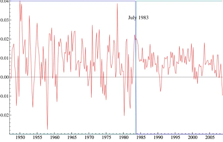
The sample for this series covers the period from the first quarter of 1947 to the last one of 2008 (248 observations). The original series of the real GDP is seasonally adjusted. It was down-loaded from the web site of the Federal Reserve Bank of St. Louis (http://alfred.stlouisfed.org/, series GDPC1 20090130). The growth rate series is plotted in Figure 6.
We use an AR(p) model in each regime, with p ≤ 4. We limit the number of regimes to be equal to 3 at most. According to the BIC and MLL criteria, the best model is an AR(1) with two regimes. Table 1 reports, for p = 1, the BIC and several MLL values, obtained by applying formula (26) for different parameter values: posterior means, mode, medians, 0.25-quantiles, and 0.75-quantiles, where the quantiles are from each marginal distribution. The choice of two regimes is consistent across the BIC and all values of the MLL. The latter hardly differ for each K. The posterior means, standard deviations, mode, medians and other quantiles of the main parameters of the best model are reported in Table 2. The posterior median of the break date is 1983, second quarter (July) as shown in Figure 6. The break corresponds to a large reduction of the error variance and is called ”the great moderation” by economists. The persistence parameter of the AR(1) hardly changes after the break.
4.2 Monthly growth rate of US industrial production
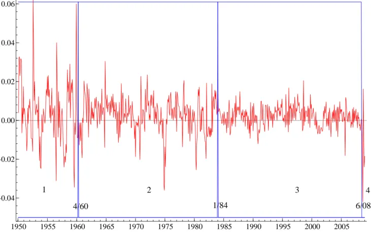
The sample for this series covers the period from January 1950 to January 2009 (709 obser-vations). The original series, downloaded from Datastream (USIPTOT.G series), is a volume index of the industrial production of the USA and is seasonally adjusted, equal to 100 in 2002. We work with the growth rate series, plotted in Figure 6, defined as the first difference of the logarithm of the original series.
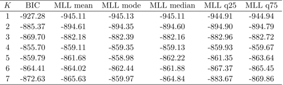
We use an AR(1) model in each regime. We limit the number of regimes to be equal to 7 at most. According to the BIC and MLL criteria, the best model has four regimes, see Table 3. The choice of four regimes is consistent across the BIC and the values of the MLL with the exception of the MLL evaluated at the mode which leads to select K = 5. One can notice that differences between the criteria values between 3 and 4 regimes are much more important than between 4 and 5.
The MLL values hardly differ for each K. The posterior central values, standard devia-tions, and 0.25/0.75 quantiles of the main parameters of the best model are reported in Table 4. The posterior medians of the break dates are April 1960, January 1984, and June 2008, as shown in Figure 6. The first break corresponds to a large reduction in the variance of the growth rate: the posterior mean of the residual variance is divided by three. The second break corresponds to a further reduction (division by 2.5). The last break corresponds clearly to the big recession triggered by the subprime crisis of 2007, with a huge increase of the residual variance. The coefficients of the AR(1) equation are very similar in the first two regimes, and change a lot in the last two regimes though the precision of the estimation for the last regime is low due to the very small number of observations.
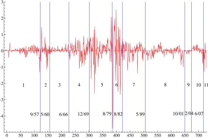
4.3 Monthly US 3-month T-bill rate
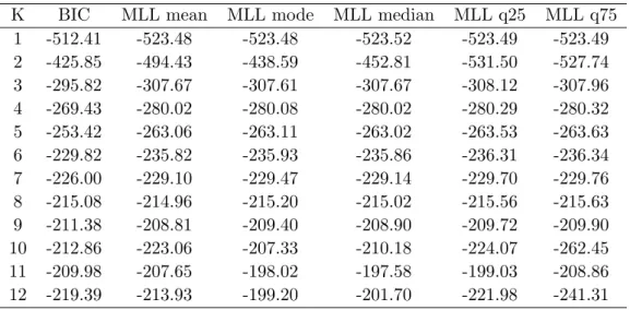
This monthly series was analyzed by Pesaran, Pettenuzzo, and Timmermann (2006) using an AR(1) model for the level. We extend the sample by almost five years, covering the period July 1947 to September 2008 (735 observations). The estimation results for an AR(1) model indicate that most of the regimes are nearly integrated. Therefore, we use an AR(0) model for the first difference. The series (from the CRSP database) is shown in Figure 6, together with the regimes resulting from the detected break dates (posterior medians of change points). The number of regimes is equal to 11 according to the BIC to the different values of the MLL
criterion (see Table 5). The decrease of the criteria values as K increases is marked until
K = 8, indicating that the choice of the number of regimes after that is not clear. A similar
pattern is prevalent in the other applications, suggesting that there is a much bigger risk of picking too many regimes than too few in this type of model.
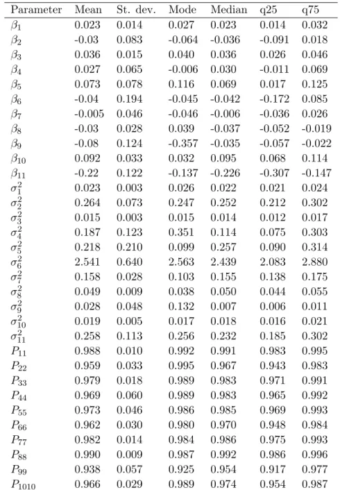
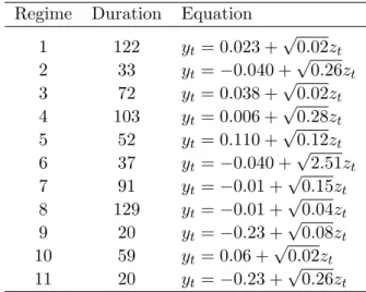
The posterior means, standard deviations, and modes for 11 regimes are reported in Table 6. The regime changes seem to correspond mainly to changes in the the error term variance. Changes in the mean coefficients of the interest rate changes (βj2, j=1,2,. . . ,11) seem less important as their posterior means are close to 0 except in regimes 3, 10 and 11.
5
Simulation study
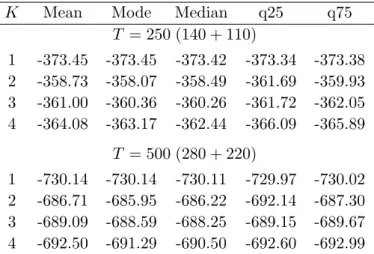
The simulation design is inspired by the empirical results of the previous section. We choose three DGPs, one with a single change point, one with three, and one with seven. In each regime, a sample of size T is generated by an AR(1) process with parameter values and regime durations close to the corresponding estimated results of the previous section. The three DGPs are presented in Tables 7, 10, and 13. For DGPs 1 and 2, 100 repetitions are used, and for the last DGP this number is reduced to 50 because computations are taking a lot of time. A repetition means that a sample of size T is simulated from the DGP and for each sample, the BIC and MLL values are computed for AR(1) models with varying number of regimes. These sets of 100 (or 50) values are then used to produce averages and proportions. 5.1 Single change point (K = 2)
The results of the simulations are contained in Tables 8 and 9. Table 8 contains means (across the 100 repetitions) of BIC and MLL values. Table 9 shows the proportions in which the models with 1, 2 (the true value), 3 or 4 regimes are selected by the BIC or the MLL criterion. From these results, the answers to the two questions we raise in the beginning of 3 are rather clear:
1) The MLL values depend very little on the parameter value chosen for its computation, when the values being considered are the means, mode, medians, 0.25-quantiles (q25), and 0.75-quantiles (q75), where the quantiles are from each marginal distribution. For a given K, the largest difference is 2 (K = 4, T = 500) when comparing mean, mode, and median-based
results (Table 8), which is very small compared to 692. Between mode and median, the differ-ence is always smaller than 1. When comparing mean, mode or median with the quartiles, the differences are a bit larger, with the largest difference occurring for q25 in the cases K = 2,
T = 250 (difference of 3.622) and 500 (difference of 6.19). The sensitivity does not seem to
be related to the sample size T and may be slightly more pronounced for K = 4 than for smaller values. This is expected as inference for an over-parameterized model is likely to be less precise.
2) Concerning the model selection criteria (Table 9), the performance of the BIC in the selection of the correct model is very good (at least 97 per cent of correct choices) and even slightly better than for the MLL. The MLL performance is the best when its computation is based on central values of the parameters (more than 90 per cent of correct choices). When T is increased from 250 to 500, the performance of the BIC and MLL computed with the mode and median increases.
5.2 Three change points (K = 4)
The results of the simulations are contained in Tables 11 and 12. Table 11 contains means (across the 100 repetitions) of BIC and MLL values. Table 12 shows the proportions in which the models with 2 to 6 regimes are selected by the BIC or the MLL criterion. From these results, the answers to the questions raised are rather clear:
1) The MLL values depend very little on the parameter values chosen for its computation. For a given K, the largest difference is 3.95 (for K = 3) when comparing mean, mode, and median-based results (Table 11), which is very small compared to 913. Between mode and me-dian, the difference is smaller than 1 except for K = 3, where the value at the mode is slightly different. When comparing mean, mode or median with the quartiles, the differences are in-creasing with K, because inference for an over-parameterized model is likely to be less precise. 2) Concerning the model selection criteria (Table 12), the performance of the BIC and the MLL criterion (whatever the evaluation point) is good, since the right model (4 regimes) is picked in about 89 to 94 per cent of the repetitions. The risk of choosing a wrong number of regimes is entirely concentrated on the over-parameterized models (especially the model with 5 regimes).
5.3 Ten change points (K = 11)
The results of the simulations are contained in Tables 14 and 15. Table 14 contains means (across the 50 repetitions) of BIC and MLL values. Table 15 shows the proportions in which the models with 9 up to 13 regimes are selected by the BIC or the MLL criterion. From these results, the answers to the questions we are interested in are rather clear:
1) The MLL values (Table 14) do not depend much on the parameter value chosen for its computation, but they vary more than in the two previous cases. The largest difference oc-curs for K = 13 between mean and mode (difference of the order of 10 per cent). However, between mode and median, the differences are very small.
2) Concerning the model selection criteria (Table 15), the performance is not good. The BIC selects the correct number of breaks only in 24 per cent of the repetitions and puts too much weight (50 per cent) on over-parameterized models (K = 12 and 13). This is even much more pronounced with the MLL criterion, since it selects the models with too many regimes in 90 per cent of the repetitions. This bad performance of the criteria may be explained by the following feature of the DGP: there are many regimes, among which some with few observations, and some which are not very different. This confirms our intuition, based on the applications to real data, that there is a tendency to select too many breaks with the type of model we consider.
6
Conclusion
There are two objectives in this paper. The first is to assess the sensitivity of the marginal likelihood value obtained by Chibs’ method in the case of a change-point regression model. The second objective is to compare the model choices resulting from the application of the BIC and of the marginal likelihood criterion. Our findings are firstly that the value of the marginal likelihood computed by Chib’s algorithm is reliable for the class of Markov-switching autore-gressive models. Secondly that the MLL criterion and BIC provide a good performance in choosing the right model, with a marginally better performance of the BIC, except apparently in the case where the number of regimes is large and difficult to identify.
References
Bauwens, L., M. Lubrano, and J. Richard (1999): Bayesian Inference in Dynamic
Econometric Models. Oxford University Press, Oxford.
Chib, S. (1995): “Marginal likelihood from the Gibbs output,” Journal of the American
Statistical Association, 90, 1313–1321.
(1996): “Calculating posterior distributions and modal estimates in Markov mixture models,” Journal of Econometrics, 75, 79–97.
(1998): “Estimation and comparison of multiple change-point models,” Journal of
Econometrics, 86, 221–241.
Elerian, O., S. Chib, and N. Shephard (2001): “Likelihood inference for discretely observed nonlinear diffusions,” Econometrica, 69(4), 959–993.
Fruhwirth-Schnatter, S., and H. Wagner (2008): “Marginal likelihoods for non-Gaussian models using auxiliary mixture sampling,” Computational Statistics & Data
Anal-ysis, 52(10), 4608–4624.
Gelfand, A., and D. Dey (1994): “Bayesian model choice: Asymptotics and exact calcu-lations,” Journal of the Royal Statistical Society B, 56, 501–514.
Hamilton, J. (1989): “A New Approach to the Economic Analysis of Nonstationary Time Series and the Business Cycle,” Econometrica, 57, 357–384.
Johnson, L. D.,andG. Sakoulis (2008): “Maximizing equity market sector predictability in a Bayesian time-varying parameter model,” Computational Statistics & Data Analysis, 52(6), 3083–3106.
Kass, R., and A. Raftery (1995): “Bayes Factors,” Journal of the American Statistical
Association, 90, 773–795.
Kim, C., J. Morley,andC. Nelson (2005): “The structural break in the equity premium,”
Kim, C., and C. Nelson (1999): “Has the US economy become more stable? A Bayesian approach based on a Markov-switching model of the business cycle,” Review of Economics
and Statistics, 81(4), 608–616.
Kim, C.,andJ. Piger (2002): “Common stochastic trends, common cycles, and asymmetry in economic fluctuations,” Journal of Monetary Economics, 49(6), 1189–1211.
Liu, C., and J. M. Maheu (2008): “Are there structural breaks in realized volatility?,”
Journal of Financial Econometrics, 6(3), 326–360.
Maheu, J. M., and S. Gordon (2008): “Learning, forecasting and structural breaks,”
Journal of Applied Econometrics, 23(5), 553–583.
Nakajima, J., and Y. Omori (2009): “Leverage, heavy-tails and correlated jumps in stochastic volatility models,” Computational Statistics & Data Analysis, 53(6, Sp. Iss. SI), 2335–2353.
Newton, M., and A. Raftery (1994): “Approximate Bayesian inference by he weighted likelihood bootstrap,” Journal of the Royal Statistical Society B, 56, 3–48.
Paroli, R., and L. Spezia (2008): “Bayesian inference in non-homogeneous Markov mix-tures of periodic autoregressions with state-dependent exogenous variables,” Computational
Statistics & Data Analysis, 52(5), 2311–2330.
Pastor, L.,andR. F. Stambaugh (2001): “The Equity Premium and Structural Breaks,”
Journal of Finance, 56, 1207–1239.
Pesaran, M. H., D. Pettenuzzo,andA. Timmermann (2006): “Forecasting Time Series Subject to Multiple Structural Breaks,” Review of Economic Studies, 73, 1057–1084. Stock, J. H.,and M. W. Watson (1996): “Evidence on Structural Instability in
Table 1: BIC and MLL of AR(1) models (US GDP growth rate)
K BIC MLL mean MLL mode MLL median MLL q25 MLL q75 1 -336.44 -349.03 -349.06 -349.03 -348.96 -349.01 2 -321.04 -332.66 -332.39 -332.66 -333.62 -333.88 3 -322.02 -334.98 -333.37 -334.68 -335.78 -336.86 BIC: Bayesian information criterion. MLL: marginal log-likelihood, computed by
formula (26) using different parameter posterior values: mean, mode, median, 0.25-quantile (q25) and 0.75 quantile (q75).
Table 2: Posterior results for 1-change point AR(1) model (US GDP growth rate) Parameter Mean St. dev. Mode Median q25 q75
β11 0.576 0.420 0.592 0.580 0.491 0.672 β12 0.345 0.313 0.334 0.336 0.276 0.396 β21 0.478 0.369 0.554 0.481 0.404 0.558 β22 0.333 0.409 0.246 0.330 0.242 0.417 σ2 1 1.471 2.889 1.381 1.282 1.178 1.398 σ22 0.344 0.779 0.261 0.278 0.252 0.313 p11 0.985 0.053 0.993 0.991 0.986 0.996
Table 3: BIC and MLL of AR(1) models (US industrial production growth rate)
K BIC MLL mean MLL mode MLL median MLL q25 MLL q75 1 -927.28 -945.11 -945.13 -945.11 -944.91 -944.94 2 -885.37 -894.61 -894.35 -894.60 -894.90 -894.79 3 -869.70 -882.18 -882.39 -882.16 -882.96 -882.72 4 -855.70 -859.11 -859.35 -859.13 -859.93 -859.67 5 -859.79 -861.68 -858.98 -862.22 -861.35 -863.64 6 -864.41 -864.02 -862.44 -861.88 -867.37 -865.45 7 -872.63 -865.63 -859.97 -864.84 -883.67 -869.86 See Table 1 for explanations.
Table 4: Posterior results for 3-change point AR(1) model (US industrial production growth rate)
Parameter Mean St. dev. Mode Median q25 q75
β11 0.195 0.157 0.307 0.199 0.103 0.291 β12 0.470 0.093 0.441 0.470 0.415 0.526 β21 0.171 0.057 0.200 0.170 0.136 0.207 β22 0.405 0.062 0.395 0.405 0.368 0.443 β31 0.191 0.034 0.171 0.191 0.168 0.213 β32 0.100 0.067 0.144 0.099 0.059 0.139 β41 -0.200 0.520 -0.036 -0.189 -0.523 0.129 β42 0.184 0.354 0.463 0.179 -0.045 0.400 σ2 1 2.075 0.364 2.065 2.043 1.868 2.240 σ2 2 0.680 0.066 0.668 0.678 0.639 0.717 σ2 3 0.262 0.025 0.283 0.260 0.246 0.275 σ2 4 5.390 4.174 4.857 4.259 2.993 6.523 p11 0.988 0.011 0.996 0.991 0.984 0.995 p22 0.995 0.004 0.998 0.996 0.993 0.998 p33 0.995 0.004 0.999 0.996 0.993 0.998
Table 5: BIC and MLL of AR(0) models (US T-bill rate)
K BIC MLL mean MLL mode MLL median MLL q25 MLL q75 1 -512.41 -523.48 -523.48 -523.52 -523.49 -523.49 2 -425.85 -494.43 -438.59 -452.81 -531.50 -527.74 3 -295.82 -307.67 -307.61 -307.67 -308.12 -307.96 4 -269.43 -280.02 -280.08 -280.02 -280.29 -280.32 5 -253.42 -263.06 -263.11 -263.02 -263.53 -263.63 6 -229.82 -235.82 -235.93 -235.86 -236.31 -236.34 7 -226.00 -229.10 -229.47 -229.14 -229.70 -229.76 8 -215.08 -214.96 -215.20 -215.02 -215.56 -215.63 9 -211.38 -208.81 -209.40 -208.90 -209.72 -209.90 10 -212.86 -223.06 -207.33 -210.18 -224.07 -262.45 11 -209.98 -207.65 -198.02 -197.58 -199.03 -208.86 12 -219.39 -213.93 -199.20 -201.70 -221.98 -241.31 See Table 1 for explanations.
Table 6: Posterior results for 10-change point AR(0) model (US T-bill rate) Parameter Mean St. dev. Mode Median q25 q75
β1 0.023 0.014 0.027 0.023 0.014 0.032 β2 -0.03 0.083 -0.064 -0.036 -0.091 0.018 β3 0.036 0.015 0.040 0.036 0.026 0.046 β4 0.027 0.065 -0.006 0.030 -0.011 0.069 β5 0.073 0.078 0.116 0.069 0.017 0.125 β6 -0.04 0.194 -0.045 -0.042 -0.172 0.085 β7 -0.005 0.046 -0.046 -0.006 -0.036 0.026 β8 -0.03 0.028 0.039 -0.037 -0.052 -0.019 β9 -0.08 0.124 -0.357 -0.035 -0.057 -0.022 β10 0.092 0.033 0.032 0.095 0.068 0.114 β11 -0.22 0.122 -0.137 -0.226 -0.307 -0.147 σ2 1 0.023 0.003 0.026 0.022 0.021 0.024 σ2 2 0.264 0.073 0.247 0.252 0.212 0.302 σ2 3 0.015 0.003 0.015 0.014 0.012 0.017 σ2 4 0.187 0.123 0.351 0.114 0.075 0.303 σ2 5 0.218 0.210 0.099 0.257 0.090 0.314 σ2 6 2.541 0.640 2.563 2.439 2.083 2.880 σ2 7 0.158 0.028 0.103 0.155 0.138 0.175 σ82 0.049 0.009 0.038 0.050 0.044 0.055 σ2 9 0.028 0.048 0.132 0.007 0.006 0.011 σ2 10 0.019 0.005 0.017 0.018 0.016 0.021 σ112 0.258 0.113 0.256 0.232 0.185 0.302 P11 0.988 0.010 0.992 0.991 0.983 0.995 P22 0.959 0.033 0.995 0.967 0.943 0.983 P33 0.979 0.018 0.989 0.983 0.971 0.991 P44 0.969 0.060 0.989 0.983 0.965 0.992 P55 0.973 0.046 0.986 0.985 0.969 0.993 P66 0.962 0.030 0.980 0.970 0.948 0.984 P77 0.982 0.014 0.984 0.986 0.975 0.993 P88 0.990 0.009 0.987 0.992 0.986 0.996 P99 0.938 0.057 0.925 0.954 0.917 0.977 P1010 0.966 0.029 0.989 0.974 0.954 0.987
Table 7: DGP with 1 change point
Regime Duration Equation
1 140 yt= 0.60 + 0.35yt−1+ √ 1.50zt 2 110 yt= 0.45 + 0.30yt−1+ √ 0.35zt
Table 8: MLL evaluated in different points for DGP with 1 change point
K Mean Mode Median q25 q75
T = 250 (140 + 110) 1 -373.45 -373.45 -373.42 -373.34 -373.38 2 -358.73 -358.07 -358.49 -361.69 -359.93 3 -361.00 -360.36 -360.26 -361.72 -362.05 4 -364.08 -363.17 -362.44 -366.09 -365.89 T = 500 (280 + 220) 1 -730.14 -730.14 -730.11 -729.97 -730.02 2 -686.71 -685.95 -686.22 -692.14 -687.30 3 -689.09 -688.59 -688.25 -689.15 -689.67 4 -692.50 -691.29 -690.50 -692.60 -692.99 Reported MLL values are means computed from 100 replica-tions. In each replication, T observations are simulated from the DGP defined in Table 7.
Table 9: Model selection performance for DGP with 1 change point
K BIC Mean Mode Median q25 q75
T = 250 1 0.01 0.01 0.01 0.01 0.02 0.02 2 0.97 0.95 0.91 0.95 0.72 0.91 3 0.02 0.04 0.08 0.04 0.26 0.07 4 0.00 0.00 0.00 0.00 0.00 0.00 T = 500 1 0.00 0.00 0.00 0.00 0.00 0.00 2 1.00 0.93 0.96 0.98 0.79 0.90 3 0.00 0.07 0.04 0.02 0.21 0.10 4 0.00 0.00 0.00 0.00 0.00 0.00 Proportions based on same replications as for Table 8.
Table 10: DGP with 3 change points
Regime Duration Equation
1 123 yt= 0.20 + 0.47yt−1+ √ 2.10zt 2 285 yt= 0.17 + 0.40yt−1+ √ 0.68zt 3 293 yt= 0.19 + 0.10yt−1+ √ 0.26zt 4 16 yt= −0.2 + 0.18yt−1+ √ 5.39zt
ztsimulated from N (0, 1) distribution.
Table 11: MLL evaluated in different points for DGP with 3 change points
K Mean Mode Median q25 q75
2 -937.32 -937.18 -937.32 -937.66 -937.58 3 -913.62 -909.67 -912.69 -916.82 -915.14 4 -878.51 -878.21 -878.41 -882.22 -879.36 5 -882.55 -879.71 -879.81 -886.76 -882.79 6 -885.43 -881.90 -881.93 -892.35 -887.00 Reported MLL values are means computed from 100 repli-cations. In each replication, 707 observations are simulated from the DGP defined in Table 10.
Table 12: Model selection performance for DGP with 3 change points
K BIC Mean Mode Median q25 q75 2 0.00 0.00 0.00 0.00 0.00 0.00 3 0.00 0.00 0.00 0.00 0.00 0.00 4 0.91 0.94 0.89 0.96 0.91 0.94 5 0.09 0.06 0.10 0.04 0.08 0.05 6 0.00 0.00 0.01 0.00 0.01 0.01 Proportions based on same replications as for Table 11.
Table 13: DGP with 10 change points Regime Duration Equation
1 122 yt= 0.023 + √ 0.02zt 2 33 yt= −0.040 + √ 0.26zt 3 72 yt= 0.038 + √ 0.02zt 4 103 yt= 0.006 + √ 0.28zt 5 52 yt= 0.110 + √ 0.12zt 6 37 yt= −0.040 + √ 2.51zt 7 91 yt= −0.01 + √ 0.15zt 8 129 yt= −0.01 +√0.04zt 9 20 yt= −0.23 + √ 0.08zt 10 59 yt= 0.06 + √ 0.02zt 11 20 yt= −0.23 +√0.26zt
ztsimulated from N (0, 1) distribution.
Table 14: MLL evaluated in different points for DGP with 10 change points
K Mean Mode Median q25 q75
9 -210.70 -210.76 -210.39 -211.47 -212.44 10 -209.56 -207.17 -207.75 -211.77 -215.59 11 -207.55 -202.33 -202.71 -207.12 -213.84 12 -206.81 -198.47 -199.45 -204.46 -210.51 13 -205.84 -193.95 -194.22 -199.76 -207.00 Reported MLL values are means computed from 50 repli-cations. In each replication, 736 observations are simulated from the DGP defined in Table 13.
Table 15: Model selection performance for DGP with 10 change points
K BIC Mean Mode Median q25 q75 9 0.12 0.00 0.00 0.00 0.00 0.00 10 0.16 0.04 0.00 0.00 0.04 0.04 11 0.24 0.08 0.00 0.04 0.04 0.04 12 0.20 0.16 0.20 0.12 0.20 0.20 13 0.28 0.72 0.80 0.84 0.72 0.72 Proportions based on same replications as for Table 14.
1950 1955 1960 1965 1970 1975 1980 1985 1990 1995 2000 2005 1950 1955 1960 1965 1970 1975 1980 1985 1990 1995 2000 2005 −0.02 −0.01 0.00 0.01 0.02 0.03 0.04 July 1983
1950 1955 1960 1965 1970 1975 1980 1985 1990 1995 2000 2005 −0.04 −0.02 0.00 0.02 0.04 0.06 1 2 3 4 4/60 1/84 6/08
Figure 2: U.S. Industrial production growth rate. Sample period: January 1950-January 2009 (707 observations)
0 50 100 150 200 250 300 350 400 450 500 550 600 650 700 −4 −3 −2 −1 0 1 2 3 6 5 4 3 2 1 7 8 9 10 11 9/57 5/60 6/66 12/69 8/79 8/82 5/89 10/01 2/04 6/07
Figure 3: Three month U.S. T-bill rate change. Sample period: July 1947-September 2008 (735 observations)