Université de Montréal
Quantum Pseudo-Telepathy Games
Aune Lise Broadbent
Département d’informatiqlle et de recherche opérationnelle faculté des arts et des sciences
Mémoire présenté à la faculté des études supérieures en vue de l’obtention du grade de Maître ès sciences (M.Sc.)
en informatique
avril, 2004
\\
07 OCT
cl
\}
.c
dl1
de Montré al
Direction des bibliothèques
AVIS
L’auteur a autorisé l’Université de Montréal à reproduire et diffuser, en totalité ou en partie, par quelque moyen que ce soit et sur quelque support que ce soit, et exclusivement à des fins non lucratives d’enseignement et de recherche, des copies de ce mémoire ou de cette thèse.
L’auteur et les coauteurs le cas échéant conservent la propriété du droit d’auteur et des droits moraux qui protègent ce document. Ni la thèse ou le mémoire, ni des extraits substantiels de ce document, ne doivent être imprimés ou autrement reproduits sans l’autorisation de l’auteur.
Afin de se conformer à la Loi canadienne sut la protection des renseignements personnels, quelques formulaires secondaires, coordonnées ou signatures intégrées au texte ont pu être enlevés de ce document. Bien que cela ait pu affecter la pagination, il n’y a aucun contenu manquant.
NOTICE
The author of this thesis or dissertation has granted a nonexclusive license allowing Université de Montréal to reproduce and publish the document, in part or in whole, and in any format, solely for noncommercial educational and research purposes.
The author and co-authors if applicable retain copyright ownership and moral rights in this document. Neither the whole thesis or dissertation, flot substantial extracts from it, may be printed or otherwise reproduced without the author’s permission.
In compliance with the Canadian Privacy Act some supporting forms, contact information or signatures may have been removed from the document. While this may affect the document page count, it does flot represent any loss of content from the document.
faculté des études supérieures
Ce mémoire intitulé:
Quantum Pseudo-Telepathy Games
présenté par: Aune Lise Broadbent
a été évalué par un jury composé des personnes suivantes: Michel Boyer président-rapporteur Alain Tapp directeur de recherche Gilles Brassard codirecteur Stefan Wolf membre du jury Mémoire accepté le
Le traitement de l’information quantique est au confluent des sciences physique, mathématiques et informatique; il vise à déterminier ce qu’on peut et e peut pas faire avec l’information quantique. Le sujet de ce mémoire est la complexité de la communication, qui est un domaine de l’informatique qui vise la quantification de la communication nécessaire à la résolution de problèmes distribués.
La pseudo-télépathie est une application surprenante du traitement de l’infor mation quantique à la complexité de la communication. Grâce à une ressource quantique appelée « intrication », deux joueurs ou plus peuvent accomplir une tâche sans comrnnnïqner, tandis que ceci serait impossible pour des joueurs clas siques (qui n’ont pas accès à l’intrication). Un jeu de pseudo-télépathie à n joueurs se présente comme suit: chaque joueur reçoit en entrée une question. Sans com muniquer, chacun émet en sortie une réponse. Le jeu est gagné si les réponses conjointes satisfont une certaine condition. Il s’agit d’un jeu de pseudo-télépathie si les joueurs quantiques peuvent gagner de façon systématiqile, tandis que ceci est impossible pour les joueurs classiques.
Dans ce mémoire, nous décrivons sept jeux de pseudo-télépathie, tirés de la littérature de la physique et de l’informatique quantique. Nous incluons aussi des résultats originaux de l’auteur. Les jeux sont présentés du point de vue informa tique, et de façon uniforme, ce qui facilite leur comparaison. Certains points de comparaison sont: le nombre de joueurs, la taille de l’entrée, la taille de la sortie, la condition gagnante, l’état intriqué partagé et la probabilité maximale de réussite pour les joueurs classiques.
Mots clés: informatique quantique, complexité de la communication quantique, non-localité, intrication, théorème de Beil, échappatoire de la détection.
Quantum information processing is at the crossroads of physics, mathematics and computer science; it is concerned with what we can and cannot do with quantum information. This thesis deals with communication cornplexfty, which is an area of computer science that aims at quantifying the amount of communication necessary to solve distributed problems.
Pseudo-telepathy is a surprising application of quantum information processing to communication complexity. Thanks to a quantum resource called “entangle ment”, two or more quantum players can accomplish a task with no communica tion. whereas this would be impossible for classical players (who do not have access to entanglement). A pseudo-telepathy game with n players is the following: each player receives as input a question. Without communicating, each player outputs an answer. The players win if their joint answers satisfy a certain condition. \‘Ve say that the game exhibits pseudo-telepat.hy if quantum players can svstematically succeed at this game, whereas this woiild be impossible for classical players.
In this thesis, we describe seven pseudo-telepathy games which appear in the physics and quantum information processing literature. We have also included original resuits of the author. The games are presented frohi a computer scientist’s perspective, and in a uniform way, in order to facilitate comparison. Some points of comparison are: number of players, size of the inputs, size of outputs, winning condition, shared entangled state and maximum success probability for classical players.
Keywords: quantum information processing, quantum communica tion complexity, nonlocality, entanglement, Beil’ s theorem, detection loophole.
CONTENTS RÉSUMÉ . iII iv viii xi xii xiii xiv XV xvi ABSTRACT CONTENTS LIST 0F TABLES LIST 0F FIGURES LIST 0F APPENDICES LIST 0F ABBREVIATIONS NOTATION DEDICATION ACKNOWLEDGEMENTS PREFACE CHAPTER 1: INTRODUCTION
1.1 Measurements and Spooky Action at a Distance 1.2 Bell’s Response
1.3 Pseudo-Teïepathy
1.3.1 Telepathy alld Pseudo-Telepathy . .
1.3.2 Pseudo-Telepathy and Bell’s Theorem 1.4 Related Work
1.5 Contributions
vi
2.1 The Qubit
Complex Tuner Product Space Basic Operations
n-Qubit Systems
Operations on Parts of a System Entanglement
CHAPTER 3: PSEUDO-TELEPATHY
3.1 Playing the Games 3.2 $trategies
3.2.1 The Promise
3.3 Physical Realizatiolls and Loopholes 3.3.1 Noisy Detectors
3.3.2 Inefficient Detectors 3.4 Presentation of the Games
CHAPTER 4: TWO-PARTY GAMES
4.1 The Impossible Colouring Game 4.1.1 A Quantum Winning Strategy 4.1.2 Classical Success Proportion 4.1.3 Special Case of the Impossible 4.2 The Distributed Deutsch-Jozsa Game 4.2.1 A Quantum Winning Strategy 4.2.2 Classical Success Proportion 4.3 The Magic Square Game
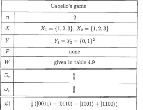
4.3.1 A Quantum Wirining $trategy 4.3.2 Classical Success Proportion 4.4 Cabello’s Game
4.4.1 A Quantum Winning Strategy 4.4.2 Classical Sllccess Proportion
28
Game 33
33
3$ 39
CHAPTER 2: QUANTUM INFORMATION PROCESSING
2.2 2.3 2.4 2.5 2.6 8 8 9 9 11 12 13 15 15 17 20 22 25 25 26 Colouring
4.5 The Magie Square and Cabello’s Games Are Equivalent . 44
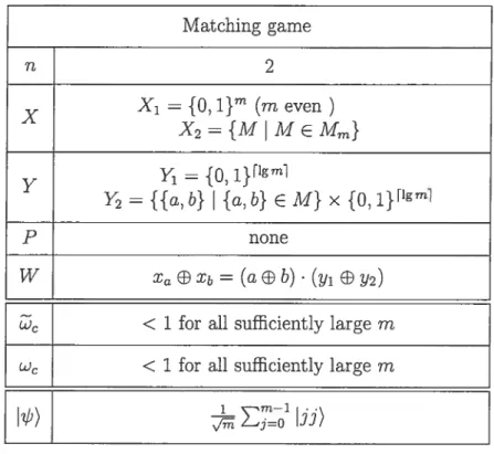
4.6 The Matching Game 49
4.6.1 A Quantum Winning $trategy . . . 50
4.6.2 The Hidden Matching Problem . 52
4.6.3 Classical Success Proportion 52
CHAPTER 5: MULTI-PARTY GAMES 54
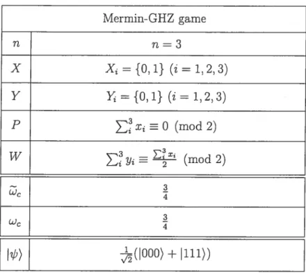
5.1 The Mermin-GHZ Three-Party Game 54
5.1.1 A Quantum Winning Strategy 55
5.1.2 Classical Success Proportion 57
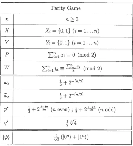
5.2 The Parity Game 59
5.2.1 A Quantum Winning Strategy 59
5.2.2 Classical Success Proportion 61
5.2.3 Classical Success Probability 75
5.2.4 Towards Closing the Detection Loophole 87
5.3 The Extended Parity Game 94
5.3.1 A Quantum Winning Strategy 95
5.3.2 Classical Success Proportion 96
5.3.3 Towards Closing the Detection Loophole 97
CHAPTER 6: CONCLUSION 101
6.1 Future Work 105
3.1 Presentation of the games 27 4.1 31 4.2 33 4.3 35 4.4 39 4.5 40 4.6 42 4.7 42 4.8 43 4.9 . . . . 43 4.10 . . . 49 4.11 50 5.1 55 5.2 60 5.3 66 5.4 74 5.5 75 5.6 81 5.7 82 5.8 84 5.9 84 5.10 85 5.11 95 102 103 and Cabello’s game
Impossible colouring game
Impossible colouring game (rn = 3)
Distributed Deutsch-Jozsa game Magic square game
A 3 x 3 array of observables Alice’s strategy
Bob’s strategy Cabello’s game
Winning conditions for Cabello’s game Winning conditions for the magic square Mat ching game
Mermin-GHZ game Parity game
Number of questions that yield a winning answer Values of n/2 + 3n (mod 4) for even n
Optimal strategies
Values of £ (mod 4) for odd n Values of n— 21? (mod 8) for odd n
Values of £ (mod 4) for even n Values of n— 21? (mod 8) for even n
Values of n— 21?3 (mod 8) for even n
Extended parity game
6.1 Two-party games: comparison table part I . . .
Appendix I: Proof of lemma 5.2.5 xvii
BK$ Beil-Kochen-Specker EPR Einstein-Podolsky-Rosen GHZ Greenberger-Horne-Zeilinger
R real numbers C complex numbers
z imaginary number, r =
c complex norm of c
7d d-dimensional complex inner product space
b) quantum state
b) normofb)
Ax) Hamming weight of a binary string x bitwise comple ment of x
modular equivalence, (mod 2) if not specifled lg(x) base-two logarithm, log2(x)
(G) maximum success proportion, over ail possible deterministic strate gies for classical players that play the game G
w(G) maximum success probability, oyez ail possible strategies for classi cal players that play the game G
w(G) maximum success probability, oyez ail possible strategies for quan tum players that play the game G
p probability that a player’s answer corresponds to the predictions of quantum mechanics in a game with errors
p (G) maximum value of p for which a classical strategy can succeed as well as a quantllm strategy
rj probability that a player outputs something other than I in an error-free game
r](G) maximum value of 1] for which a classical strategy can succeed as
I would like to thank mv supervisors. Dr. Gilles Brassard and Dr. Alain iapp for their help, encouragement and support. Thank-you also to my friends and family, in particular, my mother, father, sister, and Didier. Thanks to you, I found the motivation to bring this project to term. I also thank my grad school friends here at the Université de Montréal.
Many thanks to the Natural Sciences and Engineering Research Council of Canada, the Université de Montréal and the National Bank of Canada, for having funded this work.
This research project was motivated by the need for a comprehensive survey of work that lias been clone in the multi-disciplinary area of pseudo-telepathy.
This need became apparent to me when, after Gilles Brassard, Alain Tapp and I published a pseudo-telepathy game that we thoughwas new [BBTO3], Serge Massar kindly pointed out to us that similar work [Mer9Ob] had appeared more than ten years ago in the physics literature.
Since writing this Master’s thesis, I have prepared, along with my co-authors, two manuscripts that originate from tRis work. Quantum Pseudo- Telepathy [BBTO4a] is a survey of pseudo-telepathy games, and Recasting Mermin’s muÏti-pÏayer game into the framework of pseudo-telepathy [BBTO4b] presents the novel resuits from section 5.2 of the present document, some of which have been greatly simplffied.
INTRODUCTION
Niels Bohr, one of the fathers of quantum physics, said that if studying quantum mechanics doesn’t make yôu dizzy, you haven’t understood it properly.
The present thesis, which deals with quantum information processing (QIP), is meant to he a remedy to the sometimes profound dizziness we feel when studying such strange concepts. With the use of pseudo-telepathy games, it objectively shows the power of the quantum world and unveils some of its mysteries.
Q
IP is concerned with what we can and cannot do with quantum information; its fundamentals lie in the area of quantum mechanics which is the study of matter at the atomic level. Quantum mechanics is the best tested theory that describes our world. To better understand the wonders of quantum mechanics and thus of QIP, it is good to see how our predecessors saw and thought about these ideas.1.1 Measurements and Spooky Action at a Distance
According to the predictions of quantum mechanics, when performing measure ments related to the position and momentum of an electron, the precise knowledge of one quantity prevents such a knowledge of the other.
This prompts the following question: If it is impossible to measure both the po sition and momentum of an electron with arbitrary precision, then can an electron have both a position and momentum?
for many physicists. including Bohr, the answer to this question is that the two quantities cannot simultaneously exist. As Jordan asserts:
observations not only disturb what has to be measured, they produce it! ... We compel it [the electron] to assume a definite position . .. we
For Einstein, however, the answer was different. He did not reject the predic tions of quantum mechanics, but was bothered by its consequences. for him, if the quantum theory cannot describe both the position and momentum of an electron, then the quantum theory does not provide a complete description of the electron. Thus, he concluded that quantum mechanics must 5e incomp1ete”.
In support of this conviction, Einstein published in 1935 an article with Podol sky and Rosen [EPR35], in which they present a gedanken experiment. A gedanken (“thought”) experiment is “a hypothetical sequence of events about which the quan tum theory makes quite definite predictions” [Mer9Oa]. The purpose of the scenario is to challenge the quantum theory on the basis of its predictions, and so to make the point, it is not necessary to actually carry out the experiment. This particular gedanken experiment is meant to provide evidence of the existence of elements of reaiity, also called hidden variables, deflned as in [EPR35]:
If, without in any way disturbing a system, we can predict with certainty (i.e., with probability equal to ullity) the value of a physical quantity, then there exists an element of physical reality corresponding to this physical quantity.
In the gedanken experiment, Einstell, Podolsky and Rosen (EPR) consider two particles that may originally interact. They are then separated into two distinct regions, A and B. EPR then daim that by choosing to measure either the position or the momentum of a particle in region A, one could learn either the position or the momentum of a second particle in region B. Since the measurements in A can not disturb the particle in region B, they conclude that the particle in region B must have had both its position and momentum all along, i.e. there are elements of reality that correspond to the position and momentum.
Because the quantum theory cannot assign values to both quantities at once, it must provide an incomplete description of phvsical reality. But there is an alterna tive explanation: the position or momentum iiieasurement at A could influence the the particle at B, setting its position or momentum: “Spukhafte Fernwirkung” or
“spooky action at a distance”. This phenomenon, which is predicted by quantum mechanics, was also rejected by Einstein. Fiedid not doubt the predictive power of
quantum mechanics, but insisted that it was incomplete. According to him, (and supported by his gedanken experiment), there had to be some underlying informa tion (elements of reality or hidden variables) which determines the outcome of the measurements. The elements of reality are not directly observable, yet we witness their effect each time that we perform a measurement in region A or B.
The reaction of other physicists to the EPR paper was that this was an area of meta-physics; the question was unanswerable to scientific observation, and unwor thy of argumentation. As Pauli wrote,
As O. Stem said recently, one should no more rack one’s brain about the problem of whether something one cannot know anything about exïsts all the same, than about the ancient questions of how many angels are able to sit on the point of a needle. But it seems to me that Einstein’s questions are ultimately always of this kind. [EBBZ1]
1.2 Bell’s Response
In 1964, Bell gave a shocking reply to EPR by publishing a paper [Be164] in which lie proposes a gedanken experiment that mules out any possibility of hidden variables in the quantum theory.
Having put the EPR thesis in perspective in the previous section, one should be surprised that Bell was able to irrefutably show lis resuit. EPR’s argument was not a question of meta-physics, after ail! The physicist Henry Stapp called BelÏ’s discovery “the most profound discovery of science” [$taZ5]. Tri order to be able to state Bell’s theorem, we first give some definitions:
Definition 1.2.1. A local theory is one in which no action performed at location
A can have an instantaneous (faster than light) observable effect at location B. Definition 1.2.2. A reatistic theory in one in which ail measurement outcomes pre-exist before the measurement.
With this formalism, we note that EPR argued in 1935 that any complete theory must be local and realistic, Bell’s answer is to show the following theorem: Theorem 1.2.1 (Bell’s Theorem). No tocat. reatistic theory cari explain the predictions of quantum mechanics.
Beil proved his theorem by exhibiting a quantum system involving two parti des. He showed that if we assume the presence of hidden variables, as well as the locality condition, then the outcomes of the experiment are in contradiction with the outcomes predicted by quantum mechanics. Thus quantum mechanics is not a local, realistic theory.
We won’t give the details of Bell’s argument here, because in the next one hundred pages or so of the present document, we will effectively prove over and over again Bell’s theorem. Exactly how this is done is explained in the following
section.
1.3 Pseudo-Telepathy
The previous section presented a part of the history of physics, which motivates our research. We wish to adopt for the rest of this thesis the QIP paradigm; for that, we must note an important correspondence: a classicat theory denotes a tocaÏ
and realistic theory. Thus, if something or someone is constrained to act in a
classical fashion, they do not have access to any quantum mechanical resource. To which quantum mechanical resource are we referring? The answer is entan gtement, the “iron to the classical world’s bronze age” [NCOO]. The properties of this resource are stili not well understood, but we can say for sure that it is thanks to entanglement that we get resuits sucli as Bell’s theorem. Entanglement causes
the “spooky action at a distance” (also referred to as nonlocaÏity) that Einstein rejected. It is also thanks to entanglement that we can devise amazing games such as pseudo-telepathy games: pseudo-tetepathy is defined inforrnally as the charac
players (sharing entanglernent) aiways succeed, but for which the classical players have an unavoidable, non-zero probability of failure.
1.3.1 Telepathy and Pseudo-Telepathy
Telepathy is “communication from one minci to another without using sensory perceptions”. With this definition in minci, what do we mean by psendo-telepathy? Suppose that we have a pseudo-telepathy game that involves two players, Alice and Bob. They are flot allowed to communicate with each other. If they were classical, we know that they would sometimes fail. However, if they share entanglement,
they aiways succeed at the given game. So, if we introduce a witness, who looks
at the results of the game, but who does not believe in the quantum theory (or anything beyond the classical theory), then the only possible explanation, given that Alice and Bob consistently win, is that they must have a way to signal to each other—they must be telepathic!
We know, however, that this is flot the case. We know that Alice and Bob share entanglement and that it is thanks to this that they appear to be telepathic. Hence, pseudo-telepathy. There are limits to what Alice and Bob, who share entanglement, can do. Specifically, “entanglement alone cannot be used to signal information— otherwise faster-than-light communication would be possible and causality would be violated” [BraO3].
1.3.2 Pseudo-Telepathy arid Bell’s Theorem
We’ve alreadv stated that this document is dedicated to proving Bell’s theorem. Indeed, pseudo-telepathy proves Bell’s theorem in the following way: in pseudo telepathy, the quantum players have a clear advantage over the classical players. Recail that classical players are restricted to a local, realistic theory. Since the quantum players aiways win and the classical players do not, we conclude that no local, realistic theory can reproduce the predictions of quantum mechanics—which is precisely the essence of Bell’s theorem.
1.4 Related Work
Research in the area of pseudo-telepathy originally appeared in the physics lit.erature. as these games provide a proof of Bell’s theorem. This area of research is stili active. 0f course, the terrninology, notation and even the context differ widely from the usual paradigrn adopted in QIP, which is part of the challenge in
writing the present dodilment. Pseudo-telepathy games sometimes appear under the following names:
• Bell’s theorem without inequalities [GHSZ9O]
• Bell’s theorem without inequalities and without probabilities [CabOlb] • GHZ-type game
• always-vs-never refutation of Einstein, Podolsky and Rosen [IVIer9Oe] • BeR inequality [BM93]
• ali-versus-nothing violation of local realism [CPZO3]. • “ail versus nothing” inseparability [CabOlb]
• inequality-free proof of Bell’s nonlocality theorem [Ara99]
Other works on pselldo-telepathy appear in the QIP literature, more precisely in a communication comptexity context. Here, we find pseudo-telepathy under such headings as “nonlocality games”, “cooperative games”, “interactive proof systems” and of course, “pseudo-telepathy”. We also find related work in the philosophy literature.
1.5 Contributions
The present thesis is a collection of pseudo-telepathy games. far from being a simple literatiire review, this document presents many original contributions:
1. The fact that the games appear in a variety of contexts (theoretical physics, experimental physics and QIP—see section 1.4) means that a considerable amount of work has been done to make a uniform presentation of the games and reiated resuits.
2. In section 3.2.1 (“The Promise”), we give a formai definition of a promise game.
3. In section 4.5 (“The Magic Square and Cabello’s Game Are Equivalent”), we provide a definition of equivatent two-player games, and show that the two games are equivalent.
4. In section 5.2 (“Parity Game”), theorems 5.2.2 and 5.2.6, concerning the cias sical success proportion and classicai success probability of the parity game are proven. This is original work of the author.
5. Also in section 5.2, theorem 5.2.16, concerning error-free strategies for the parity game is proven. This is also original work of the author.
1.6 Structure of the Thesis
The remainder of the present document is divided into four chapters. Chapter 2 gives the basic notation and priilciplesof QIP. Chapter 3 is concerned with pseudo telepathy in general: we give a formal defiuition of pseudo-telepathy and present general notation and concepts that are useful in presenting pseudo-telepathy games. Finally, chapters 4 and 5 are dedicated to the presentation of a total of seven pseudo-telepathy games (eight if we distinguish the two equivalent games). They are divided into chapter 4, which presents two-party games and chapter 5, which presents muÏti-party games, which are games with three or more players.
QUANTUM INFORMATION PROCESSING
In this chapter, we give definitions and theorems that relate to quantum information processing, which we will need in the rest of the document. This is not meant to be a comprehensive introduction to the area, but oniy to specific tools that are required in the context of pseudo-telepathy. A good reference for quantum information processing is [NCOO].
2.1 The Qubit
The bit is the fundamental unit of classical computation and classical informa tion. Quantum computation and quantum information are built upon an analogous concept, the quantum bit or qubit. Qubits, like bits, are realized on actual physical systems. Here, we treat them as abstract mathematical objects. A qubit can be in the state O) or 1). It can also be in a superposition of states O) and 1): an arbi trary qubit can be written as = e O)+/3i), where c8 C and 2+32 = 1.
We also write
)
as a coÏumn vector using the convention that {O), l)} form the standard basis:[;Ï
The nature of quantum information implies that we cannot extract the ampli tudes o and from b); we are only able to make statistical inferences about these values (more about this in section 2.3). It is also impossible to clone quantum information. That is, it is not possible to start from one qubit in an unknown state and make two identical copies of it.
2.2 Complex Inner Product Space
Let 7t denote a a d-dimensional complex iniler product space (a complex vector space equipped with a complex iniler product) over C. The notation 7 rerninds
115 0f a HiÏbert space; this is because the finite dimensional complex inner product
spaces that corne up in quantum computation and quantum iuforrnation are Hilbert spaces. Qubits are column-vectors in K2. We define
(
(“bra”) to be the row vector that is the conjugate transpose of b) (“ket”). Then (i), usually written as (‘çb), denotes the muer product of ç) with b). The norm of ‘), denotedH)H
is defined as = Thus qubits have norm 1.2.3 Basic Operations
We introduce three basic operatiolls on qubits: initialization, unitary transfor mation and measurement. In what follows, we take for granted that these opera tions eau be performed perfectly.
1. Initialization. It is possible to initialize a qubit to the state O) or 1).
2. Unitary Transformation. We can perforrn any unitary transformation, given by
U= 1101
1111
where u C. U is unitary if and only if UU = I, where U is the conjugate
transpose of U and I is the identity rnatrix. We also denote the above U as:
U
O) i,’ uooO) +n1)
U
A very useful unitary transformation is the Hadamard transform, given by
1 1 1
1—1•
In other words,
0) 0)+1))
3. Measurement. So far, we’ve seen that we can initialize a qubit and perform unitary transformation. We also need to have awayto measure a. qubit. As we have already stated, a measurernent will flot yield the complete description of the qubit; measurement in the standard basis of an arbitrary qubit o0)+j31)
resuits in the following:
O with probability 2
0)+1) ‘S
11
with probability 2Furthermore, measurement alters the qubit. After the measurement, the state cottapses to 0) if O was measured and 1) if 1 was measured.
It is also possible to measure an arbitrary qubit b) with respect to any orthonormal basis B of 72, say B = {b1), b2)}. Then the probability of
getting resuit b when measuring
)
is given byp(b =
Given that resuit b was rneasured, the state of the quantum system immedi
ately after the measurement collapses to b).
Wliat if we want to start a protocol in a state other than O) or 1), for example,
formation (for the specific example, we would apply the Hadamard transform). Hereafter, if we start a protocol in a state
)
other than O) or 1), it is because, implicitly, we have applied a unitary transformation to one of the basis states to obtain).
2.4 n-Qubit Systems
We have seen how we can work with a single qubit. Now, we would like to be able to work with a system of n qubits. It turns out that we can easily extend the basic operations on a single qubit to operations on any number ofqubits.
An n-dimensional qubit system is a 2-dimensiona1 norm 1 vector in for example, for n = 3, an arbitrary 3-qubit quantum register can 5e written as:
cr000 c010 O11 ax) 0ioi where = 1
Formally, we combine systems with the Kronecker product (also erroneously calÏed the tensor product) ofvectors; if b) = O) +1) and
)
= ‘O) +ff1),then b) ®
) e
72 ® 2 = 722, ando? cç
if
73cVIn this representation, t.erms like a denote the 2 x 1 submatrix whose entries are proportional to ), with overail proportionalitv constant c. When using the ket notation, we often drop the symbol. Thus, 0) ® 0) = 0)0) = 00).
The same three basic operations of section 2.3 hold for an n-qubit system: we may initialize to any basis state x) where x
e
{0,l}n.
We can perform any unitary operation given by a 2 x 2’ unitary matrix U. We can perform a measurement of a state?/)
in any orthonormal basis B of ?-t2, say B = {b1),..., b2n)}. Theprobability of getting resuit b when measuring b) is given by:
p(b) =
Given that resuit b was measured, the state of the quantum system immediately after the measurement collapses to b).
When referring an n-qubit system, we use denote‘ ® U ® 0
U
by U®hl. We also wnte On) to represent 00. . . 0). Also, as in the one qubit case, if we start aprotocol in a state ‘) other than a basis state, it is because, implicitly. we have applied a unitary transformation to one of the basis states to obtain b).
2.5 Operations on Parts of a System
$o far, we’ve considered operations on a system as a whole. It is also possible to act on part of a system.
for example, Alice and Bob can share a two-qubit system: Alice takes the first qubit and Bob the second. Once this is done, they may become physically separated. $ay Bob applies a unitary transformation U. Then the effect on the system is to apply the transformation I O U, given by the matrix:
‘u00 UO1 O O
‘u10 Uii O O
I®U=
O O tc00 U01
o o ‘u10 Ui;
This can be generalized to an operation on any partial system of any dimen sion. Ivleasurements may also 5e performed on part of a system: for any state
b) E ?1ABC, we can measure the subspace 3. A partidillar state of interest is:
=
By measuring the subspace B, we obtain the resut i with probability 2
and the resulting state is a)i)c).
It is useful to note that we get the same effect if we perform two measure ments on different subsystems, or if we perform the measurements together. Also, the same effect is obtained if two parties are to perform some unitary transforma tion and then measure—regardless of the order in which the parties perform their actions.
2.6 Entanglement
Given an m ± n qubit state ‘) E 7m0 we say that J) iS a pTOdUCt state if b) = ‘y)6) for y) E 712m and i) E 2u. If b) is not a product state, then h is
an entangled state.
Examples of entangled states are the BeÏt states:
(OO) + 11))
= — 11))
= (IO1) + 10))
1
The state Irj is also known as an Einstein-Podolsky-Rosen (EPR) pair. We will use it to demonstrate one of the “mysteries” of entanglement: If Alice and Bob share an EPR pair. and Alice measures her qubit in the standard basis the outcome will be O with probability and 1 with probability . Likewise. Bob’s
measurement in the standard basis will yield O with probability and 1 with probability . However, we know for sure that AÏice and Bob’s outcomes will 5e
opposites. Hence, by knowing one of the outcomes, we can predict with certainty the other; this “spooky action at a distance” is a surprising feature of entanglement. Furthermore, if Alice and Bob perform measurements of ‘I’j, in any basis, we can be sure that the outcomes will be opposites.
We will make use of the state
)
in the following context: Suppose Alice and Bob share two I) states:= (OO) + 11)) ® (OO) + 11)),
where Alice lias the flrst and third qubits. and Bob the second and fourth ories. ‘Ne cari re-write this as:
= (OOOO) + 0101) + lolo) + 1111))
where, this time, Alice lias the first two qubits and Bob the second two. Gener alizing this, we see that if Alice and Bob share n cIj states, then they share the entangled state )®n
=
(
PSEUDO-TELEPATHY
The goal of this chapter is to facilitate discussion by presenting notation and resuits that relate to pseudo-telepathy games in general. At the end of the chapter, we give details on the presentation of the garnes. The general framework of this chapter is useful in chapters 4 and 5, where several games are presented.
3.1 Playing the Games
Definition 3.1.1. An n-player garne G = (X, Y, P, W) consists of:
• X = X1 x X2 x ... x X,2, where X1, X2,. . . X are sets of possible inputs
• Y = Y1 x Y2 x ... X Y, where Y1, Y2,. . Y are sets of possible outputs
• a predicate P on X called the ponise
• a relation 117 on X x Y, called the winning condition
An instance (figure 3.1) of the game proceeds in the following way:
1. A question x = X1,x2,. . . ,x E X is chosen from the set P. (We use a slight abuse of notation, using P as a predicate and as the set of elements in X that satisfy the predicate)
2. Each player i receives his input x E X.
3. Each player i responds with an output yj
e
Let ,‘ = Y1,Y2,• .. ,y be the answer.
4. The players win if (x, y) W, and they lose otherwise. The following rule governs the way the game is played:
step 1:
step 2:
x is chosen from the set P 1etx=x1,x2,...x
player i produces output y. 1ety=y1,y2,...y
P
xi
player i receives input x.
X2 X??, < Yi < Y2 y?? 1 2 n 1 2 n step 3: step
4:
yes noNo communication between the players is allowed during the game. Before the start of the game, the players may agree on a strategy. They
may share random bits, and, if they are quantum players, they may share entanglement.
Suppose that we have a game G = (X, Y P, W) such that there exists an
Xo
e
X such that P(0) = true and x0Ø
domain(W). Then there is no way ofwinning if the players are given question XO. This Ïeads to a game that is not inter
esting in the context that we wish to study. Hence, ail games G = (X, Y P, W)
that we consider have the property that:
Vx
e
X,P(x) = truce
domain(W). (3.1)3.2 Strategies
Players, whether classical or quantum, will always use a strategy to determine what their answer y will 5e. given a particular question x. According to game theory, a player’s strategy is “a plan which specifies what choices he will make in every possible situation, for every possible actual information which he may possess at that moment . . .“ [NM44].
In the games that we study, as either ail players win or they ail lose, their best strategy is to collaborate to maximize their probability of winning. Such games are in the class of cooperative games. We specify if the players are ctassical or quantum. Classical players may have a deterministic strategy. They may also have access to shared randomness, which allows them to use a pro babitistic strategy, which is a probability distribution over a finite set of deterministic strategies. Quantum play ers have access to entanglement, which they may exploit in their quantum strategy. In pseudo-telepathy, quantum players have a winning strategy and classical players do not. For the classical players, we want to know just how well they can succeed. We say that a strategy is a winning strategy if it succeeds on ail instances of the game. We also classify the success of strategies according to the following:
Definition 3.2.1. A deterministic strategy is successful in pToportzon p if the ratio of the number of instances for which the players win and the total number of instances is p.
Definition 3.2.2. A strategy is successful withpTobabitity q if it wins any instance
with probability at least q.
$ome strategies are better than others; those that are optimat reach the follow
ing optimal bounds:
Definition 3.2.3. Let G be a game. We define:
1. (G) to be the maximum success proportion, over ah possible deterministic strategies, for classical players that play the game G
2. w(G) to be the maximum success probabihity, over all possible strategies, for classical players that play the game G
3. Wq(Gn) to be the maximum success probabihity, over all possible strategies, for quantum players that play the game G
In pseudo-telepathy, the quantum players have a winning strategy, and the classical players do not. This amounts to saying that wq(Gn) = 1 and (G) < 1.
Definition 3.2.4. An n-player pseudo-telepathy game is
a game G for which wq(Gn) 1 and (G) < 1
Suppose that a deterministic strategy is successful in proportion p < 1. Then
there is at least one instance of the game where the players systematically fail, hence the strategy’s success probability is q = 0, so we must consider probabihistic
strategies in order to obtain a meaningfuÏ bound on w(G). However, the next two theorems state that if we know that the maximum success proportion of a deterministic strategy is p, then we have that w(G) p.
Proposition 3.2.1. Let G be a game. Then (G) is the maximum pro babitity that the ptayers win if the questions are asked uniformty at random among questions that satisfy the promise.
Proof. We consider a general probabilistic strategy s which is a probability distri bution over a fuite set of deterministic strategies. say {Si, 8m} Let Pr(s)
be the probability that strategy s is chosen, and let p be the success proportion of strategy s. The probability that the players win the game is:
m m
Pr(s)p < ZPr(sj)lc(Gn)
=
furthermore, by defluition, there exists a strategy that succeeds with probabihty E Theorem 3.2.2. For any game O, w(G) <(G).
Proof. Consider any strategy s that is successful with probability By definition, for every question x satisfying the promise P, the probability of winnillg on question x is Pr(win x) > w(G). If the question is chosen uniformly at
random, the probability q of winning the game using the same strategy s is
— Pr(win x) q xEP -xP = w(G)
By proposition 3.2.1, (G) q, and since q > w(G), then (G) w(G7). E
Lemma 3.2.3. Let G = (X, Y P, W) be a game with(G) < 1. Then
w(G)
<
Proof. Since L(G) is the maximum success proportion, over ail possible deter ministic strategies, for classical players that play the game G, it is the ratio of the maximum number of questions that satisfy the promise and on which classical players can win, and the total number of questions that satisfy the promise.
$ince (G) < 1, the next best alternative is that (G) = 171. So we
PH1
conclude that w(G71) < ——. LI
3.2.1 The Promise
In step 1 of an instance of the game G (X, Y, P, W), a question is chosen among ail questions satisfying the promise P. In other words, it is possible that a certain x Œ1,X2,... x E X, yet x is not a valid question (P(x) = fatse).
Although they make the game more artificial, we often (but not always—see sec tions 4.3, 4.4 and 4.6) rely on sucli promises in order to ensure an advantage for the quantum players.
The concept of a promise game lias appeared in QIP literature before, for example, in the context of the Deutsch-Jozsa problem [DJ92]. In the case of pseudo-telepathy, we give our interpretation for defining a game with and with out a promise:
Definition 3.2.5. Let G = (X, Y, P, W) be a game. We say that G is promise
free if ail of the following liold: 1. VxEX,P(x)=true
2. VxEX,yEYsuchthat(x,y)ØW
Otherwise, we say that G is a promise game.
A game is promise-free if ail three conditions of definition 3.2.5 are met. The motivation for the first and second conditions is obvious. The third condition is there to ensure that each element in Y = Y1 x Y2 x ... x Y,-, is useful. In other
words, one cannot introduce a bogus element in one of the player’s answers, and then conclude that the game is error-free according to condition 2.
0f course, given a game G = (X, Y, P, W) where P(xo) is false for a given
Xo é X, it is possible to convertit to a game G = (X, Y P’, W’) where P’(zo) = true
(and P’(x) = P(x) otherwise), by simply specifying in the winning condition
W’ that Vg E Y, (x y) E W’ (and W’ is otherwise unchanged from W). By repeatedly applying this technique to ail such x0, we convert G,., into a game
G = (X, Y, P”, W”) where P” is the constant true predicate, and so we have
eliminated the need for the promise P. Note, however, that according to definition 3.2.5, G is stili a promise game (since, for example, (xo, y)
e
W Vye
Y).We may also proceed in the opposite direction. Given a game G,.,, suppose that x0 E X such that Vy
e
Y, (tx0, y) E W. We can then derive a new game G, = (X, Y, P’, W’) where P’(xo) =f
aise (and P’(x) = P(x) otherwise) andwhere x0 is removed from domain(W), which yields W’1. Continuing in this way, we arrive at a game G = (X, Y P”, W”) such that Vx E X, either P”(x) is false
or ê Y such that (x, y) W”. We cali such a game a min-promise game (since
{x E X P”(x) = true} is smallest possible). In the present document, we will
consider games G,., in their min-promise form only, since by the following lemma,
(G) is smallest for these games.
Lemma 3.2.4. Let G be a min-promise game, obtained from game G as above. Then L(G) <(G).
Proof. If G,7, is aÏready in its min-promise form, then (G) = Otherwise,
we daim that for each iteration i of the above process, assuming we start from game 1Strictly speaking, it is not necessary ta clean up W in this way.
22
G = (X, Y, P, Wz) and that the resuÏt is the game G’ = (X,}‘ i+l,T/V’), we
have (G’) <(G). To show this, suppose that (G) = . Then,
=
<*
=
Siice each iteration yields a game with smaller success proportion, we conclude
that (G) <(G). E
We have given a definition for a promise-free game, yet there are other restric tions on W and P that may be interesting to study. Let G = (X, Y, P, W) be a
game. We consider two restrictions on W and on P:
1. W is a function (i.e. (x, y)
e
W A (x,Y2)e
W yi = Y2)2. W is a function and Vr
e
X, P(x) trueA game G with X > 1 that satisfies (2) is a promise-free game according to
definition 3.2.5, but this is not necessarily the case for (1).
We will see in chapter 4 that two-player promise-free pseudo-telepathy games exist. However, it is not known if there are pselldo-telepathy games satisfying (1) or (2). This would be an interesting question to ponder, and even more interesting to solve!
3.3 Physical Realizations and Loopholes
Suppose we want to execute a physical experiment to show that there is no local realistic (classical) model of reality, using a pseudo-telepathy game. We cali this an erperimentat demonstration of Bett’s Theorem.
The ideat experiment would be to set up a quantum system and run many instances of the game until either:
1. the players lose, in which case we conclude that the predictions of quantum mechanics are wrong, and it’s back to the drawing board, or
2. the playerswin consistently for a sufficiently large number of instances to rule out (with high probability) any classical strategy (based on a local, realistic model)
This experiment contrasts with many experimental demonstrations of Bell’s theorem in that we are not interested in verifying a statisticat difference between the quantum and classical players, such as in the Beil [Be164], CHSH [CHSH69], or Mermin [Mer8la, Mer8lb] proofs of Bell’s theorem. Instead, the ideal experiment above telis us that as soon case 1 happens, we reach a definite conclusion. This principle is referred to as an “ail-or-nothing” experiment, since it involves either complete success or failure (as long as we ru enough instances of the game). It is surprising that we can devise such an experiment. After Beli stated lis famous theorem in 1964, and for about 20 years, the only experimental demonstrations of Bell’s theorem were statistical, which is what lead Mermin [Mer9Oe] to write:
I was surprised to learn of this always-vs-never refutation of Einstein, Podolsky and Rosen I recently declared in writing that no set of experiments, real or gedanken, was known that could produce sud an ail-or-nothing demolition of the elements of reality. With a bow of admiration to Greenberger, Home alld Zeilinger, I hereby recant.2
The lahoratory setting offers conditions that are far from the ideal world. There fore, we must now incorporate imperfections into the analysis of experimental data drawn from an “ail-or-nothing” experiment. In this non-ideal situation, a single occurrence of case 1 does not allow us to readh a definite conclusion; instead, we 2Mermin was probably unaware of the earlier pseudo-telepathy game, described in section 4.1.
must account for errors. This is not an easy task; it seems that for each real-world experiment that is reported, there is consistently an argument that cornes up which invalidates the experiment and allows for a classical theory to explain the resuits. These counter-arguments exploit what are called toopholes, Le. ambiguities that make it possible to evade a difficulty.
For example, one of the first experimental demonstrations of Bell’s theorem [AGR$2, ADR$2] suffered from the locality loophole, [Fra85, GZ99], which ex ploits a timing fiaw in the experiment setup. Other counter-arguments include the rnemory loophole [BCHO2], which exploits the assumption that the nth mea surement is independent from the first n — 1 measurements, and the detection
loophole [PeaZO, MasO2], which is based on the fact that in real experiments, only a fraction of the instances yield a correct answer.
Here, we will address only one such loophole argument, namely the detector efficiency problem: real-world detectors are noisy and inefficient, thus, in the real life laboratory, we cannot expect to aiways witness the results predicted by quantum mechanics.
We want to know how we can work with the noise and inefficiencies to devise an experimental demonstration of Bell’s theorem that does not exploit the detection loophole. 0f course, the more tolerant to detector noise and inefficiencies our game is, the more convincing it might be.
Taking into account these errors, the experiment must change. It is possible for the quantum players to lose (in the case of an error due to noise), or for the answer to be lost (in the case of an error due to an inefflciency). So, we will run many instances of the game and colÏect the results (win/lose/draw), until we are satisfied that the classical players would not be able to win as often as the quantum players. This experiment will only be convincing if the detector noise and inefficiency rates are small enough. It is not an easy task to devise experiments that are statistically convincing; we only mention here that work on this subject lias been done in [PerOO, DGGO3].
realizations of pseudo-telepathy games. Too often, we read that the ali-or-nothing effect is to rule out local hidden variables in a single run: ccThe quantum non
locality can thus in principle, be manifest in a single run of a certain measure ment.” [CPZO3] The falÏacy here is that if the players (classical or quantum) win for a single run, we cannot conclude anything, except that they have guessed cor rectly. It is only by running many instances that we conclilde that case 2 of the ideal experiment has been realized. There are many more examples of this mistake in the literature. As Peres wrote, about those who made this mistake: “The list of allthors is too long to give explicitly, and it would be llnfair to give only a partial list.” [PerOO].
3.3.1 Noisy Detectors
We consider this error model for binary outpllts only. If there is noise, the output bit will be flipped. More formally, each individual player’s answer y cor responds to the predictions of quantum mechanics (if the apparatus were perfect) with probahility p. With complementary probability 1 — p, the player outputs ,
the complement of yj. We say that this is a game with errors; 1 —p is the noise
rate.
For each game, there is a threshold on p, above which no classical strategy can succeed as well as a quantum strategy. This threshold is deflned as p(G):
Definition 3.3.1. p(G) is the maximum value of p for which a classical strategy can succeed as well as a quantum strategy, in the game G with errors.
In general, we want to upper-bound p(G.).
3.3.2 Inefficient Detectors
Assume that the apparatus gives the correct answer most of the time, but sometimes it fails to give an answer at all. In this model, we enlarge each player’s set of outputs } to include the special symbol I which means that the player’s apparatus fails to give an answer. Formally, we redefine player i’s possible olltputs
in game G = (X,
}Ç
P, W) by ‘ = Y U{I}. If, in the answer y = yi,Y2,. . , y, we have y = I for any i, then we say the players neither win nor lose, but that theoutcome is a draw. If the outcome is not a draw. then we require that it be correct
(i.e. it must satisfy the winning condition). We cali such a game an error-free game. For each player, we wiil assume that the measurement has probability î of giving a resuit and 1 — of not giving a resuit. So y = I with probability 1 — 77.
As in the case of noisy detectors, we are interested in the threshold of the efficiency rate ij, above which no classical strategy can succeed as well as a quantum
strategy. This threshold is defined as
Definition 3.3.2. 77(G) is the maximum value of17 for which a classical strategy
can succeed as well as a quantum strategy. in the error-free game G.
If i,v assume that each apparatus’s efficiencv ‘17 S independent of the others, then 7f’ is the probability that ail piayers give an answer. We usually calculate this probability, and from there, deduce 7].
In general, we want to upper-bound 7](G). Some work lias been done on this in [MPO3]. The error-free model is usually easier to analyze than the model with errors, but it is obviously less realistic. In practice, noise could corne from many sources, which means that the model with errors is the more realistic of the two.
3.4 Presentation of the Games
The present document is a collection of pseudo-teiepathy games, in which we present many original contributions (see section 1.5). The games are presented in two separate chapters (chapter 4 for games with n = 2, called two-party games
and chapter 5 for games with n 3, called mutti-party games). Each game G is
presented according to the following format:
1. Background information on the garne, as well as historical notes.
2. A table with summary information (table 3.1); some fields may be omitted if no information is known. The promise P and the winning condition I1 are
given as equations. These should be interpreted as: P(x) = true if and only
if z satisfies the given equation, and (x, g) E W if and only if (z, y) satisfies
the given equation.
Name of the game
n number of players
X set of questions
Y set of answers
P promise
W winning condition
maximum classical success proportion
wc maximum classical success probability
maximum value of p for which a classical strategy eau p succeed as well as a quantum strategy
maximum value of 77 for which a classical strategy eau
succeed as well as a quantum strategy
)
quantum state used in the winning strategy Table 3.1: Presentation of the games3. Justification of each row of the table by theorems and proofs; we always give the quantum winning strategy, and then justify why w(G) < 1. For
example, we will usually find a value or an upper bound for Then, by theorem 3.2.2, tins value gives us an upper bound on w(G).
TWO-PARTY GAMES
In this chapter, we present five two-party pseudo-telepathy games. Among these games, there are three that are scalabte (we can increase the length of each player’s question). We also show that the remaining two games are equivalent. Since we consider games with only two players, we will eau player 1 Alice and player 2 Bob. We denote a two-party game by G (instead of G, n = 2), or by Gk where k is a
parameter that determines the length of the player’s input and output for a scalable game G.
4.1 The Impossible Colouring Game
In response to Einstein, Podolsky and Rosen’s argument for hidden variables (section 1.1), Kochen and Specker [KS67] presented an argument against hidden variables. They showed that under non-contextuality, hidden variables cannot exist. Briefly stated, non-contextuality is the principle according to which the probability of a given outeome in a measurement does not depend on the choice of the other orthogonal outcomes used to define that measurement. Bell’s theorem and the Kochen-Specker theorem differ by their assumptions: Bell’s theorem assumes local ity, while Kochen-Specker’s theorem assumes non-contextuality. Non-contextuality may not be experimentally verified:
This doctrine, being ‘counterfactual’, is incapable of empirical verifica tion and hence Beil regarded it, and the BKS’ theorem to which it lead, as unsatisfactory; he prefered the Beli theorem instead with its reliance upon the much less problematic assumption of locality. [Ara99J
1The Kochen-Specker theorem is also known as the Beli-Kochen-Specker (BKS) theorem, due
ta [Be166]. Ta be even more historically accurate, we should note that similar resuits appeared
In this section, we show how to convert the problematic assumption of non contextuality from the Kochen-Specker theorem into the assumption of locality, effectively creating a pseudo-telepathy game. Kochen and Specker proved the fol lowing theorem:
Theorem 4.1.1 (Kochen-Specker Theorem). There exists an expticit, finite set of vectors {vo,y1,... ,
v,_;}
e
R3 that cannot be {O, 1}- cotoured 50 that both ofthe fottowing conditions hoÏd:
1. For every orthogonat pair of vectors v and v, they are not both cotoured 1. 2. For every mutuatÏy orthogonal triple of vectors v, v and vk, at teast one of
them is coto’ared 1.
Theorem 4.1.1 was originally proven using 117 vectors [K567], and this has been reduced to 31 (with 17 orthogonal triples) by Conway and Kochen [Per93]. from theorem 4.1.1, it is possible to give an argument against hidden variables by using the non-contextuality assumption. We will not give the details here, since we are interested in showing how theorem 4.1.1 can be turned in to a pseudo-telepathy game, as flrst shown by [HR83] and then by [Sta83]2. Here, we use a presentation inspired by [CHTWO4]. This is no doubt the earliest example of pseudo-telepathy, which was overlooked by many, since Greenberger, Home and Zeilinger (section 5.1) got most of the credit for inventing the first pseudo-telepathy game. There is actu alÏy an infinite family of pseudo-telepathy games that arises from Kochen-Specker
constructions. A Kochen-Specker construction, simiÏar from that of theorem 4.1.1, can be constructed in any dimension d > 3, either by geometric argument, or by
extending a construction in dimension d to dimension cl + 1 [Per93]. Geometric arguments can yield sets with smaller cardinality; for example, the smallest known set in four dimensions lias 18 vectors [CEGA96J.
2Stairs notes that Kochen offered a version of the argument, presumably before Heywood and Redhead, but neyer published it. He also notes that his own 1978 dissertation presents a similar argument.
A game G, for any Kochen-Specker construction of dimension in 3 is given
in table 4.1, where the following definition is used:
Definition 4.1.1. An augmented Kochen-Specker construction of dimension in is
a normalized set of vectors {v0,... , v_i} C R that cannot be {0, l}- coloured so that ail of the following conditions hold:
1. For every orthogonal pair of vectors v, and v, they are not both coloured 1. 2. For every mutually orthogonal m-tuple of vectors vj0,v1,... Ui,_1 at least
one of them is coloured 1.
3. Every orthogonal pair of vectors is part of an orthogonal m-tuple.
Starting from the Kochen-$pecker theorem, it is straightforward to find an augmented Kochen-Specker construction of any dimension in. The challenge that
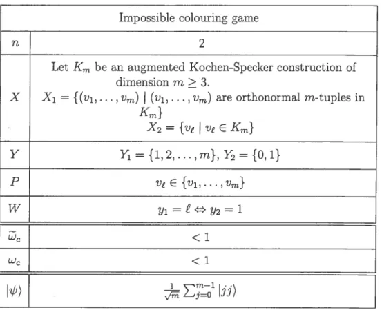
Alice and Bob face in the impossible colouring pseudo-telepathy game is given in table 4.1: Alice receives an orthonormal in-tuple of vectors V1, V2,... , V. Bob receives a single vector v E {v1, V2,.. . , Vm}. Alice outputs Yi E {1, 2,. .. , indicating which of the in vectors of lier input is assigned colour 1. Bob outputs a
bit assigning a colour to his vector. The winlling condition is that Alice and Bob assign the same colour to the vector that they receive in common. It is necessary to use an augmented Kochen-Specker construction of definition 4.1.1 in order to ensure that every vector appears in at Ïeast one instance of the game (although a modification of the game, where we can ask Alice to colour an n-tuplet, where n < in, does not require the use of the augmented Kochen-$pecker construction).
Unlike other pseudo-telepathy games, it is not straightforward to find X1 and X2, because it depends on the augmented Kochen-Specker construction that is used. It would be interesting to calculate these values.
As mentioned earlier, the pseudo-telepathy game based on the Kochen-Specker theorem appeared as early as 1983. Since then, other authors have explored the topic: [Ara99], [MA99] and [RWO4].
Impossible colouring garne
n 2
Let Km be an augmented Kochen-Specker construction of dimension in> 3.
X X1 = {(vi,.. . , Vm) (y1, . . . , U) are orthonormal m-tuples in Km} X2 = {v ve E K} Y Y1 {1, 2,... , m}, Y2 = {O, 1} P W Yi=Y2=’ :; <1 wc <1 1 m—i b) 31)
Table 4.1: Impossible colouring game 4.1.1 A Quantum Winning Strategy
Theorem 4.1.2. Let Gtm be the impossible cotouring game. Then wq(Gm) = 1.
; m—i..
Proof. The player s strategy is to share the state b) =
—
jj). After
receiving their input, Alice and Bob do the following:
1. Alice performs a measurement in the basis Ba = {vi),.. . , Vm)}. $he outputs the index i corresponding to the measured vector.
2. Bob augments the set {v)} to a basis 3b = {ve), wi),.. ., w_’)} of Rtm, and measures in the basis given by Bb. If the outcome is v, he outputs 1, and outputs O otherwise.
To show that this quantum strategy works, we first remark that since the bases
Wb) = Wb,O, Wb,1,... j Wb,m_1) E Bb, m-1 m-1 Z(jVa)(j)Wb) = Va.jWb, (4.1) j=o i=o m-1 = Z37Wb.j (4.2) i=o = (YaWb). (4.3)
The probability that Alice measures v and Bob measures v is given by:
m—1 2 m—1 2 = (jVj)(jV (4.4) (4.5)
fi
i=t = d’ (4.6)10,
i#?We see that the winning condition y; = £ Y2 = 1 is aiways met. This
completes the proof that wq(Gm) = 1.
D
4.1.2 Classical Success Proportion
Theorem 4.1.3. Let Gtm be the impossibte cotonring gaine. Then (Gm) < 1. Proof. Any classical deterministic strategy is a colouring with the properties of definition 4.1.1. Yet the set of vectors used, those of an augmented Kochen-Specker construction of dimension m, may not be coloured in this way; 50 Alice and Bob
cannot have a cassicaÏ winning strategy. D
4.1.3 Special Case of the Impossible Colouring Game
We have presented a infinite family of pseudo-telepathy games based on the Kochen-$pecker theorem. It is interesting to mention the particular case where
m = 3 (table 4.2). For the quantum strategy, Alice and Bob share an entangled
qutrit pair
I)
= (OO) + 11) + 22)). This is interesting as this entangled stateof dimension 9 is the srnallest known state used for a two-party pseudo-telepathy game. In fact, we know for sure that this is the smallest possible state for a two party pseudo-telepathy game [BIVITO4].
Impossible colouring game (m = 3)
n 2
Let K3 he an augmented Kochen-$pecker construction of dimension 3.
X1 = {(v, v, vk) (vi, v,vk) are orthonormal triples in K3}
X2 = {v v E K3} Y Y={1,2,3},Y={O,1} P Vt E {u,v,vk} W c <1
:
Table 4.2: Impossible colouring game (m = 3)
4.2 The Distributed Deutsch-Jozsa Game
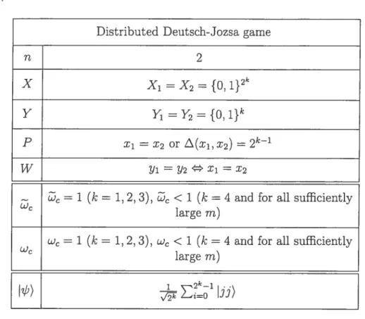
This pseudo-teÏepathy game, based on the Deutsch-Jozsa problem [DJ92], was first presented in [BCT99]. The game uses a parameter k, which determines the size of the game. The task that Alice and Bob face is the following (see table 4.3,
which makes use of definition 4.2.1): they each receive an input bit string of length
2k, with the promise that either their inputs are identical, or they differ in exactly
haif of the positions. They must each output a hit string of length k, such that their outputs are identical if and onÏy if their inputs are identical. Originally, there was only an asymptotic bound known onthe amount of communication required for
classical players to have a winning strategy; thus we could not say for sure which values of k give rise to a pseudo-telepathy game. A few years later, an analysis showed that for k = 4, this game is a pseudo-telepathy game (see section 4.2.2).
Definition 4.2.1. The Hamming Weight of a binary strillgX = x1x2. . . {O, 1}
is denoted A(x) and deflned as:
=
As a consequence, we have that O < (x) <n.
4.2.1 A Quantum Winning Strategy
Theorem 4.2.1. Let Gk be the distribnted Dentsch-Jozsa game. Then wq(Gk) 1. Proof. The player’s strategy is to share the state /‘) =
ii).
Afterreceiving his input x = . . . each player j does the following:
1. apply the unitary transformation S given by S(j)) = (-1)j)
2. apply H to each qubit
3. measure the quhits to obtain yj = yy . . .y’
4. output yj
35
Distributed Deutsch-Jozsa game
n 2
Ï
Xi=X2={O1}2kY Y1=Y2={O,1}k
P x1 x2 or L(x1,r2) = 21e_1
W Y1 = Y2 Xi =
= 1 (k = 1, 2, 3), < 1 (k = 4 and for ail sufflciently
C
large m)
= 1 (k = 1, 2, 3), w, < 1 (k = 4 and for ail siifficiently
C
large m)
Table 4.3: Distributed Deutsch-Jozsa garne Lemma 4.2.2. Let x) be a basis state oJn qubits. Then
= (-1)z)
(47)
where x• z is the bitwise inner product ofx and z, modulo 2, and the sum is over
alt z {O, 1}.
Proof. For a single qubit, we have HO) = I0ii)
and H1) IO)—)i) and so for x) a single qubit,
H
-x)
By hnearity, for x) = Xi . . . x) a basis state,
V’ (1\Z1Z1±...XnZn
z
which can be summarized by
H®x)
= _1)z)
D Now, consider the resulting state afrer step 1 of the quantum strategy:
—1
=
In step 2, both players apply H. By lemma 4.2.2, if
j)
is a basis state of k qubits:2k
H®j)
= (4.8)
where L.
j
is the bitwise inner product of L andj,
modulo 2. So,H®2k) = 1()x3+x3 (1 Z(_1)3u))
(
(_1)3v)) 2k_12k1 t2k_1 = ((_1)+x+iu+iv) nv) 2u=O v=O \j=O
J
The amplitude c of u) y) in H®2k b) determines the probability that y = u and Y2 u. From here, we have two cases:
= x2. Suppose that u u. The amplitude c of u)v) in H02) is: = 1
2k 1
=
L
Where the last une follows by the following argument: we know that
j
u + j.uj
ue
j•v (mod2)andthatj.uej.v=j.(uev). Sinceuu,we have that u u 0. Therefore,
j.
(ue
u) 0 (mod 2) for exactly haif the values ofj
andj
(u C e) 1 (mod 2) for the other haif of the values ofj.
• Hence the winning condition is always satisfled if
• A(xi,x2) = : Suppose that u = u. The amplitude c of u)u) in H®2b) is:
c = 1 22 . 2k_1 = — Z(1)+ 2 =0 Since (x1, x2) = 2k1
implies that x + O (mod 2) for haif valiles of
j
and x + x 1 (mod 2) for the other half ôf the values ofj.
Hence the winning condition is always satisfied if A(x1, x2) 2k—1
L
4.2.2 Classical Success Proportion
The following theorem states that if the parameter k is chosen large enough, this game cannot be won with certainty by classical players. It appeared in a slightly different context in [BCW98].
Theorem 4.2.3. Let Gk be the distributed Deutsch-Jozsa game. Then the amount of commumcation required for ctassical players to win the game is in 2(2’).
But this theorem doesn’t help if we want to know which values of k yield a pseudo-telepathy game. Originally, the authors of
[BCT991
knew that the game had a classical winning strategy for k = 1, 2. They conjectured that this was notthe case for k = 3. However, in [GWO2], the authors prove that there is a cÏassical
winning strategy for k = 3, hence the following theorem:
Theorem 4.2.4. Let Gk be the distTibuted Deutsch-Jozsa game. Then (Gc) = 1
if k E {1,2,3}.
Then, the idea was to show that for k = 4, there was no possibility of a clas
sical winning strategy. By using a.n argument based on graph theory, as well as a computer-assisted case analysis, it was finally shown in [GWTO3] that for k = 4,
there is no classical winning strategy:
Theorem 4.2.5. Let Gk be the distributed Deutsch-Jozsa game. Then (Gk) < 1 if k = 4.
So we know that for k = 4, the distributed Deutsch-Jozsa game is a pseudo
telepathy game. By theorem 4.2.3, we also know that if we choose k larger than a certain threshold k0, then we have a pseudo-telepathy game. However, it is an open question to determine the value of k0. In particular, we don’t even know if k = 5 yields a pseudo-telepathy game!
4.3 The Magic Square Game
The magic square game was presented by Aravind [AraO2, AraO3], who built on work by Mermin [Mer9Od]. The game is also presented in [CHTWO4j.
A magie square is a 3 x 3 binary array that has the property that the sum of each row is even and the sum of each column is odd. Such a square is magic since it cannot exist: suppose we calculate the parity of the nine entries. According to the rows, the parity is even, yet according to the columns, the parity is odd, which is a contradiction.
The task that the players face while playing the garne is the following: Alice is
asked to give the entries of a row and Bob is asked to give the entries of a column.
The winning condition is that the parity of the row must be even, the parity of
agree. Because a classical strategy would have to assign fine entries to a magie square, which is impossible, we know right away that there is no classical winning strategy. The game is described in table 4.4, where y = r1r2r3 (r is used for rows)
and Y2 = c1c2c3 (e is llSed for columns). It is interesting to note that this game is
promise-free according to definition 3.2.5.
Magie square game
n 2
X X1={1,2,3},X2r{1,2,3}
Y Y1=Y2={0,1}3
P none
v3
w i-1 r 0 (mod 2), c 1 (mod 2)
r2 = c1 8 :; 8 wc ‘) (0011) — 0110) — 1001) + 1100))
Table 4.4: Magie square game
4.3.1 A Quantum Winning Strategy
Theorem 4.3.1. Let G be the magie square game. Then wq(G) = 1.
Proof The players share the state b) = (0011)
— 0110) — 1001) + 1100)).
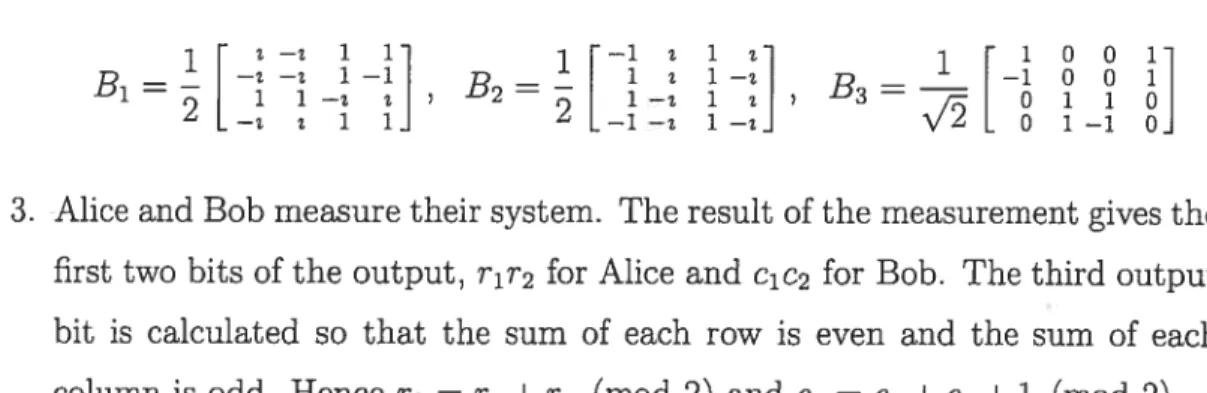
After receiving their inputs (x1 for Alice, x2 for Bob, the players do the following: 1. Alice perforrns the unitary transformation given by the matrix A1 (where ‘i
denotes \/Eï): 7 iOOl 1 2 iii 1_1_1_1 A 0—z 10 A — — i—ii A — 11—11 i7 0210’ -2 2 i—i—i’ 1—111 v2 i c 0 z —i 1 1 —i 1 —1 —1 —1
2. Bob performs the unitary transformation given by the matrix B,:
in—z
11 1—12127 1001D — I — — 1—1 u — 1 z 1—21 — —1 0 0 1
-‘--1—I 1 , 1—il z’ 3_7Z 0110
L—z z 1 1 —1—z 1—z] VZ 0 1—1 0
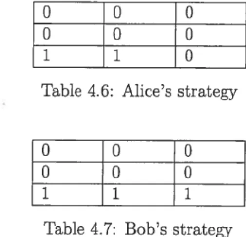
3. Alice and Bob measure their system. The resuit of the measurement gives the first two bits of the output, r1r2 for Alice and c1c2 for Bob. The third output bit is caÏculated 50 that the sum of each row is even and the sum of each
column is odd. Hence r3 = r1 +r2 (mod 2) and e3 = e1 + c2 + 1 (mod 2).
To show that this strategy works, we consider fine cases that correspond to the possible questions x = x1, x2. In each case, we show that the piayer’s final
answer satisfies the winning condition. Because of step 3, we know that the row a.nd column parity conditions are satisfied. After some tedious calculations that we omit here, ve are able to show that indeed r12 = c in ail nine cases. D
The reader might wonder where the unitary transformations A1, A2, A3, B1,32
and 33 corne from. The answer is that they corne from a 3 x 3 array of observables
(table 4.5), each observable defining a measurernent.
Ux®Uy Jy®Gx Uz®Jz
Gy ®Oz Oz ® O•y J1 0 J1
o_z O u1 O u O u2
Table 4.5: A 3 x 3 array of observables Here, u1, u, u denote the PauL matrices:
01 0—z 1 0
u1 = , o_y , o_z =
10 z 0 0—1
The measurement outcome for each observable is O or 1. The operators in each row and in each column commute pairwise, which means that they can be rneasured simultaneously, the resuit being a three-bit string. Since the product along a.ny row is I O I, the outcome for any row is even, and since the product along any column is —I O I, the outcome for any column is odd.