HAL Id: hal-01961218
https://hal.archives-ouvertes.fr/hal-01961218
Submitted on 6 May 2021HAL is a multi-disciplinary open access archive for the deposit and dissemination of sci-entific research documents, whether they are pub-lished or not. The documents may come from teaching and research institutions in France or abroad, or from public or private research centers.
L’archive ouverte pluridisciplinaire HAL, est destinée au dépôt et à la diffusion de documents scientifiques de niveau recherche, publiés ou non, émanant des établissements d’enseignement et de recherche français ou étrangers, des laboratoires publics ou privés.
Optimal due date quoting for a risk-averse
decision-maker under CVaR
Liangyan Tao, Desheng Dash Wu, Sifeng Liu, Alexandre Dolgui
To cite this version:
Liangyan Tao, Desheng Dash Wu, Sifeng Liu, Alexandre Dolgui. Optimal due date quoting for a risk-averse decision-maker under CVaR. International Journal of Production Research, Taylor & Francis, 2018, 56 (5), pp.1934-1959. �10.1080/00207543.2017.1394587�. �hal-01961218�
See discussions, stats, and author profiles for this publication at: https://www.researchgate.net/publication/321496089
Optimal due date quoting for a risk-averse decision-maker under CVaR
Article in International Journal of Production Research · December 2017
DOI: 10.1080/00207543.2017.1394587 CITATIONS 4 READS 153 4 authors, including:
Some of the authors of this publication are also working on these related projects:
Master of Science in English on Supply Chain Management and LogisticsView project
Advances in Production Management Systems (APMS 2021), call for papers and proposals of special sessionsView project Sifeng Liu
Nanjing University of Aeronautics & Astronautics
101PUBLICATIONS 558CITATIONS SEE PROFILE Alexandre Dolgui IMT Atlantique 832PUBLICATIONS 11,605CITATIONS SEE PROFILE
Optimal due date quoting for risk-aversion decision maker under
CVaR
Liangyan Taoa,b, Desheng Dash Wuc, b*, Sifeng Liud,a , Alexandre Dolguie
a.College of Economics and Management, Nanjing University of Aeronautics and Astronautics, Nanjing 210016, China;
b. Stockholm Business School, Stockholm University, Stockholm, SE 106 91, Sweden c. Management School of University of Chinese Academy of Sciences, Beijing 100864, China
d. Centre for Computational Intelligence, De Montfort University, Leicester, LE1 9BH, UK; e. Ecole des Mines de Nantes, IRCCYN, UMR CNRS 6597, La Chantrerie, 4, rue Alfred Kastler - B.P.
20722, F-44307 NANTES Cedex 3, France
Abstract: This paper investigates a due date quoting problem for a project with stochastic duration taking the decision maker’s risk attitude into consideration. The project profit is defined as the difference between the price and the cost that is comprised of production cost, and penalty on earliness and tardiness. Conditional risk at value (CVaR) is employed to describe the decision maker’s risk aversion. In fixed price contract, when the unit production cost is not smaller than the unit penalty on earliness, the optimal due date increases with the increase of the decision maker’s risk aversion and the unit penalty on delay, as well as the decrease of the unit penalty on earliness. Furthermore, when the price is proportional to the due date and the slope is not greater than the unit penalty on tardiness, the optimal due date is smaller than that in fixed price keeping other parameters constant. We then compare the optimal due date in different parameter setting, where the penalty coefficient of earliness is negative or zero respectively. Finally, a case study is conducted to validate the proposed model.
2
1 Introduction
Meeting delivery date(due date) has always been one of the most important objectives in scheduling, supply chain management, and project management in today’s fiercely competitive society(Shabtay et al. 2010). In general, jobs completed after due date always incur tardiness penalties which may consist of compensation of customers, overtime work, delayed delivery costs, etc. For example, the delay of B787 has made Boeing company suffer from extra costs, lost and delayed revenues, loss of customers’ and investors’ confidence, and top management’ reshuffle(Elahi, Sheikhzadeh and Lamba 2014).While jobs that completed prior to the due date may bring about earliness costs including storage costs, spoilage and depreciation and so on. The earliness penalty is prevalent in just in time (JIT) production system. In general, an early due date always stimulates customers to place more orders but may be easy to incur tardiness penalties. In contrast, a late due date may have adverse effect on orders (Guhlich, Fleischmann and Stolletz 2015) but reduce tardiness penalties. Therefore, setting an appropriate due date relates to the success of a project (Park et al. 2010). Specially, trade-off should be took into account when setting due date.
There are two stream of literature on due date settings: due date assignment in machine scheduling and due date quoting in supply chains. A growing body of literature exists in the area of due date assignment in machine scheduling. The main idea is to set due date for every job and then determine an optimal sequence in order to minimize cost(Elimam and Dodin 2013), the weighted number of tardy jobs(Rasti-Barzoki and Hejazi 2013) or to fulfill other objectives( for more details, we refer to Lauff and Werner 2004, Keskinocak and Tayur 2004). With regard to the due date rule, the simplest one is common due date (CON) rule(Panwalkar, Smith and Seidmann 1982) where all jobs are assigned the same due date. Moreover, when job content (e.g. the processing time or the number of operations) affects the due dates, some researchers proposed Slack due date (SLK), total-work-content (TWK), Number of operation (NOP), different due date with no restriction (usually referred to as DIF), etc. Taking special conditions (such as position-dependent deteriorating jobs (Yin et al. 2014), learning effect (Lu et al. 2014), controllable process time (Shabtay, Steiner G and Zhang 2016) into consider, there occur lots of new models in recent years. For example, different from most existing literature assuming independent jobs and constant job duration, Gordon, Strusevich and Dolgui (2012) imposed precedence constraints and controllable processing time on job set. Gordon and Strusevich (2009) addressed a due date assignment (DDA) problem in which the duration of a job hinges on the position in processing sequence. Shabtay D (2016) advanced DDA model by consideringthe restricted due date, namely the due date cannot exceed a predefined value, and proposed a pseudo-polynomial algorithm to solve this problem.
The other strand of literature relating to due date is due date quoting in supply chain or project management. Dumond and Mabert(1988) are the first to address the problem of due date setting for new projects that arrived randomly over time. They compared four due date setting rules, i.e. mean flow due date, number of activities due date rule, critical path time
due date rule and scheduled finish time due date rule with project mean completion time, mean lateness, standard deviation of mean lateness and total tardiness as performance measure, respectively. But in their experiment design, the duration of the project is constant. In addition to some common factors, such as shop status and the size of order, considered during the process of making lead-time promising, Slotnick(2014) incorporated reputation effects that depend on the firm’s delivery performance in lead-time optimization model to balance the attractiveness of short lead time with the possible degradation of reputation resulting from the increased likelihood of tardiness. Guhlich et.al (2015) constructed an integrating model for due date quoting and schedule in an assemble-to-order system under limited assembly capacity and intermediate material. The goal of the integrated model is to answer whether to accept an order and to choose the quoted due date for an accepted order, and to schedule the accepted orders so as to meet the due date. However, all lead time in this paper are constant, neglecting to consider the uncertainty of the lead time, which may arise in practical. Pan and Choi (2013) presented a agent based negotiation and decision making approach to address price and delivery time issue in a three-echelon MTO fashion supply chain. They modeled the negotiation process as optimization model so as to minimize the total cost. The delivery time was determined by cooperation game while the price was attained by competitive negotiation. Pekgün and Griffin (2008) studied the price and due date decision of a firm facing customers who were sensitive to price and due date. They modeled this issue as Stackelberg game and compared the performance of decentralized setting (price being made by market while lead-time by production department) and centralized setting. However, the cost of holding or lateness penalty is neglected in this model. Nguyen and Wright (2015) established a model to address lead-time quoting problem of service enterprises or make to order system with time-varying and lead-time sensitive demand, facilitating the understanding of the interrelationships among lead time, capacity, demand and the total profit. For a comprehensive review concerning order promising (due date assignment) , we refer to Mansouri and Gallear(2012).
Aforementioned literature reviews reveals that the risk attitude of decision makers has received less attentions in due date assignment, because they often suppose a risk-neutral project manager. This is not sufficient for a project with stochastic duration. Besides, most of the previous research assumes that price and due date are interactive, neglecting to consider production cost. In reality, production cost, price, duration and due date always interplay simultaneously. Moreover, taking unproven technology, human performance variability, and natural disruptions into consideration(Zhu, Bard and Yu 2007), the duration of a project is stochastic, instead of the deterministic assumption in previous literature concerning due date quoting. In these regards, the contributions of this paper are concluded in threefold aspect. Firstly, we construct a due date setting model for a project (job) with stochastic duration taking both tardiness and earliness into account. Secondly, the decision maker’s risk attitude is incorporated by means of Conditional value at risk (CVaR). Thirdly, we analyze the influence of construct
4
type (fixed price or variable price in terms of due date), penalty coefficient of earliness (negative, zero or positive) on due date.
The study is motivated by the industrial circumstance in which a risk-averse decision maker should set due date for a project with stochastic duration facing penalty on earliness and tardiness while the price depends on the due date. We formulate this problem as an optimization equation to maximize CVaR that is the performance measure. As an alternative measure of risk, CVaR(Rockafellar and Uryasev 2000) is known to have better properties than Value at Risk (VaR) and thus widely applied in addressing stochastic optimization arising from stochastic scheduling problem(Sarin ,Sherali and Liao 2014), inventory management(Luo ,Wang and Chen 2015), breast cancer therapy(Chan ,Mahmoudzadeh and Purdie 2014), etc. In this paper, we employ CVaR to incorporate decision maker’s risk attitude into the due date setting problem. First we assume the price is independent of the due date, three theorems are given to present the optimal due date and to reveal the effects of different kinds of parameters, such as penalty coefficient, the risk averse degree of decision maker, on due date. After that, we study the scenario where the price is sensitive to the due date. This phenomenon is common in realty, for example faster deliveries can be promised at higher cost (Mansouri and Gallear 2012). Finally, we compare the optimal due date in different parameter setting, where the penalty coefficient of earliness is negative or zero, which means there is reward or no penalty on earliness, respectively.
The rest of the paper is organized as follows. Section 2 presents the due date promising model with CVaR maximized under the circumstance where the price is fixed. Conversely, when the price hinges on the due date, the optimization model is given in Section 3, followed by the analysis of the effect of penalty coefficient of earliness on due date in Section 4. Section 5 is a case study, followed by some conclusions and research prospects in Section 6.
2、The due date optimization model with CVaR maximized under fixed price contract 2.1 Problem description
Due date is one of the most important decisions that the project manager should take into consideration during the planning stage of the development process when a firm should bid a project (Hsiau and Lin 2009). The problem addressed here is that a project manager have to set due date for a project with stochastic duration considering penalty, production cost and price simultaneously. Specially, the penalty consists of penalty on both earliness and tardiness, as just in time has been a prevalent production strategy in recent decades, which requires that jobs should be completed as close to their due dates as possible(Gordon, Strusevich and Dolgui 2012). Otherwise,
the early completion results in storage cost while late completion incurs penalty. Hence the penalty on both earliness and tardiness will be induced in this model. Additionally, the due date decision is also associated with the duration. It is difficult to meet an early due date if the duration is long. To sum up, the due date optimization model need to balance the cost, the penalty, and the duration.
The problem studied here is summarized as: a risk-averse decision maker quotes a due date for a project with stochastic duration. The objective is to maximize performance, measured by
CVaR while taking production cost, penalty and the duration into account. The notation is shown as follows:
Notion
B
The fixed contract price
The random duration of a project, whose cumulative distribution function (CDF) is( )
F
that is differentiable on support (0, ∞)u
The mean completion time of a project, i.e.u
E
( )
, whereE
is the expectation operator.
The constant pertaining to the unit cost of the project 1
The penalty cost coefficient of the early completion 2
The penalty cost coefficient of the late completiond
x
The due date which is the decision variable( , )
x
d
The revenue of the project **
,
f v
d d
x
x
The subscriptf v
,
denote the optimal due date under fixed price and variable price,respectively
2.2 The profit of the project
The cost considered here could be catalogued as production cost and penalty. With respect to production cost, the cost associated with the development of the project is supposed to be determined by the completion time (duration). A small mean completion time always needs more labor, crashing, machines, leading to high cost per time unit. Conversely, a late mean time always makes the unit cost less. The unit cost regarding completion time is defined as
u
, consequently, the production cost is defined as:
d
C
u
. (1) The larger the mean of completion time is, the smaller the production cost coefficient is. This definition is conforming to the law of the diminishing marginal returns, similar to the assumption of Shabtay, Steiner and Zhang (2016), where the resource consumption function is defined as( )
( )
kd b
b
, (2) whered
is the processing time,b
is the assigned resource,
is the workload, andk
are positive parameters. Without loss of generality, we letk
1
.As mentioned above, the JIT manufacturing pattern is prevailing in recent decades, so both the early completion and the late completion will be charged. The penalties for the early completion and the late completion are constructed as
C
e
1(
x
d
) ,
C
l
2(
x
d)
, respectively.When the due date is
x
d, combining the production cost, the penalties and the fixed contract price, we obtain the profit of the project
( , )
x
d
, which is a function ofx
d and the random completion time
: 1 2 2 2 1 2(
, )
(
)
(
)
(
)(
)
d d d d dx
B
x
x
B
x
x
(3)6
where
z
max z
{ , 0}
. 2.3 Performance measure: CVaRFrom (3), we know
( , )
x
d
is also a random variable, CVaR is thus employed to measure the performance. According to the work of Rockafellar and Uryasev2000, the CVaR for the decision problem pertaining to the due date is1
{
[
( (
d, )
, 0)]}
v R
CVaR
max v
E min
x
v
, (4)where
(0,1]
represents the risk aversion degree of risk for the project managers. The smaller
is, the more risk averse the decision maker is (see Chen, Xu and Zhang 2009).The decision problem is to optimize the due date to obtain maximum CVaR. The optimal due date is P1
arg
0{
(
, )}
d d x v dx
max
max g x v
, Where 2 2 1 2 0 1 2 0 1 1 2 2 01
(
, )
[
(
)(
) ]
( )
1
1
[
(
)]
( )
[
(
)]
( )
1
1
[
(
) )]
( )
[
(
) ]
( )
d d d d d d d x d x d x d x dg x v
v
v
B
x
x
dF
u
v
v
B
x
dF
v
B
x
dF
u
u
v
v
B
x
dF
v
B
x
dF
u
u
The solution of P1 differs in different scenarios where the relationship between
u
and
1 is different. The first condition is the case where the unit cost is the same as the unit penalty onearly completion, i.e 1
u
. The optimal due date and CVaR is given in Theorem 1.Theorem 1 When 1
u
, the optimal due date under fixed price contract and CVaR are* 1 1 * * 1 1 2
(1
),
f f d dx
F
v
B
x
, respectively.The proof is given in Appendix. From Theorem 1, we can find that
(1) The due date is increasing with the increasing of risk aversion degree, i.e. the decreasing of
. In other words, a risk aversion manager prefers a late due date. For example, if
approach 0, i.e the decision maker is most risk averse, the optimal due date is close toF
1(1)
whereF
1( )
is the inverse cumulative distribution function of the project’s duration.(2) A bigger penalty cost coefficient on delay (
2) brings a later due date since it is better to avoid delay due to high penalty. Setting a later due date is a good choice to reduce delay.(3) Additionally, the bigger the penalty coefficient of early completion (
1) is, the smaller the due date is. This is because that an early completion will suffer high penalty and a tight due date makes it hard to complete a project before the due date. (4) With respect to the optimal CVaR, CVaR decreases as the risk aversion degree ofdecision maker increases. On the contrary, a big penalty cost coefficient on early completion
1results in bad CVaR performance.If the unit production cost is bigger than penalty cost coefficient of early completion, the following result holds, shown in Theorem2 with proof in Appendix.
Theorem 2 When 1
u
, the optimal due date and CVaR under fix contract price are* 1 1 * * 1 1 1 1 2
(1
),
(
)
( )
f f d dx
F
v
B
x
F
u
, respectively. If let 1u
, we find that the optimal due date and CVaR is the same as the one in Theorem 1. The optimal CVaR is smaller comparing to the one of Theorem1. Moreover CVaR increases asu
decrease. This is easy to understand because low production cost always lead to high revenue.
When 1
u
, we derive new results shown in Theorem 3, which are more complicate.Theorem 3 When 1
u
, the optimal due date and CVaR under fixed contract price are1 1 1 2 2 1 * 1 2 1 2 1 2
(
)
(1
) (
)
(
)
,
f dF
F
u
u
x
* * 2 1 1 2 1 1 1 2 1 2 1 2(
)
1
1
(
)
(
)
(
)
(1
)
2
2
2
f dx
v
B
F
F
u
u
, respectively. When we set 1u
, we find that the optimal due date and CVaR in Theorem 3 are the same as the one in Theorem 1.Compared to the results in theorem 1 and 2, we find that the due date in this case is smaller due to high penalty on early completion(
1). Consequently, setting a early due date lower the possibility of finishing ahead of schedule, thus leading to low penalty on early completion. In sum, the optimal due date is sensitive to unit production costu
, unit penalty cost
1
,
2
, the risk aversion
and the cdf of completion timeF
1( )
.8
In reality, the price is always sensitive to the due date. Generally, a project manager will charge high price for a project with a short due date, since manufactures may have to recruit more employers, conduct more investment and pay more overtime salary aiming to shorten the due date. Since many customers are reluctant to buy a product with long due date, a long due date often weaken the manufactures’ competition, leading to the broken up with the customer in the competitive market. Thus, a trade-off between price and due date should be taken into account in the due date optimization problem. This section incorporates the customers’ due date-price trade-off to extend the model in Section 2, which is more realistic and applicable. First, we present the trade off curve proposed by Moodie(1999), shown in Figure1. The customers’ maximum accepted price for the early due date (denoted as EDD) is PEDD, while the maximum accepted price for the late due date (denoted as LDD) is PLDD. The segment between EDD and LDD shows that the price decreases with the increase of due date.
Insert Figure 1 about here
From Figure1, we deduce the formula of the trade-off curve as following:
1 2
0
*
,
0,
d d d dB
x
EDD
B
B
k x
EDD
x
LDD
x
LDD
wherek
PEDD PLDD
LDD EDD
,B
2
B
1
k EDD
*
,B
1
PEDD
.When
x
d
EDD
, the situation is the same as the one in section 2 with fixed price contract. Whenx
d
FDD
, the firm prefer to not produce anything, since the due date exceeds the customers’ maximum accepted due date and the price is 0.3.1 The optimal due date under linearly variable contract price
First we only consider the circumstance where
B
B
2
k x
*
d, 0
x
d, neglecting to consider the constraintEDD
x
d
LDD
,which will be analyzed in the following. In this situation, the relation between price and due date is linear, thus we call this linearly variable contract price. The optimal due date and CVaR are conforming to the following three theorems, whose proofs are listed in the Appendix.Theorem 4 When 1
u
, the optimal due date and CVaR under due date-sensitive price( is also referred to variable price contract) are(1) If
2
k
, * 1 1 1 2(
)
[1
]
dk
x
F
, * 1 1 2 1 1 2(
)
(
)
[1
k
]
v
B
k
F
, respectively. (2) If
2
k
,x
*d
0
,v
*
B
2
(
1
2)
F
1(1
)
, respectively.From Theorem 4, when we find that the optimal due date is decreasing in the increasing of
k
. In other words, the more the price is sensitive to the due date, the earlier the due date is quoted when
2
k
. Moreover, the minimal due date isF
1[1
]
when
2=k
.Theorem 5 When 1
u
, the optimal due date and CVaR under variable price contract are(1) If
2
k
, * 1 1 1 2(
)
[1
]
d vk
x
F
, * * 1 2(
1)
d(
1)
(1
)
vv
B
k x
F
u
, respectively. (2) If
2
k
,x
*d
0
,v
*B
2(
2)
F
1(1
)
u
, respectively. If let 1u
in theorem 5, we find that the optimal due date and CVaR in theorem 5 are the same as those in theorem 4, which means that theorem 4 is a special case of theorem 5. Compared to the results in fixed price contract in Section 2, the optima due date in variable price contract is smaller when
2
k
(i.e.* 1 * 1 1 1 1 2 1 2
(
)
[1
]
[1
]
d d vk
fx
F
x
F
). This is becausethe customer pays more for short due date, encouraging the firm to quote a short due date, in the circumstance where unit delay cost (
2) is bigger than the price increased by unit shorten due-date, namely the slope of the trade-off curve (k
).When
2
k
, which means unit delay cost is smaller than the price’s increment incurred by the unit decrement of due date, the optimal due date is 0. In this situation, the firm would like to set a minimum due date, since the penalty for delay will be complemented by the increment of price. This phenomenon implies the customer have to increase the unit penalty cost for delay.If the penalty on early completion is bigger than the unit production cost, the results are given in theorem 6.
Theorem 6 When 1
u
, the optimal due date and CVaR under variable price contract are(1) If
2
k
, * 1 1 1 2 2 1 1 2 1 2 1 2)
(
)
(1
) (
)
(
)
d vk
k
F
F
u
u
x
, * 2 1 1 2 1 1 1 2 1 2 1 2(
)
1
1
(
)
(
)
(
)
(1
)
2
2
2
dx
k
k
v
B
F
F
u
u
, respectively.10
(2) If
2
k
there is no meaning due to the meaningless of 1 21 2
)
(
k
)
F
.Compared to the results in Theorem 3, we find that the optimal due date in variable price
contract is smaller than the one in fixed price when
2
k
,because1 1 1 1 1 2 1 2 1 2 1 2 1 2 1 2
)
)
(1
)
(1
k
),
(
(
k
F
F
F
F
. Furthermore, if let=0
k
, the results in theorem 6 is the same as theorem 3.3.2 The optimal due date under piecewise variable price contract
Next, taking the constraint
EDD
x
d
LDD
into account, the relation between price and due date is piecewise, we then need to explore this problem in the following three scenarios. (1) Scenario 1: 1u
In this scenario where the unit production cost is equal to the unit penalty on early completion, the optimal due date is sensitive to different parameters comprising
F
1(1
)
,1 1 1 2
(
)
[1
k
]
F
,
2, k
.etc. Specially, the results vary in three different cases, which areclassified by the relation among
F
1(1
)
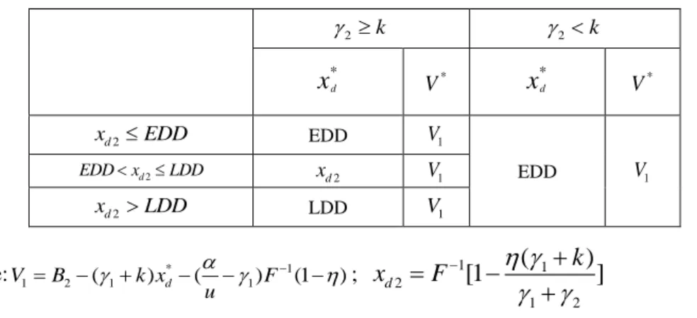
, EDD and LDD. The concrete analysis on the three different cases is given in the Appendix.Combined the results of three different cases in the Appendix, the optimal due date and CVaR
corresponding to Scenario 1( 1
u
)is given in the Table 1. Insert Table 1 about hereWhen 2 k, we always have a smaller due date compared to the optimal due date when
2 k
if the other parameters remain constant. The reason is that the added price incurred by unit decreased due date is bigger than the penalty on the unit delay. In this case, the firm is inclined to quote a early due date so as to obtain high contract price, while the CVaR decreases as the due date increases.
The decision on due date is more complex when 2 k , which is depending on many
scenarios which are comprised by different relation among F1(1),EDD and other parameters.
Generally, the larger the value of 1
(1 )
F is , the bigger the due date is quoted. Because a
bigger value of 1
(1 )
to select a bigger due date to avoid high delay penalty. Regarding the revenue, the optimal CVaR decreases as the value of 1
(1 )
F sees an increase.
(2) Scenario 2: 1
u
The optimal due date is depending on different parameters, including
F
1(1
)
,1 1 1 2
(
)
[1
k
]
F
,
2, k
.etc. Specially, the results vary in three different cases, which areclassified by the relation among
F
1(1
)
, EDD and LDD. The concrete analysis on the three different cases is given in the Appendix.Based on the results of three different cases in the Appendix, the optimal due date and CVaR in scenario2 is shown in Table 2.
Insert Table 2 about here
We try to draw some conclusion from table 8. In generally, if we let
be equal to, we find
that the results of Scenario 2 is the same as the one in Scenario 1. Compared to the case when
2 k
, the quoted due date is smaller in the case when 2 k and the other parameters are the
same. As for revenue, the CVaR when 1
u
is smaller than the one when 1u
when all other parameters remain the same, since the increase of unit production cost (
) resultes in high production cost.(3)Scenario 3: 1
u
When the unit production cost is smaller than the unit penalty on early completion, the
optimal due date is depending on different parameters, including
2 1 1 2 (1 ) F , 1 1 1 2 2 1 1 2 1 2 1 2 ( )F (1 ) ( )F ( ) u u
(denoted as
x
d3),
2, k
.etc. Specially, the results vary inthree different cases, which are classified by the relation among
2 1 1 2 (1 ) F , EDD and LDD. Case 1 2 1 1 2
(1
)
F
EDD
12
When
0
x
d
EDD
,B
B
1.From the proof of theorem 3 in Appendix, we know the optimal due date is:(1) If
x
d3
EDD
,then the optimal due date and the CVaR are* * * * 1 2 1 1 1 1 1 2 1 , | ( ) ( ) 1 d d d B x v B x v x EDD V v F F u u , respectively.
(2) If
x
d3
EDD
, then the optimal due date and the CVaR are* * 1 1 3 2 2 2 1 2
,
(
)
(1
)
d d dx
x
v
B
x
F
u
, respectively.When
EDD
x
d
LDD
,B
B
2
kx
d.From the proof of theorem 6 in Appendix, we know the optimal due date is shown in Table 3.Insert Table 3 about here
When
x
d
LDD
,B
0
.The firm decides to produce nothing. The optimal due date depends on the relationship between the value of CVaR associated with the due datex
d fallingin the interval (0, EDD) and the value of CVaR when
EDD
x
d
LDD
. Specially, the firm will quote the due date with largest CVaR. For example, ifv
2
v
3, the due date will be set as3 d
x
. Case 2 2 1 1 2(1
)
EDD
F
LDD
In this situation, the optimal due date and CVaR are given in Table 4, according to the proof 3and 6 in Appendix.
Insert Table 4 about here
The optimal due date is set at the point whose CVaR is bigger. For example, if v6 v7, the optimal due date is EDD. Otherwise, the firm has to quote LDD as the due date.
Case 3 2 1 1 2
(1
)
F
LDD
In this situation, the optimal due date and CVaR are given in Table 5, according to the proof 3and 6 in Appendix.
Insert Table 5 about here Since 1 1 2 2 2 1 2 2 1 2 1 2 2 ( ) ( ) (1 ) [ ( ) ( ) (1 )] ( ) [ ( ) ] ( )( ) 0 B k LDD F B kEDD k EDD F u u
B kEDD k LDD B kEDD k EDD
k LDD EDD ,
the optimal due date is LDD in this case where
F
1(1
)
is bigger than LDD. If the project manager quotes a due date, which is bigger than LDD, the firm will not get order. On the other hand, if the firm selects a tight due date, which is smaller than LDD, it will suffer a high delay cost. Although a small due date will bring high contract price, the penalty on delay is bigger than the increase in price due to 2 k. Moreover, the firm is vulnerable to delay, becauseF
1(1
)
is so big that it is difficult to finish the project before a small due date. LDD is thus an optimal due date.4.The influence of penalty coefficient for early completion 1 4.1 Fixed contract price
If there is no penalty on the early completion ( 1 0), the firm’s decision on due date absolutely is different from the case presented above. According to the theorem 2, the firm will quote
F
1(1)
that is the maximum duration as the due date. Because the contract price is independent on the due date, meanwhile the firm will not be charged for early completion, the firm prefers to set the due date as late as better to decrease the possibility of overdue, leading to zero penalty cost on delay. Obviously, this case is scarce in practical. Furthermore, we consider an extreme scenario where 1 0, namely the customer encourages the firm to delivery earlier. The optimal due date is given as follows: When 1 20,according to the proof of theorem 2, the optimal due date is
F
1(1)
, that means the firm will complete the project beforeF
1(1)
, while the CVaR is1 1 1 1 (1) ( 1) (1 ) B F F ;
When 1 20,according to the proof of theorem 2, the optimal due date is
1 1 1 2
(1
)
F
, while the CVaR is 1 1 1 1 1 11 2 (1 ) ( ) (1 ) B F F . 2 1
implies that the penalty on delay is bigger than the award on early completion, thus the firm tends to set the due date as late as possible, whereas 2 1, the firm is apt to select a early due date and obtain a bigger CVaR.
14
When the contract price is dependent on the due date, specially, the function is suggested as
1
2 * d, 0 d (1)
BB k x x F . We identify the optimal due date in various scenarios according to
the proof of theorem 5 since the conditions of the theorem 4 and theorem 6 do not exist when
1 0 .
When 10,2kaccording to the proof of theorem 5, the optimal due date is 1 2 (1 k) F
, which is bigger than 1 1 1 2 ( ) (1 k ) F
due to the non-existing penalty
on early completion. Meanwhile 1 2
(1
k
)
F
is smaller than
F
1(1)
, because asmall due date can get a bigger contract price. The CVaR is
1 1 2 1 2 ( ) (1 k) (1 ) B k F F ;
When 10,2kaccording to the proof of theorem 5, the optimal due date is 0,
while the CVaR is 1
2 ( 2) (1 )
B F
u
. In this case, the smaller the degree of risk aversion is, the bigger the CVaR is . This is due to the small penalty on delay compared to the award on early due date( 2 k).
When 1 0, according to the proof of theorem 5, the optimal due date is given in the following table.
Insert Table 6 about here
From Table 6, we can conclude some interesting insights. For example, when1 k 0,
indicating that the award on early completion is bigger than the award on small due date, the firm mostly tend to quote big due date so as to purse the award on early completion, excepting the situation where 1 20.Furthermore,
1 1 1 2 ( ) (1 k ) F
in Table 6 is bigger than the one in theorem 5
as 1 1 ' 1 1 1 1 1 ' 2 2 1 2 ( ) ( ) (1 k ) (1 k) (1 k ) (1 ) F F F F ,where 1 '
represents a negative1. Quoting a
bigger due date aims to gain the reward on early completion.
4.3 Piecewise variable price contract
The case studied above neglect to consider the customer’s accepted due date, including EDD and LDD. If the function between contract price and due date is given as Figure 1, we have to study the optimal due date in the scenario where there are a negative1or 1with zero value. The specific results are given in Table 7,8,9 respectively.
Insert Table 7 about here Insert Table 8 about here Insert Table 9 about here
5. Case study
Taizhou Jindeli Furniture Co.Ltd, located in Zhejiang Province, China, has specialized in design and production of European and American classical furniture since 1995. There are
widespread exclusive shops of this company in most Chinese large and medium-sized cities, such as Beijing, Shanghai. The production system is the mixture of Make to Order and Make to Stock. For some products with fluctuate demand and high inventory costs, make to order is a good choice. This paper takes a type of sofa (coded as 908-50) as an example to demonstrate the application of this proposed model. Product 908-50 is a typical “make to order” product because it is difficult to forecast the demand and the holding cost is high. The history data reveals that the duration of Product 908-50 is normal distribution. The mean and standard deviation is 36 days and 4, respectively, i.e.
~
N
(36, 4)
.5.1 CVaR in fixed price
We consider a situation under which one exclusive shop decides the price with the customer in the first stage. After that, the manufacture deselects the due date. We assume the price is 45,000 CNY( We disguised the amount in this paper for confidentiality),namely
B
45, 000
. The otherparameters are set as
/
u
800,
1
750,
2
1000,
0.95
.Since
/ u
1, according to theorem 2, we derive the optimal due date and CVaR is* 1 1 1 1 2
750*0.95
(1
)
(1
)
36.5,
15, 660
750 1000
f dx
F
F
CVaR
. 36.5 days is thereforethe optimal due date in this case.
To validate the result, we also employ Crystal Ball software to simulate the duration. First, we simulate 100,000 times to get 100,000 random profits. Then according to the following formula, we can calculate the CVaR in different conditions where the due date is different based on the simulated data.
0
arg
{
(
, )},
d d x v dx
max
max g x v
where 11
(
, )
[
]
*
q d i ig x v
v
v
q
,q
100, 000
is the simulation times and
i is the profit of the ith simulation. The relation between CVaR and due date is shown in Figure 2 which shows that 36.5 days is the optimal due date while the optima CVaR is 14824. The error of optimal CVaR between simulation method and the theorem 2 is 5.7 %, i.e.15660 14768
5.7%
15660
.
Insert Figure 2 about here 5.2 CVaR under linearly variable price
Contrary to the situation in section 5.1, the price is not always fixed. In this section, taking the effect of the due date on the price into consideration, we assume the price is
45, 000 200*
d, 0
dB
x
x
. According to theorem 4, we obtain the optimal due date andCVaR: * 1 1 1 1 2
(
)
0.95(750 200)
[1
]
[1
]
36.0,
10875
750 800
dk
x
F
F
CVaR
.16
As mentioned above, the optimal due date decreases as the slope k increases, which is shown in Figure 3.
Insert Figure 3 about here 5.3 CVaR under stepwise variable price
In this section, we study the optimal due date decision problem when the price is given as the following formula. The other parameters are the same as the one above.
45, 000
0
35
45, 000 200*
,
40
0,
d d d dx
EDD
B
x
EDD
x
LDD
x
LDD
Because 1 1 (1 ) (1 0.95) 32.7 35F F EDD , according to scenario 2, we derive the
optimal due date and CVaR is * 1 1
1 2 min{ , [1 ]} min{35,36.5} 35 d x EDD F , * 1 1 1 d ( 1) (1 ) 14114 CVaR B x F .
Furthermore, if the customer encourages early finish, namely
1
0
, referring to the results in Section 4, we can obtain the optimal due date:1 * 1 1 35, 0 200 40, 200 1000 (1 0.95) 32.7, 1000 d x F 6. Conclusion
This paper aims to establish an optimization model concerning due date quoting for a project with stochastic duration taking decision maker’s risk aversion into consideration. In detail, the paper defines a project’s profit as the interval between contract price and the costs comprising production cost, penalty on earliness and tardiness. Since the duration is stochastic, the profit associated with the due date and the duration is also random. CVaR is thus employed to describe the decision maker’s risk attitude and regarded as the objective of the due date determining model. More specifically, we explore the due date decision problem in two scenarios: the first one is fixed price contract where the price is independent on the due date and the other is variable price contract(including linear function and piecewise function) which is sensitive to due date. Generally, one can charge more for an early due date.
In the first case where price is fixed, we derive the optimal due date in three different cases.
When 1
u
, i.e. the unit production cost is no smaller than the unit penalty on earliness, theoptimal due date is * 1 1
1 2
(1
)
f dx
F
, implying that (1) when the decision maker is mostdelay, i.e.
2is large, always leads to a later due date; (3) The optimal due date decreases as the unit penalty on earliness early completion increases. When 1u
, the optimal due date is1 1 1 2 2 1 * 1 2 1 2 1 2 ( ) (1 ) ( ) ( ) f d F F u u x
. In the second case the relation between due date and
price is piecewise, shown in Figure 1. The optimal due date is depending on different parameters
including
F
1(1
)
, 1 1 1 2(
)
[1
k
]
F
,
2, k
.etc. At last, we analyze the influence of penaltycoefficient of earliness (negative, zero) on due date.
There are some rooms for improving. In this paper, we do not consider the resource constraint. However, the resource is limited in reality, therefore we should incorporate resources constraint in the model. Besides, we only formulate the due date decision problem in state environment ignoring the interaction between the new project and the existing project. If the project(order) arrives over time, we need to answer whether to accept the new order, what is the optimal due date and how to schedule the orders accordingly.
Acknowledgments
This work is supported by the Ministry of Science and Technology of China under Grant 2016YFC0503606, by National Natural Science Foundation of China (NSFC) grant [grant Nos. 71471055; 71671090;71671091and 91546102], by Key Research Program of Frontier Sciences, CAS under Grant No. QYZDB-SSW-SYS021, and a Marie Curie International Incoming Fellowship within the 7th European Community Framework Programme under Grant No. FP7-PIIF-GA-2013-629051. At the same time, the authors would like to acknowledge the partial support of Chinese Scholarship Council, Jiangsu Innovation Program for Graduate Education under Grant number KYZZ15_0092 and the Fundamental Research Funds for the Central Universities under grant number NP2015208.
References
Shabtay D, Itskovich Y, Yedidsion L, et al. 2010. “Optimal due date assignment and resource allocation in a group technology scheduling environment”. Computers & Operations Research 37(12): 2218-2228.
18
Analyzing Boeing's Outsourcing Program for Dreamliner (B787)”. Knowledge and Process
Management 21(1): 13-28.
Guhlich H, Fleischmann M, Stolletz R. 2015. “Revenue management approach to due date quoting and scheduling in an assemble-to-order production system”. OR Spectrum 37(4): 951-982.
Park M, Lee D, Shin K, et al. 2010. “Business integration model with due-date re-negotiations”. Industrial Management & data systems 110(3): 415-432.
Elimam A A, Dodin B. 2013. “Project scheduling in optimizing integrated supply chain operations”. European Journal of Operational Research 224(3): 530-541.
Rasti-Barzoki M, Hejazi S R. 2013. “Minimizing the weighted number of tardy jobs with due date assignment and capacity-constrained deliveries for multiple customers in supply chains”.
European Journal of Operational Research 228(2): 345-357.
Lauff V, Werner F. 2004. “Scheduling with common due date, earliness and tardiness penalties for multimachine problems: A survey”. Mathematical and Computer Modelling 40(5): 637-655.
Keskinocak P, Tayur S. 2004. “Due date management policies”. Handbook of quantitative
Supply Chain Analysis. Springer US: 485-554.
Panwalkar S S, Smith M L, Seidmann A. 1982. “Common due date assignment to minimize total penalty for the one machine scheduling problem”. Operations research 30(2): 391-399.
Yin Y, Wu W H, Cheng T C E, et al.2014. “Due-date assignment and single-machine scheduling with generalised position-dependent deteriorating jobs and deteriorating
multi-maintenance activities”. International Journal of Production Research 52(8): 2311-2326. Lu Y Y, Li G, Wu Y B, et al. 2014. “Optimal due-date assignment problem with learning effect and resource-dependent processing times”. Optimization Letters 8(1): 113-127.
Shabtay D, Steiner G, Zhang R. 2016. “Optimal coordination of resource allocation, due date assignment and scheduling decisions”. Omega, http://dx.doi.org/10.1016/j.omega.2015.12.006.
Gordon V, Strusevich V, Dolgui A. 2012. “Scheduling with due date assignment under special conditions on job processing”. Journal of Scheduling 15(4): 447-456.
Gordon V S, Strusevich V A. 2009. “Single machine scheduling and due date assignment with positionally dependent processing times”. European Journal of Operational Research 198(1): 57-62.
Shabtay D. 2016. “Optimal restricted due date assignment in scheduling”. European Journal
of Operational Research 252(1): 79-89.
Dumond J, Mabert V A. 1988. “Evaluating project scheduling and due date assignment procedures: an experimental analysis”. Management Science 34(1): 101-118.
Slotnick S A. 2014. “Lead-time quotation when customers are sensitive to reputation”.
International Journal of Production Research 52(3): 713-726.
Guhlich H, Fleischmann M, Stolletz R. 2015. “Revenue management approach to due date quoting and scheduling in an assemble-to-order production system”. OR Spectrum 37(4): 951-982.
Pan A, Choi T M. 2013. “An agent-based negotiation model on price and delivery date in a fashion supply chain”. Annals of Operations Research 1-29.DOI 10.1007/s10479-013-1327-2
Pekgün P, Griffin P M, Keskinocak P. 2008. “Coordination of marketing and production for price and lead time decisions”. IIE transactions 40(1): 12-30.
Nguyen T H, Wright M. 2015. “Capacity and lead-time management when demand for service is seasonal and lead-time sensitive”. European Journal of Operational Research 247(2): 588-595.
Mansouri S A, Gallear D, Askariazad M H. 2012. “Decision support for build-to-order supply chain management through multiobjective optimization”. International Journal of Production
Economics 135(1): 24-36.
Zhu G, Bard J F, Yu G. 2007. “A two-stage stochastic programming approach for project planning with uncertain activity durations”. Journal of Scheduling 10(3): 167-180.
Rockafellar R T, Uryasev S. 2000. “Optimization of conditional value-at-risk”. Journal of
risk 2: 21-42.
Sarin S C, Sherali H D, Liao L. 2014. “Minimizing conditional-value-at-risk for stochastic scheduling problems”. Journal of Scheduling 17(1): 5-15.
Luo Z, Wang J, Chen W. 2015. “A risk-averse newsvendor model with limited capacity and outsourcing under the CVaR criterion”. Journal of Systems Science and Systems Engineering, 24(1): 49-67.
Chan T C Y, Mahmoudzadeh H, Purdie T G. 2014. “A robust-CVaR optimization approach with application to breast cancer therapy”. European Journal of Operational Research 238(3): 876-885.
Hsiau H J, Lin C W R. 2009. “A fuzzy pert approach to evaluate plant construction project scheduling risk under uncertain resources capacity”. Journal of Industrial Engineering and
Management 2(1): 31-47.
Moodie D R. 1999. “Due date demand management: negotiating the trade-off between price and delivery”. International Journal of Production Research 37(5): 997-1021.
Chen Y, Xu M, Zhang Z G. 2009. “a risk-averse newsvendor model under the CVaR criterion”. Operations Research 57(4): 1040-1044.
20 Appendixes P1
arg
0{
(
, )}
d d x v dx
max
max g x v
, Where 1 2 2 01
1
(
, )
d[
)]
( )
[
(
) ]
( )
d x d d x dg x v
v
v
B
x
dF
v
B
x
dF
u
1.The proof of Theorem 1 Proof: In this situation, 1
u
, so 1 2 2 01
1
(
, )
d[
)]
( )
[
(
) ]
( )
d x d d x dg x v
v
v
B
x
dF
v
B
x
dF
u
Case 1.
v
B
1 dx
. In this case,1 2 2 0 1 1 ( , ) d( ) ( ) [ ( ) ] ( ) d x d d x d g x v v v B x dF v B x dF u
Thusg x v
(
d, )
1
1
0
v
Case 2.
v
B
1 dx
. We can derive that2 2 2 2 1 ( d, ) B xd v[ d ( ) ] ( ) u g x v v v B x dF u
Then 2 2 2 2(
, )
1
(
, )
1
[1
(
)],
0
d d dg x v
B
x
v
g x v
F
and
v
v
u
. Letg x v
(
d, ')
0
v
hold, we have ' 1 2 1 2(
d)
d(
)
(1
)
v x
B
x
F
. Furthermore,(
d, )
g x v
is increasing with the increase ofv
whenv
v
'
, whileg x v
(
d, )
decreases in theinterval between
v
' andB
1 dx
.Let
v x
(
d)
*be the optimal CVaR of P1 for fixedx
d. Combining Case 1and Case 2, weobserve that
![Table A.1 the optimal due date and CVaR when EDD x d LDD in Scenario 1 2 k 2 k * x d V * x *d V * 1 1 1 2( )[1k ]F EDD EDD B 2 ( 1 k x) *d EDD B 2 ( 1 k x) *d11 1 2( )[1k ]EDDF LDD 1 11 2( )[1k ]F B](https://thumb-eu.123doks.com/thumbv2/123doknet/12247229.319761/39.892.144.752.151.364/table-optimal-date-cvar-edd-ldd-scenario-eddf.webp)