A general symmetry-preserving observer for aided attitude heading reference systems

(1)

HAL Id: hal-00495853

https://hal-mines-paristech.archives-ouvertes.fr/hal-00495853

Submitted on 29 Jun 2010

HAL is a multi-disciplinary open access

archive for the deposit and dissemination of

sci-entific research documents, whether they are

pub-lished or not. The documents may come from

teaching and research institutions in France or

abroad, or from public or private research centers.

L’archive ouverte pluridisciplinaire HAL, est

destinée au dépôt et à la diffusion de documents

scientifiques de niveau recherche, publiés ou non,

émanant des établissements d’enseignement et de

recherche français ou étrangers, des laboratoires

publics ou privés.

A general symmetry-preserving observer for aided

attitude heading reference systems

Philippe Martin, Erwan Salaün

To cite this version:

Philippe Martin, Erwan Salaün. A general symmetry-preserving observer for aided attitude

head-ing reference systems. 47th IEEE Conference on Decision and Control, Dec 2008, Cancun, Mexico.

pp.2294 - 2301, �10.1109/CDC.2008.4739372�. �hal-00495853�

(2)

A General Symmetry-Preserving Observer for Aided Attitude Heading

Reference Systems

Philippe Martin and Erwan Sala¨un

Abstract— We generalize several recent works on nonlinear observers for aided attitude heading reference systems: we pro-pose a symmetry-preserving nonlinear observer which merges the most common measurements available on an aircraft (alti-tude, Earth-fixed and body-fixed velocity, inertial and magnetic sensors). It can be seen as an alternative to the Extended Kalman Filter, but easier to tune and computationally much more economic. Moreover it has by design a nice geomet-rical structure appealing from an engineering viewpoint. We illustrate its good performance on simulation and experimental results.

I. INTRODUCTION

Aircraft, especially Unmanned Aerial Vehicles (UAV), commonly need to know their orientation and velocity to be operated, whether manually or with computer assistance. When cost or weight is an issue, using very accurate inertial sensors for “true” (i.e. based on the Schuler effect due to a non-flat rotating Earth) inertial navigation is excluded. Instead, low-cost systems –sometimes called aided Attitude Heading Reference Systems (AHRS)– rely on light and cheap “strapdown” gyroscopes, accelerometers and magne-tometers “aided” by position and velocity sensors (for in-stance the velocity vector is given in body-fixed coordinates by an air-data or Doppler radar system, the position/velocity vectors in Earth-fixed coordinates by a GPS engine, the altitude by a barometric altimeter). The various measure-ments are then “merged” according to the motion equations of the aircraft assuming a flat non-rotating Earth, usually with a linear complementary filter or an Extended Kalman Filter (EKF). For more details about avionics, various inertial navigation systems and sensor fusion, see for instance the books [4], [10], [7], [5], [6] and the references therein.

While the EKF is a general method capable of good performance when properly tuned, it suffers several draw-backs: it is not easy to choose the numerous parameters; it is computationally expensive, which is a problem in low-cost embedded systems; it is usually difficult to prove the convergence, even at first-order, and the designer has to rely on extensive simulations. Moreover on the aided attitude heading problem, suitable modifications must be made to make it work with quaternions [11], [9].

An alternative route is to use an ad hoc nonlinear observer as proposed in [19], [13], [8], [14], [12], [1], [16], [17], [15]. In the absence of a general method the main difficulty is of course to find such an observer. In this paper we

The authors are with the Centre Automatique et Syst`emes,

´

Ecole des Mines de Paris, 60 boulevard Saint-Michel, 75272

Paris Cedex 06, FRANCE philippe.martin@ensmp.fr,

erwan.salaun@ensmp.fr

use the rich geometric structure of the flying rigid body problem to derive an observer by the method developed in [3], building up on the preliminary work [2]. We propose a general observer structure able to handle the various possible sensors, and which supersedes the previous works [13], [8], [14], [12], [16], [17], [15]. It has by design a nice geometrical structure appealing from an engineering viewpoint; it is easy to tune, computationally very economic, and with guaranteed (at least local) convergence around every trajectory for low velocity flight. Moreover it behaves sensibly in the presence of magnetic disturbances. We illustrate its good performance on simulation and on preliminary experimental comparisons with the commercial Microbotics MIDG II system.

II. PHYSICAL EQUATIONS AND MEASUREMENTS

A. Motion equations

The motion of a flying rigid body (assuming the Earth is flat and defines an inertial frame) is described by

˙ q=1 2q∗ ω ˙ v= v × ω + q−1∗ A ∗ q + a ˙h = $q ∗ v ∗ q−1_{, e} 3% where

• q is the quaternion representing the orientation of the

body-fixed frame with respect to the Earth-fixed frame

• ω is the instantaneous angular velocity vector

• vis the velocity vector of the center of mass with respect

to the Body-fixed frame

• A = ge3 is the (constant) gravity vector in

North-East-Down coordinates (the unit vectors e1, e2, e3point

respectively North, East, Down)

• a is the specific acceleration vector, i.e. all the

non-gravitational forces divided by the body mass.

• h is the altitude of the center of mass

More generally we could use ˙x= q ∗ v ∗ q−1, where x is

the position of the center of mass in the Earth-fixed frame, instead of the last equation.

The first equation describes the kinematics of the body, the second is Newton’s force law. It is customary to use quaternions (also called Euler 4-parameters) instead of Euler angles since they provide a global parametrization of the body orientation, and are well-suited for calculations and computer simulations. For more details about this section, see any good textbook on aircraft modeling, for instance [18], and section VIII in [14] for useful formulas used in this paper.

CCCaaannncccuuunnn,,, MMMeeexxxiiicccooo,,, DDDeeeccc... 999---111111,,, 222000000888

(3)

B. Measurements

We have four triaxial sensors plus the pressure sen-sor, providing thirteen scalar measurements: 3 gyros

mea-sure ωm= ω + ωb, where ωb is a constant vector bias;

3 accelerometers measure a; 3 magnetometers measure

yb= q−1∗ B ∗ q, where B = B1e1+ B3e3 is the Earth

mag-netic field in NED coordinates; the velocity vector yv= v

in the body-fixed frame is provided by some air-data or

Doppler radar system; the velocity vector yV= V is provided

by the navigation solution of a GPS engine; a barometric

sensor provides the altitude measurement yh= h. All these

measurements are of course also corrupted by noise. It is possible to include more parameters to model the sensors imperfections, see [16], [17], [15]. For simplicity we have considered here only gyros biases.

C. The considered system

To design our observers we therefore consider the system

˙ q=1 2q∗ (ωm− ωb) (1) ˙ v= v × (ωm− ωb) + q−1∗ A ∗ q + a (2) ˙h = $q ∗ v ∗ q−1_{, e} 3% (3) ˙ ωb= 0 (4)

whereωm and a are seen as known inputs, together with the

output     yv yV yB yh    =     v q∗ v ∗ q−1 q−1∗ B ∗ q h    . (5)

III. CONSTRUCTION OF THE OBSERVER

A. Invariance of the system equations

There is no general method for designing a nonlinear observer for a given system. When the system has a rich geometric structure, namely invariance with respect to sym-metry group, the ideas in [3] provide a constructive method to this problem and simplify the analysis of the error system. Several translational and rotational groups have been considered for the aided attitude estimation problem [13], [8], [14], [12], [16], [17], [15]. Nevertheless as soon as we also consider position/velocity measurements in both the Earth-fixed and body-fixed frames translations acting on the velocities must be ruled out, see the discussion in IV. We therefore consider the following transformation group generated by constant rotations and translation in the

body-fixed and Earth-body-fixed frames

ϕ_(p 0,q0,h0,ω0)     q v h ωb    =     p0∗ q ∗ q0 q−1₀ ∗ v ∗ q0 h+ h0 q−1₀ ∗ ωb∗ q0+ ω0    =     ˜ q ˜ v ˜h ˜ ωb     ψ_(p 0,q0,h0,ω0)     ωm a A B    =     q−1₀ ∗ ωm∗ q0+ ω0 q−1₀ ∗ a ∗ q0 p0∗ A ∗ p−10 p0∗ B ∗ p−10    =     ˜ ωm ˜ a ˜ A ˜ B     ρ_(p₀_,q₀_,h₀_,ω₀₎     yv yV yB yh    =     q−1₀ ∗ yv∗ q0 p0∗ yV∗ p−10 q−1₀ ∗ yB∗ q0 yh+ h0    =     ˜ yv ˜ yV ˜ yB ˜ yh    .

There are 3+ 3 + 1 + 3 = 10 parameters: the two unit

quaternions p0 and q0, the scalar h0 and the R3-vector ω0.

The group law& is given by

    p1 q1 h1 ω1    &     p0 q0 h0 ω0    =     p0∗ p1 q0∗ q1 h0+ h1 q−1₁ ∗ ω0∗ q1+ ω1    .

The system (1)–(4) is of course invariant by the transforma-tion group since

˙˜q = p0∗ ˙q ∗ q0= p0∗ ( 1 2q∗ ω) ∗ q0 =1 2(p0∗ q ∗ q0) ∗ (q −1 0 ∗ ω ∗ q0) = 1 2q˜∗ ˜ω ˙˜v = q−1 0 ∗ ˙v ∗ q0 = (q−1₀ ∗ v ∗ q0) × (q−1₀ ∗ ω ∗ q0) + q−1₀ ∗ a ∗ q0 + (p0∗ q ∗ q0)−1∗ (p0∗ A ∗ p−10 ) ∗ (p0∗ q ∗ q0) = ˜v × ˜ω+ ˜q−1∗ ˜A∗ ˜q + ˜a ˙˜h = ˙h = $q ∗ v ∗ q−1_{, e} 3% = $ ˜q ∗ ˜v ∗ ˜q−1, ˜e3% ˙˜ ωb= q−10 ∗ ˙ωb∗ q0= 0,

whereas the output (5) is compatible since     ˜ v ˜ q∗ ˜v ∗ ˜q−1 ˜ q−1∗ ˜B∗ ˜q ˜h    = ρ(p0,q0,h0,ω0)     v q∗ v ∗ q−1 q−1∗ B ∗ q h    .

B. Construction of the general invariant pre-observer

We solve for(p0, q0, h0, ω0) the normalization equations

p0∗ q ∗ q0= 1

p0∗ ei∗ p−10 = ˜ei with i= 1, 2, 3 (6)

h+ h0= 0

q−1₀ ∗ ωb∗ q0+ ω0= 0

where ( ˜e1, ˜e2, ˜e3) defines a new orthonormal frame. The

moving frameγ(q, h, ωb, e1, e2, e3) is then defined by

q0= q−1∗ p−10

h0= −h

ω0= −p0∗ q ∗ ωb∗ q−1∗ p−10

!777ttthhh IIIEEEEEEEEE CCCDDDCCC,,, CCCaaannncccuuunnn,,, MMMeeexxxiiicccooo,,, DDDeeeccc... 999---111111,,, 222000000888 WWWeeeAAA111333...222

(4)

where p0 represents the rotation between the two frames

(e1, e2, e3) and ( ˜e1, ˜e2, ˜e3). We slightly generalize the

con-struction in [3] since we normalize not only with respect to ϕ but also with respect to ψ.

We can then find the 10 scalar invariant errors which correspond to the projections of the output error

ρ_{γ( ˆq,ˆh, ˆ}_ω b,e1,e2,e3)   ˆ yv ˆ yV ˆ yB  − ρ_{γ( ˆq,ˆh, ˆ}_ω b,e1,e2,e3)   yv yV yB  

on the new frame ( ˜e1, ˜e2, ˜e3) and to the output error for yh

which is directly invariant. We get

Evi= $ ˆq ∗ ( ˆyv− yv) ∗ ˆq−1, ei%

EVi= $ ˆyV− yV, ei%

EBi= $B − ˆq ∗ yB∗ ˆq−1, ei%

Eh= ˆh − h,

where i= 1, 2, 3. We detail how to get Evi:

$ρ_{γ( ˆq,ˆh, ˆ}_ω b,e1,e2,e3) ' ˆ yv ( − ρ_{γ( ˆq,ˆh, ˆ}_ω b,e1,e2,e3) ' yv ( , ˜ei% = $p0∗ ˆq ∗ ˆyv∗ ˆq−1∗ p−10 − p0∗ ˆq ∗ yv∗ ˆq−1∗ p−10 , ˜ei% = $ ˆq ∗ ˆyv∗ ˆq−1− ˆq ∗ yv∗ ˆq−1, p−10 ∗ ˜ei∗ p0% = $ ˆq ∗ ( ˆyv− yv) ∗ ˆq−1, ei%.

We get also the 9 scalar complete invariants which corre-spond to the projections of

φ_{γ( ˆq, ˆv, ˆ}_ω_b_,e₁_,e₂_,e₃₎'vˆ( and ψ_{γ( ˆq, ˆv, ˆ}_ω_b_,e₁_,e₂_,e₃₎

)

ωm

a *

on the new frame( ˜e1, ˜e2, ˜e3). We find

Iviˆ = $ ˆq ∗ ˆv ∗ ˆq−1, ei%

I_ω_mi= $ ˆq ∗ (ωm− ˆωb) ∗ ˆq−1, ei%

Iai= $ ˆq ∗ a ∗ ˆq−1, ei% where i= 1, 2, 3.

Notice that Iviˆ, Iωmi, Iai, Evi, EVi, EBi’s and Ehare functions

of the estimates and the measurements. Hence they are known quantities which can be used in the construction of the preobserver. It is straightforward to check they are indeed invariant. For instance,

$ ˆq ∗ ˆv ∗ ˆq−1, ei%

= $p0∗ ˆq ∗ ˆv ∗ ˆq−1∗ p−10 , p0∗ ei∗ p−10 %

= $(p0∗ ˆq ∗ q0) ∗ (q−1₀ ∗ ˆv ∗ q0) ∗ (p0∗ ˆq ∗ q0)−1, ˜ei%.

To find invariant vector fields, we solve for w(q, v, h, ωb)

the 10 vector equations    Dϕγ(q,v,ωb,e1,e2,e3)     q v h ωb        · w(q, v, h, ωb) =     ˜ ei 0 0 0    ,     0 ˜ ei 0 0    ,     0 0 e7 0    ,     0 0 0 ˜ ei     i= 1, 2, 3. Since    Dϕ(p0,q0,h0,ω0)     q v h ωb        ·     δ q δ v δ h δ ωb    =     p0∗ δ q ∗ q0 q−1₀ ∗ δ v ∗ q0 δ h q−1₀ ∗ δ ωb∗ q0    ,

this yields the 10 independent invariant vector fields

(i= 1, 2, 3)     ei∗ q 0 0 0    ,     0 q−1∗ ei∗ q 0 0    ,     0 0 e7 0    ,     0 0 0 q−1∗ ei∗ q    .

Indeed for instance the equations p0∗ δ q ∗ q0= ˜ei gave us

δ q= p−1₀ ∗ ˜ei∗ q−10 = (p−10 ∗ ˜ei∗ p0) ∗ (q0∗ p0)−1= ei∗ q.

It is easy to check that these vector fields are invariant. The general invariant preobserver then reads

˙ˆq =1 2qˆ∗ (ωm− ˆωb) + 3

∑

i=1 ' 3

∑

j=1 (lvi jEv j+ lVi jEV j+ lBi jEB j) + lhiEh ( ei∗ ˆq ˙ˆv = ˆv × (ωm− ˆωb) + ˆq−1∗ A ∗ ˆq + a + ˆq−1∗ 1 3

∑

i=1 ' mhiEh + 3

∑

j=1 (mvi jEv j+ mVi jEV j+ mBi jEB j) ( ei 2 ∗ ˆq ˙ˆh = $ ˆq∗ ˆv∗ ˆq−1_{, e} 3% + 3

∑

j=1 (nv jEv j+ nV jEV j+ nB jEB j) + nhEh ˙ˆ ωb= ˆq−1∗ '3

∑

i=1 ' 3

∑

j=1 (ovi jEv j+ oVi jEV j+ oBi jEB j) + ohiEh ( ei(∗ ˆq, where the lvi j, lVi j, lBi j, lhi, mvi j, mVi j, mBi j, mhi, nv j, nV j,

nB j, ovi j, oVi j, oBi j, ohi’s and nh are arbitrary scalars which

possibly depend on Evi, EVi, EBi, Eh, Iviˆ, Iωmi and Iai’s.

Noticing 3

∑

i=1 ' 3

∑

j=1 (lvi jEv j) ( ei= LvEv

where Ev= ˆq ∗ ( ˆv− v) ∗ ˆq−1and Lvis the 3× 3 matrix whose

coefficients are the lvi j’s, and defining EV, EB, LV, LB, Lh,

Mv, MV, MB, Mh, Nv, NV, NB, Nh, Ov, OV, OB and Oh in

the same way, the correction terms can be rewritten with the

matrices E, L, M, N and O such as E = (EvEV EB Eh)T and

LvEv+ LVEV+ LBEB+ LhEh= LE,

and the same notation for M, N and O. Then we can rewrite the preobserver as

˙ˆq =1 2qˆ∗ (ωm− ωb) + (LE) ∗ ˆq (7) ˙ˆv = ˆv × (ωm− ωb) + ˆq−1∗ A ∗ ˆq + a + ˆq−1∗ (ME) ∗ ˆq (8) ˙ˆh = $ ˆq∗ ˆv∗ ˆq−1_{, e} 3% + (NE) (9) ˙ˆ ωb= ˆq−1∗ (OE) ∗ ˆq. (10) 222222999666

(5)

The preobserver is indeed invariant by considering the

pro-jection of the output errors Ev, EV and EB on the frame

(e1, e2, e3). As a by-product of its geometric structure, the

preobserver automatically has a desirable feature: the norm

of ˆq_{is left unchanged by (7), since LE is a vector of R}3_(see

section VIII in [14]). C. Error equations

The state error is given by     η ν λ β    = ϕγ(q,v,ωb,e1,e2,e3)     ˆ q ˆ v ˆh ˆ ωb    − ϕγ(q,v,ωb,e1,e2,e3)     q v h ωb     =     ˆ q∗ q−1− 1 q∗ ( ˆv − v) ∗ q−1 ˆh − h q∗ ( ˆωb− ωb) ∗ q−1    .

It is in fact more natural –though completely equivalent–

to take η= ˆq ∗ q−1 _{(rather than} _η_{= ˆq ∗ q}−1_{− 1), so that}

η(x, x) = 1, the unit element of the group of quaternions.

As we did above it can be easily checked that λ and the

projections of η, ν and β on the frame (e1, e2, e3) are

invariant. Hence for(i, j) = 1, 2, 3,

˙ 3 45 6 $η ∗ ei∗ η−1, ej% = $ ˙η∗ ei∗ η−1− η ∗ ei∗ η−1∗ ˙η∗ η−1, ej% = 2$(−1 2η∗ β ∗ η −1_{) × (η ∗ e} i∗ η−1), ej% + 2$(LE) × (η ∗ ei∗ η−1), ej% $ ˙ν, ei% = $(η−1∗ Ivˆ∗ η) × β + η−1∗ A ∗ η − A, ei% + $η−1∗ (ME) ∗ η, ei% ˙λ = ˙ˆh − ˙h = $Ivˆ− η−1∗ Ivˆ∗ η − η−1∗ ν ∗ η, e3% + (NE) $ ˙β, ei% = $(η−1∗ Iωm∗ η) × β + η −1_{∗ (OE) ∗ η, e} i%.

Since we can write

Ev= η ∗ ν ∗ η−1 EV= Ivˆ− η−1∗ Ivˆ∗ η + ν

EB= B − η ∗ B ∗ η−1 Eh= λ ,

we find as expected that the error system ˙ 3 45 6 η∗ ei∗ η−1= 2(− 1 2η∗ β ∗ η −1_{) × (η ∗ e} i∗ η−1) + 2(LE) × (η ∗ ei∗ η−1) (11) ˙ ν= (η−1∗ Ivˆ∗ η) × β + η−1∗ A ∗ η − A + η−1∗ (ME) ∗ η (12) ˙λ = $Ivˆ− η−1∗ Ivˆ∗ η − η−1∗ ν ∗ η, e3% + (NE) (13) ˙ β = (η−1∗ Iωm∗ η) × β + η −1_{∗ (OE) ∗ η} (14)

depends only on the invariant state error(η, ν, λ , β ) and the

“free” known invariants Ivˆand Iωm, but not on the trajectory

of the observed system (1)–(4). The error system (11)– (14) is invariant by considering the projection of the

equa-tions (11),(12) and (14) on the frame(e1, e2, e3).

The linearized error system around

(η, ν, λ , β ) = (1, 0, 0, 0), i.e. the estimated state equals the actual state, is given by

δ ˙η= −1 2δ β+ (Lδ E) (15) δ ˙ν= Ivˆ× δ β + 2A × δ η + (Mδ E) (16) δ ˙λ = $−Ivˆ× δ η − δ ν, e3% + (Nδ E) (17) δ ˙β = Iωm× β + (Oδ E), (18) where δ Ev= δ ν δ EV= δ ν − 2Ivˆ× δ ν δ EB= 2B × δ η δ Eh= δ λ .

We notice that the normalization equation (6) let us

to consider the velocity error ν in the Earth-fixed frame.

Instead, choosing q−1₀ ∗ ei∗ q0= ˜ei would lead us a velocity

error ˜ν= ˆv − v in the body-fixed frame which seems more

“natural” since the equation (2) is written in body-fixed

coordinates. But in this case, the output error δ EB would

becomeδ ˜EB= 2( ˆq−1∗ B ∗ ˆq) × δ ν; so the error system, and

its convergence behavior, would depend on the trajectory ˆ

q(t).

IV. POSITION WITH RESPECT TO PREVIOUS WORKS

The invariant observer (7)–(10) supersedes several previ-ous works, which are detailed in this section.

A. No velocity measurements: [8]-[14]-[16]

In [8]-[14]-[16] only inertial and magnetic sensors are

used. So the linear acceleration ˙v− v × ω is supposed small

enough to approximate the accelerometers measurements by

ya= −q−1∗ A ∗ q. We recover the observer described in

[8]-[14]-[16] considering only (1) and (4) as the physical system

and ya and yb as the output.

B. Ideal measurements: [1]

The nonlinear complementary filter presented in [1] use ideal measurements: pose estimation (computationally de-manding) and no biases.

C. Transformation incompatible with body-fixed velocity: [17]

In [17] only the Earth-fixed measurements are used. The constructed observer can not be adapted to the body-fixed measurements since with the chosen transformation group

the output yv is not compatible.

D. No body-fixed velocity: [15]

The observer proposed in [15] is written in the Earth-fixed frame because no body-Earth-fixed velocity measurements are considered. We recover this observer transposing (8) in the Earth-fixed frame.

(6)

E. Transformation incompatible with Earth-fixed velocity: [3]

In [3] only the body-fixed measurements are used and no biases are considered. The constructed observer can not be

adapted to the body-fixed measurements since the output yv

is not compatible with the chosen transformation group. F. Particular case: [2]

The observer (7)–(10) generalizes the observer presented in [2]. Indeed we recover it taking

LvEv= −l1Ev− l2Ev× A − l3$Ev, A%A

MvEv= −l4Ev− l5Ev× A − l6$Ev, A%A

and considering no bias and no Earth-fixed measurements.

V. CHOICE OF THE OBSERVER PARAMETERS

Up to now, we have only investigated the structure of the

observer. We now must choose the gain matrices Lv, LV, LB,

Lh, Mv, MV, MB, Mh, Nv, NV, NB, Nh, Ov, OV, OB, Ohto meet

the following requirements locally around any trajectory:

• at a low velocity “normal” flight, which is common for

UAVs in an urban area, i.e. Ivˆ and Iωm are first order

terms: the error must converge to zero and its behavior should be easily tunable; the magnetic measurements should not affect the attitude, velocity and altitude estimations, but only the heading

• at a level flight, i.e. Ivˆ= V1e1+V2e2+ δV3e3 where

V1,V2are constant and Iωm, δV3are first order terms, the

behavior of the roll angle error towards the direction of

Ivˆ, which is the most important estimation for a flight

control, should not be affected by V1,V2,δV3 and any

magnetic disturbance. Therefore we choose LvEv= lvA× Ev LVEV= lVA× EV LBEB= lB$B × EB, A%A MvEv= −mvEv MVEV= −mVEV NhEh= −nhEh OvEv= −ovA× Ev OVEV= −oVA× EV OBEB= −oB$B × EB, A%A

with(lv, lV, lB, mv, mV, nh, ov, oV, oB) > 0 and the other

matri-ces equal to 0. At a low velocity “normal” flight the error system (15)–(18) splits into three decoupled subsystems and two cascaded subsystems:

• the longitudinal subsystem

  δ ˙η2 δ ˙ν1 δ ˙β2  =   0 g∗ (lv+ lV) −1₂ −2g −(mv+ mV) 0 0 −(ov+ oV) 0     δ η2 δ ν1 δ β2  

• the lateral subsystem

  δ ˙η1 δ ˙ν2 δ ˙β1  =   0 −g ∗ (lv+ lV) −1₂ 2g −(mv+ mV) 0 0 ov+ oV 0     δ η1 δ ν2 δ β1  

• the vertical subsystem

δ ˙ν3= −(mv+ mV)δ ν3

• the heading subsystem

)δ ˙η3 δ ˙β3 * = ) −2gB2 1lB −1₂ 2gB2₁oB 0 * ) δ η3 δ β3 * + ) 2gB1B3lB −2gB1B3oB * δ η1

• the altitude subsystem

δ ˙λ = −nhδ λ− δ ν3.

Thanks to this decoupled structure, the tuning of the gains

lv, lV, lB, mv, mV, nh, ov, oV, oB is straightforward. Obviously

the lateral, longitudinal, vertical and altitude subsystems do not depend on the magnetic measurements, so will not be affected if the magnetic field is perturbed. We do not detail in this article how the choice of matrices meet the preceding requirements during a level flight. We only illustrate it through simulation and experimental results.

VI. SIMULATION RESULTS

We first illustrate on simulation the behavior of the invari-ant observer ˙ˆq = 1 2qˆ∗ (ωm− ˆωb) + (LE) ∗ ˆq + α(1 − ' ˆq' 2_{) ˆq} ˙ˆv = ˆv × (ωm− ˆωb) + ˆq−1∗ A ∗ ˆq + a + ˆq−1∗ (ME) ∗ ˆq ˙ˆh = $ ˆq∗ ˆv∗ ˆq−1_{, e} 3% + (NE) ˙ˆ ωb= ˆq−1∗ (OE) ∗ ˆq

with the choice of gain matrices described in section V. The

added termα(1 − ' ˆq'2) ˆq is a well-known numerical trick to

keep' ˆq' = 1. Notice this term is invariant.

We choose here time constants around 20s by

tak-ing lv= lV= 1e − 2, lB= 5.2e − 3, mv= mV = 2.4, nh= 1,

ov= oV= 5.3e − 3, oB= 2.8e − 3 and α = 1. The system

follows the trajectory defined by

a=   .4g ∗ sin(t) .4g ∗ sin(.5t + π/4) −g − .4g cos(.5t)   ω=   .5 sin(.5t) .9 sin(.3t) −.5 sin(.25t)   ωb=   .01 .008 −.01  ,

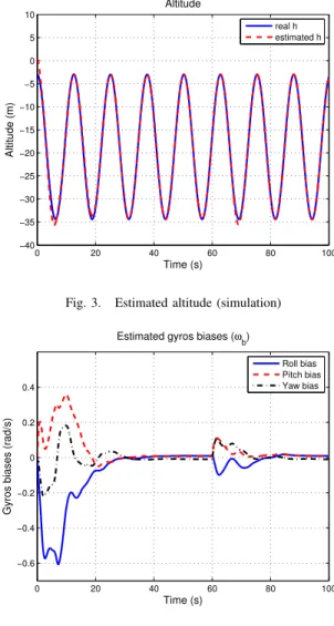
which is representative of a small UAV flight. We see on the Fig. 1–4 the results of the following experiment:

• for t< 40s the observer converges well. Though we

have no proof of convergence but local, the domain of attraction seems to be large enough since the states are initialized far from their true values and the system moves quite fast

• at t= 40s the “GPS correction terms” are switched off,

i.e. the gains lV, mV and oV are set to 0. The observer

still behaves well

• at t = 60s the magnetic field is changed from

B= (1 0 1)T _{to B}_{= (0.5 − 0.8 0.7)}T_{. As expected,}

(7)

0 20 40 60 80 100 −100 0 100 Euler angles Roll angle (°) 0 20 40 60 80 100 −100 0 100 Pitch angle (°) 0 20 40 60 80 100 −100 0 100 Time (s) Yaw angle (°) real φ estimated φ real θ estimated θ real ψ estimated ψ

Fig. 1. Estimated Euler angles (simulation)

0 20 40 60 80 100 −20 0 20 Velocity vx (m/s) 0 20 40 60 80 100 −20 0 20 vy (m/s) 0 20 40 60 80 100 −20 0 20 Time (s) vz (m/s) real v x estimated v x real v y estimated v y real v_z estimated v_z

Fig. 2. Estimated velocity (simulation)

only the estimated yaw angle ψ is strongly affected by

the magnetic disturbance. Because of the coupling terms

Ivˆand Iωm, there is some dynamic influence on the other

variables.

VII. EXPERIMENTAL RESULTS

We do not have yet measurements from an air-data sys-tem, so we will use only Earth-fixed velocity, inertial and magnetic measurements provided by the commercial INS-GPS device MIDG II from Microbotics Inc and altitude measurement given by the barometer module Intersema MS5534B. For each experiment we first save the raw mea-surements from the MIDG II gyros, acceleros and magnetic sensors (at a 50Hz refresh rate), the velocity provided by the navigation solutions of its GPS engine (at a 5 Hz refresh rate) and the raw measurements from a barometer module (at a 12.5 Hz refresh rate). A microcontroller on a development kit communicate with these devices and send the measurements to a computer via the serial port (see Fig. 5). On Matlab Simulink we feed offline the observer with these data and then compare the estimations of the observer to the estimations given by the MIDG II (computed

0 20 40 60 80 100 −40 −35 −30 −25 −20 −15 −10 −5 0 5 10 Altitude Time (s) Altitude (m) real h estimated h

Fig. 3. Estimated altitude (simulation)

0 20 40 60 80 100 −0.6 −0.4 −0.2 0 0.2 0.4

Estimated gyros biases (ω

b)

Time (s)

Gyros biases (rad/s)

Roll bias Pitch bias Yaw bias

Fig. 4. Estimated biases (simulation)

according to the user manual by some Kalman filter). In order to have similar behaviors and considering the units of the raw measurements provided by the MIDG II, we have

cho-sen lV= 2.8e − 5, lB= 1.4e − 6, mV= 9e − 3, nh= 5e − 2,

oV= 4e − 7, oB= 2e − 8 and α = 1 and we initialized the

altitude measurement to 0 at the beginning of the experiment. A. Dynamic behavior (Fig. 6–8)

We wait a few minutes until the biases reach constant values, then move the system in all directions. The observer and the MIDG II give very similar results (Fig. 6–8). To do comparison in the same frame we compare the Earth velocity

provided by the MIDG II and ˆV= ˆq ∗ ˆv ∗ ˆq−1 _{given by our}

observer. We can notice that the estimation of Vz given by

our observer seems to be closer to the real value than the estimation provided by the MIDG II: we know that we let

the system motionless at t= 42s, which is coherent with our

estimated ˆVz.

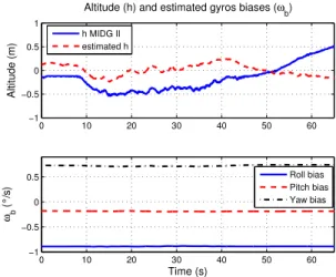
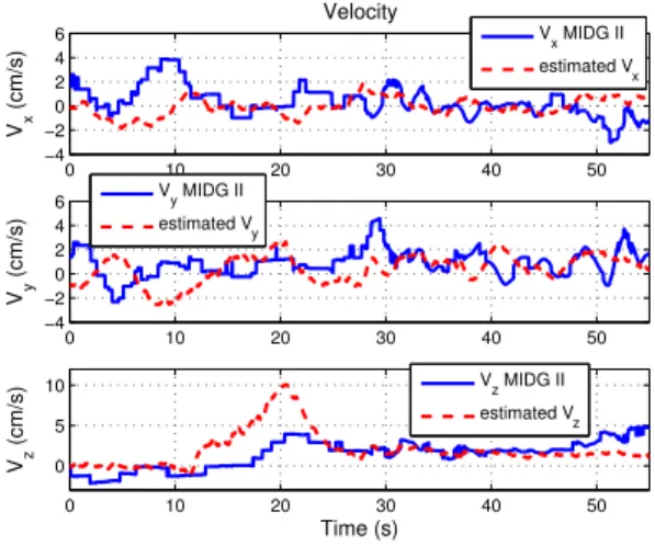
B. Influence of magnetic disturbances (Fig. 9–12)

Once the biases have reached constant values, the system

is left motionless for 60s. At t= 72s a magnet is put close to

(8)

Fig. 5. Experimental protocol 0 10 20 30 40 50 60 −20 0 20 40 Euler angles Roll angle (°) 0 10 20 30 40 50 60 −20 0 20 Pitch angle (°) 0 10 20 30 40 50 60 −150 −100 −50 Time (s) Yaw angle (°) φ MIDG II estimated φ θ MIDG II estimated θ ψ MIDG II estimated ψ

Fig. 6. Estimated Euler angles (experiment)

0 10 20 30 40 50 60 −0.5 0 0.5 Velocity Vx (m/s) 0 10 20 30 40 50 60 −0.5 0 0.5 Vy (m/s) 0 10 20 30 40 50 60 −0.2 0 0.2 Time (s) Vz (m/s) V x MIDG II estimated V_x V_y MIDG II estimated V_y V_z MIDG II estimated V_z

Fig. 7. Estimated velocity (experiment)

0 10 20 30 40 50 60 −1 −0.5 0 0.5 1

Altitude (h) and estimated gyros biases (ω_b)

Altitude (m) 0 10 20 30 40 50 60 −1 −0.5 0 0.5 ωb (°/s) Time (s) h MIDG II estimated h Roll bias Pitch bias Yaw bias

Fig. 8. Estimated altitude and biases (experiment)

0 10 20 30 40 50 0 0.2 0.4 Euler angles Roll angle (°) 0 10 20 30 40 50 0.2 0.4 Pitch angle (°) 0 10 20 30 40 50 −60 −40 −20 0 20 Time (s) Yaw angle (°) φ MIDG II estimated φ θ MIDG II estimated θ ψ MIDG II estimated ψ

Fig. 9. Influence of magnetic disturbances (experiment)

the sensors for 10s. As expected the estimated roll and pitch angles, longitudinal and lateral velocities are not affected by the magnetic disturbance (Fig. 9–10); the MIDG II exhibits a similar behavior. However we notice that the yaw angle estimated by our algorithm is much more affected by the disturbance that the estimation provided by the MIDG II. And thus the estimated vertical velocity and altitude are also perturbed (Fig. 9–11). Indeed for the experiments related to the Fig. 9–11 we used the gain values detailed above, which are constant whatever the norm of the magnetic field is. If the norm of the magnetic measurements change, which means that there is some magnetic disturbance, we would like this to affect the gain values of the magnetic correction terms.

For instance if the norm of yBincreases we want to decrease

the gains lB and oB of the “magnetic correction terms”. A

first possibility is to consider the gains lBand oBdivided by

'yB'1.5, supposing'yB' (= 0. On the Fig. 12 we see that the

estimated vertical velocity, altitude and yaw angle are really less disturbed, and are now close to the estimations given by the MIDG II.

(9)

0 10 20 30 40 50 −4 −2 0 2 4 6 Velocity Vx (cm/s) 0 10 20 30 40 50 −4 −2 0 2 4 6 Vy (cm/s) 0 10 20 30 40 50 0 5 10 Time (s) Vz (cm/s) V_x MIDG II estimated V_x V y MIDG II estimated V y V_z MIDG II estimated V_z

0 10 20 30 40 50

−2 −1 0 1

Altitude (h) and estimated gyros biases (ω

b) Altitude (m) 0 10 20 30 40 50 0 0.2 0.4 0.6 ωb (°/s) Time (s) h MIDG II estimated h Roll bias Pitch bias Yaw bias

0 10 20 30 40 50 −10 0 10 20 Yaw angle ψ ψ (°) 0 10 20 30 40 50 −20 2 4 6 Velocity v_z Vz (cm/s) 0 10 20 30 40 50 −2 −1 0 1 Altitude h Time (s) h (m) ψ MIDG II estimated ψ V_z MIDG II estimated V_z h MIDG II estimated h

Fig. 12. Influence of magnetic disturbances with adapted gains

(experi-ment)

VIII. CONCLUSION AND FUTURE WORKS

In this paper we proposed a general nonlinear observer for aided attitude heading reference systems. It can merge several kinds of measurements from Earth-fixed and body-fixed low-cost sensors. We illustrated its well-behavior and nice properties on simulation and preliminary experimental results. Further work is in progress to implement the observer on a cheap microcontroller, see [16], [15], to demonstrate the computational simplicity of the observer.

REFERENCES

[1] G. Baldwin, R. Mahony, J. Trumpf, T. Hamel, and T. Cheviron. Complementary filter design on the special euclidean group SE(3). In Proc. of the 2007 European Control Conference, 2007.

[2] S. Bonnabel, Ph. Martin, and P. Rouchon. A non-linear symmetry-preserving observer for velocity-aided inertial navigation. In Proc. of the 2006 American Control Conference, pages 2910–2914, 2006.

[3] S. Bonnabel, Ph. Martin, and P. Rouchon. Symmetry-preserving

observers. arxiv.math.OC/0612193, 2007. Accepted for publication in IEEE Trans. Automat. Control.

[4] R.P.G. Collinson. Introduction to avionics systems. Kluwer Academic Publishers, second edition, 2003.

[5] J.A. Farrell and M. Barth. The global positioning system and inertial navigation. McGraw-Hill, 1998.

[6] M.S. Grewal and A.P. Andrews. Kalman filtering : Theory and

Practice using MATLAB. Wiley, second edition, 2001.

[7] M.S. Grewal, L.R. Weill, and A.P. Andrews. Global positioning

systems, inertial navigation, and integration. Wiley, second edition, 2007.

[8] T. Hamel and R. Mahony. Attitude estimation on SO(3) based on direct inertial measurements. In Proc. of the 2006 IEEE International Conference on Robotics and Automation, pages 2170–2175, 2006. [9] Y.M. Huang, F.R. Chang, and L.S. Wang. The attitude determination

algorithm using integrated GPS/INS data. In Proc. of the 16th IFAC World Congress, 2005.

[10] M. Kayton and W.R. Fried, editors. Avionics navigation systems.

Wiley, second edition, 1997.

[11] E.J. Lefferts, F.L. Markley, and M.D. Shuster. Kalman filtering for spacecraft attitude. Journal of Guidance and Control, 5(5):417–429, 1982.

[12] R. Mahony, T. Hamel, and J-M. Pfimlin. Non-linear complementary filters on the special orthogonal group. IEEE Trans. Automat. Control, 2008. To appear.

[13] R. Mahony, T. Hamel, and J.-M. Pflimlin. Complementary filter design on the special orthogonal group SO(3). In Proc. of the 44th IEEE Conf. on Decision and Control, pages 1477–1484, 2005.

[14] Ph. Martin and E. Sala¨un. Invariant observers for attitude and heading estimation from low-cost inertial and magnetic sensors. In Proc. of

the46th IEEE Conf. on Decision and Control, pages 1039–1045.

[15] Ph. Martin and E. Sala¨un. Design and implementation of a low-cost aided attitude and heading reference system. In Proc. of the 2008 AIAA Guidance, Navigation, and Control Conference, 2008. To appear.

[16] Ph. Martin and E. Sala¨un. Design and implementation of a

low-cost attitude and heading nonlinear estimator. In Proc. of the 5th International Conference on Informatics in Control, Automation and Robotics, 2008. To appear.

[17] Ph. Martin and E. Sala¨un. An invariant observer for Earth-velocity-aided attitude heading reference systems. In Proc. of the 17th IFAC World Congress, 2008. To appear.

[18] B.L. Stevens and F.L. Lewis. Aircraft control and simulation. Wiley, second edition, 2003.

[19] J. Thienel and R.M. Sanner. A coupled nonlinear spacecraft attitude controller and observer with an unknown constant gyro bias and gyro noise. IEEE Trans. Automat. Control, 48(11):2011–2015, 2003.