HAL Id: hal-02181802
https://hal.archives-ouvertes.fr/hal-02181802
Submitted on 12 Jul 2019
HAL is a multi-disciplinary open access archive for the deposit and dissemination of sci-entific research documents, whether they are pub-lished or not. The documents may come from teaching and research institutions in France or abroad, or from public or private research centers.
L’archive ouverte pluridisciplinaire HAL, est destinée au dépôt et à la diffusion de documents scientifiques de niveau recherche, publiés ou non, émanant des établissements d’enseignement et de recherche français ou étrangers, des laboratoires publics ou privés.
Vertebral corners detection on sagittal X-rays based on
shape modelling, random forest classifiers and dedicated
visual features
Shahin Ebrahimi, Laurent Gajny, Wafa Skalli, Elsa Angelini
To cite this version:
Shahin Ebrahimi, Laurent Gajny, Wafa Skalli, Elsa Angelini. Vertebral corners detection on sagittal X-rays based on shape modelling, random forest classifiers and dedicated visual features. Computer Methods in Biomechanics and Biomedical Engineering: Imaging & Visualization, Taylor & Francis, 2018, 7 (2), pp.132-144. �10.1080/21681163.2018.1463174�. �hal-02181802�
Vertebral Corners Detection on Sagittal X-rays based on Shape Modelling,
Random Forest Classifiers and Dedicated Visual Features
Shahin Ebrahimi
1, *, Laurent Gajny
1, Wafa Skalli
1, Elsa Angelini
2,31Arts et Métiers ParisTech, Institut de Biomécanique Humaine Georges Charpak, Paris, France 2Telecom ParisTech, Université Paris-Saclay, France
3ITMAT Data Science Group, NIHR Imperial BRC, Imperial College London, UK.
* Corresponding author: Shahin EBRAHIMI shahinebrahimi@yahoo.com
Abstract
Quantitative measurements of spine shape parameters on planar X-ray images is critical for clinical applications but remains tedious and with no fully-automated solution demonstrated on the whole spine. This study aims to limit manual input, while demonstrating precise vertebrae corners positioning and shape parameter measurements from sagittal radiographs of the cervical and lumbar regions, exploiting novel dedicated visual features and specialized classifiers.
A database of manually annotated X-ray images is used to train specialized Random Forest classifiers for each spine regions and corner types. An original combination of local gradient characteristics, Haar-like features, and contextual features based on patch intensity and contrast is used as visual features. The proposed method is evaluated on 49 sagittal X-rays of asymptomatic and pathological subjects, from multiple imaging sites, and with a large age range (6 – 69 years old). Performance is first evaluated for positioning a 2D spine shape model, where precisely detected corners enable to adjust the model via an original multilinear statistical regression. Root-mean square errors (RMSE) of corners localization and vertebra orientations are reported, demonstrating state-of-the-art precision compared to existing methods, but with minimal manual input. The method is then evaluated for the extraction of additional vertebrae shape characteristics, such as centre positioning, endplate centres positioning and endplate length measures, rarely studied in previous literature.
The proposed method enables, with minimal initialization, fast and precise individual vertebrae delineations on sagittal radiographs on normal and pathological cases, with a level of precision and robustness required for objective support for diagnosis and therapy decision making.
1. Introduction
Spine misalignment directly affects life quality of individuals and impacts health-related quality of life (HRQoL) scores (Boissière et al., 2017; Hasegawa et al., 2016). While 3D imaging modalities such as MRI and CT are used to assess acute and chronic spine injuries, upright radiography remains the modality of reference to evaluate scoliosis and lordosis. Computer-assisted analysis of the spine on sagittal radiographs provides objective support for scoliosis diagnosis and therapy decision making. Lumbar lordosis is of particular importance, especially in analysis of lower spine irregularities and causes of lower back pain. Cervical parameters, on the other hand, are essential not only for determining pathology and trauma but also because of their intrinsic value for diagnosis of cervical spine disorders and their relevance in analysis of compensatory mechanisms (Amabile et al., 2016).
Some tools can provide detailed morphological parameters related to vertebrae shapes, positions, and orientations, following manual keypoint localization on individual vertebrae (Champain et al., 2006), which are more adapted for research purpose than for clinical routine. On the other hand, some tools are available for surgical planning, that require minimal user supervision but only provide global parameters such as the spinal curve (Duong et al., 2010) or few isolated morphological parameters (Lafage et al., 2015). However, both global and local spine shape parameters are essential in clinical practice. While the overall spine line is sufficient to measure inclination, tilt, curvature and Cobb angle, individual vertebrae body centres and orientations allow to detect local abnormalities of clinical value (Champain et al., 2006). Endplate length and position can help in sizing implants such as cages or disk prosthesis, or investigating possible slippage between two vertebrae (Tournier et al., 2007).
Regarding the particular problem of vertebrae corner detection on sagittal X-rays, (Benjelloun et al., 2011) proposed a semi-automated method to localize cervical spine for initialization of an active shape model (ASM). Harris corner detector (Harris and Stephens, 1988) and a posteriori filtering were used to localize the anterior corners of cervical vertebrae (C3-C7) but the precision of the detection was not reported. (Lecron et al., 2010) developed a method using polygonal approximation to extract the anterior corners of the cervical spine. Later in (Lecron et al., 2012), they used a multiclass support vector machine (SVM) to categorize corners detected from their previous polygonal approximation approach, and incorporated SIFT features (Lowe, 2004) to describe local characteristics of the points. Both methods seem vulnerable to the edge map quality and require ad-hoc distance threshold settings to obtain the posterior corners. Focusing exclusively on the cervical vertebrae (C3-C7), (Al Arif et al., 2015a) developed a semi-automated multiscale patch-based Hough forest-based corner detection method, which provides both anterior and posterior cervical vertebrae corners. They improved the performance of their algorithm by additional intensity and gradient information through tailored Haar-like features to a learned spatial prior probability distribution (Al Arif et al., 2015b). In their recent work (Al Arif et al., 2017), they further improved their algorithm performance by exploiting trapezoidal and rectangular ROIs, and a refined vote aggregation procedure from multiple patches. Using the improved framework, performance of a novel random mirrored feature (RMF) along with some other customized feature vectors was evaluated. They also introduced a novel Harris-based corner detector with comparable results. Vertebra shape variability among subjects was reported as the main source of error, and their approach requires manual identification of individual vertebrae. Overall, all these approaches require manual input to either localize a specific spine region (e.g. C3-C7), which limits the scope, or individual vertebrae, which is time consuming and source of uncertainty. In addition, none has been evaluated on both lumbar and cervical regions.
Methods for automated vertebrae segmentation on three-dimensional supine imaging techniques such as MRI and CT are also investigated (Lim et al., 2013, (Neubert et al., 2012) (Klinder et al., 2009), (Yao et al., 2016) but not evaluated at the precision level achievable with X-rays, and hence do not focus on precise corner localization.
In this study, aiming for a more generic solution for X-ray imaging, we elaborate on the previous work of (Ebrahimi et al., 2016) which introduced a competitive posterior lumbar corner detection and categorization framework based on Haar-like features. Our proposed method combines shape modelling, dedicated visual features, and random forest classification for vertebrae corner localization with the aim to become independent of detailed manual landmark selection while maintaining accurate landmark localization even in pathological cases. For this purpose, instead of a tedious manual selection of landmarks on individual vertebrae, we propose to exploit a spine statistical 2D shape model, given seven input points defined by a user. The shape model provides approximate knowledge about vertebrae positions, heights, depths and orientations all along the spinal line. This model is refined via fully automated corner point candidate extraction and final selection with dedicated random forest classifiers. Random forest (RF) (Breiman, 2001) is a well-regarded machine learning tool, widely used for anatomical structures localization and identification in medical images (Glocker et al., 2013, 2012). In our work, RF classifiers exploit a large pool of visual features computed either locally or remotely, to incorporate some contextual information. After corner points identification, a regression method is applied to refine the initial 2D spine shape model and infer missing corner points. The evaluation demonstrates for the first time, robustness of a semi-automated corner detection method over multiple spine regions and imaging site sources, for a large range of ages and scoliosis degrees.
2. Material and Method
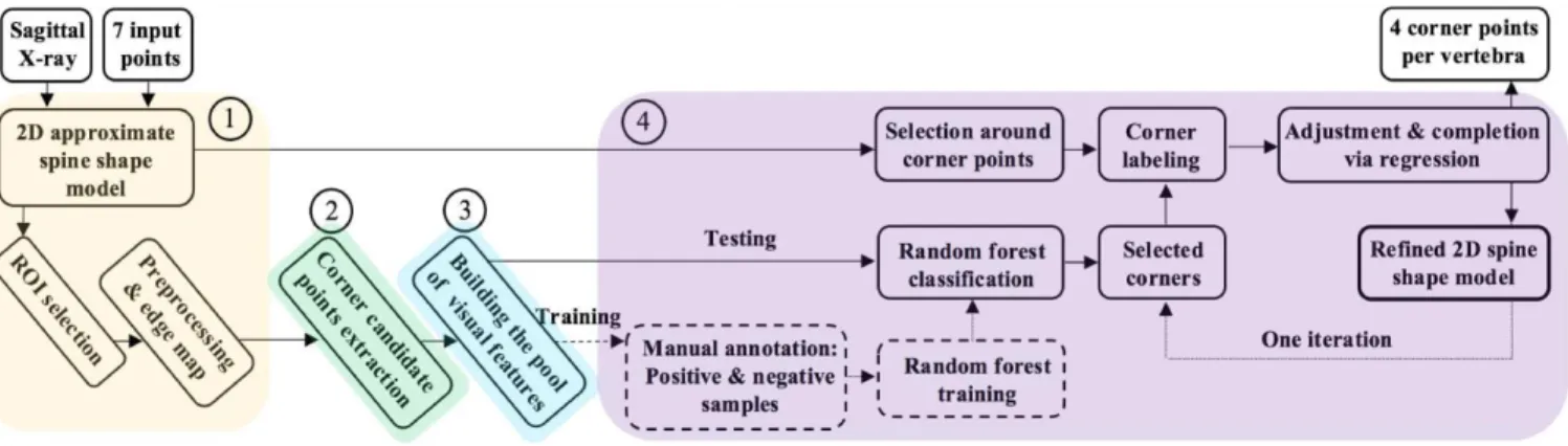
The image processing pipeline, illustrated in Figure 1, consists of the following main steps: (1) preprocessing and edge map computation; (2) identification of corner point candidates; (3) extraction of visual features on candidate points; (4) selection of final corner points with corner-specific Random Forest classifiers trained on a subset of cases, and refinement via regression.
Figure 1 Overall illustration of the work flow, taking as an input a sagittal X-ray image and providing as an output the refined 2D spine shape model.
2.1. Data
2.1.1. Image Dataset
• Our database is composed of 109 subjects (age from 6 to 69 years old), with one sagittal X-ray acquired with an EOS ultra-low dose system (EOS imaging, Paris, France), and collected from various hospitals and research centres. The database is a clinical cohort, acquired in the context of standard clinical diagnosis and treatment planning, and was obtained within a protocol approved by ethical committees of the centres with written consent from the patients.
• Pixel size varies between 0.17940.1794 mm2 and 0.18320.1832 mm2. The Field of view (FOV)
includes the superior tip of the odontoid bone, all cervical (C1 to C7), thoracic (T1 to T12) and lumbar (L1 to L5) vertebrae and the superior endplate of the sacrum bone.
• The population includes asymptomatic and scoliotic spines with characteristics and compositions detailed in Table 1.
Table 1
Training and testing datasets characteristics
Number of cases
Age (year)
Cobb angle (∘)
female male total
range
mean
range
Ave.
Asymptomatic
set
Group_A1
16
15
31
19-60
26
-
-
Group_A2
3
3
6
11-35
26
-
-
Group_A3
6
10
16
49-69
55
-
-
Scoliotic
set
Group_S1
4
1
5
11-17
13
9 - 16
12.8
Group_S2
20
4
24
6-17
13
21.8 - 93
51
Group_S3
8
1
9
10-13
12
7.1 - 19.7
14.6
Group_S4
18
-
18
11-17
13
21.7 - 71.9
38.1
2.1.2. Initialization with a 2D Spine Shape Model
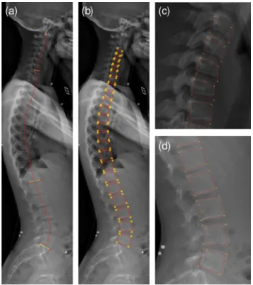
Surgeons willing to perform quantitative radiographic measures on biplanar X-rays for surgical planning have currently two options: positioning and manually correcting a full 2D or 3D spine shape model with commercial software tools such as sterEOS from EOS imaging or manually extracting a subset of localized geometric features as with the Surgimap Spine software tool (Lafage et al., 2015). Academic groups are actively working on improving the robustness and precision of 3D spine shape model reconstruction from X-rays (Humbert et al., 2009; Korez et al., 2016; Zhang et al., 2013), but have not yet reached fully-automated solutions that are precise enough. Even full-automation of the extraction of the spinal curve on X-rays remains challenging for scoliotic cases (Duong et al., 2010). In this context, we exploit an in-house 2D shape model (Humbert et al., 2009) positioning to initialize our processing pipeline. For each sagittal radiograph, an operator first defines seven points (Figure 2(a)), used to position the superior sacrum endplate, T12 inferior and C7 superior endplates, and the tip of the odontoid bone, which sets the upper limit of the spine. This information, which takes less than 1 minute to enter, is sufficient to draw an approximate mid-line of the vertebral bodies. Inspired from the work presented in (Humbert et al., 2009), a 2D model of the spine is built (Figure 2(b)), inferring the size and location of all vertebral endplates via multilinear regression. This
2D model provides approximate positions of vertebral corners that are later refined with the proposed processing pipeline.
Figure 2 (a) Sacrum endplate, T12 inferior and C7 superior endplates along with odontoid are first manually annotated, from which the 2D approximate spine shape model in (b) is computed. (c) and (d) depict the spine shape model in cervical and lumbar regions.
We use this initial 2D spine shape model to define two regions of interest (ROIs): The cervical region (from C3 to C7), and the lumbar region (from L1 to L5) which are processed separately
2.2. Image Preprocessing
First, the lumbar ROI is downsampled by a factor of two. This operation increases homogeneity of the structures, decreases matrix sizes (hence computational complexity) and homogenizes sizes of vertebral structures in pixels, since lumbar vertebrae are almost twice as big as cervical vertebrae.
Images are denoised using a 55 Wiener filter (with a noise variance parameter inferred via averaging local estimated variances), and then enhanced using a median filter, making the interior parts of the vertebrae more homogeneous while maintaining the contrast at the vertebral borders. We then use the contrast limited adaptive histogram equalization (CLAHE) method (Zuiderveld, 1994) to locally improve contrast and attenuate intensity variations across the field of view (due, for example, to varying thickness of surrounding tissues). Finally we generate an edge map using the Canny edge detector (Canny, 1986).
2.3. Corner Point Candidate Extraction
Following the method and parameters described in the study of (Ebrahimi et al., 2016), we convert the edge map into a set of connected edge segments using the polyline simplification method introduced in (Douglas
and Peuker, 1973) and discard points placed along flat edges. This leads to a subset of edge points that are considered as corner point candidates (magenta points in Figure 7(f&g)).
2.3.1. Definition of Vertebral Geometric Features and Ground-Truth
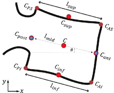
As illustrated in Figure 3, four corner types are defined: (1) anterior superior (AS), (2) anterior inferior (AI), (3) posterior inferior (PI), and (4) posterior superior (PS).
Figure 3 Geometric features measured per vertebra: corner points (CAS, CAI, CPI, and CPS), endplate lengths (lsup, linf), endplate centers (Csup, Cinf), posterior and anterior wall centers (Cpost, Cant), midline connecting the two wall centers (lmid), vertebra orientation θ with
respect to the horizontal image axis, and centre point C.
Regarding the length and orientation, if 𝑐1 and 𝑐2 are two corners defining the two ends of an endplate, the endplate length (𝐿) and orientation (𝐴) are computed as below:
𝐿 = √(𝑥𝑐2− 𝑥𝑐1)2+ (𝑦𝑐2− 𝑦𝑐1)2, (1)
𝐴 = 𝑎𝑟𝑐𝑡𝑎𝑛 (𝑦𝑐2− 𝑦𝑐1 𝑥𝑐2− 𝑥𝑐1
). (2)
To define our ground-truth and generate a training set for the RF classifiers, we manually labelled the candidate points selected from the edge map as either AS, AI, PI, PS corner type or non-corner. To facilitate the manual annotation procedure and handle the large uncertainty in manual selection of corner candidates, the operator was asked to click candidate corner points on the original radiograph, visualizing the candidate points selected from the edge map. The operation was repeated separately for each corner type. All candidate points within manual uncertainty range of 1.4 mm, as well as the clicked point were preserved as instances of the desired corner class. The operator added corner points at regions where no
candidate was present. This might happen in case of noise, occlusion, and poor contrast at corner regions that affect the edge map quality from which the candidates are obtained.
2.4. Visual Features Extraction
We extract three types of visual features (HOG, Haar-like features, and contextual features) which are detailed below.
2.4.1. HOG Features
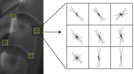
Histograms of oriented gradients (HOG) were introduced in (Dalal and Triggs, 2005). We use square patches of size 1515 pixels centred on each of the candidate points. Patches are divided into 33 cells, and histograms use 12 orientation bins. This leads to a HOG feature vector of length 108 (=129), for each candidate point. Figure 4 shows the assembly of HOG features positioned at corners of a cervical vertebra.
Figure 4 HOG features computed for the corners of a cervical vertebra.
2.4.2. Haar-Like Features
Two features based on Haar-like filtering were introduced in (Ebrahimi et al., 2016). In the current study, we add 16 Haar-like features, to improve sensitivity to corner orientation and local appearance.
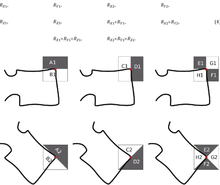
The responses computed from the Haar-like filters (Figure 5) are defined in Equation 3. They are recorded via centring the filters on each candidate point.
𝑅𝑋1= 𝐵1− 𝐴1,
𝑅𝑌1= 𝐶1− 𝐷1,
𝑅𝑋2= 𝐵2− 𝐴2, 𝑅𝑌2= 𝐶2− 𝐷2,
𝑅𝑍1= (𝐺1+ 𝐻1) − (𝐸1+ 𝐹1), 𝑅𝑍2= (𝐺2+ 𝐻2) − (𝐸2+ 𝐹2)
Multiple filter scales are used to handle variability in vertebrae shapes and orientations, corresponding to filters of size: 1919, 1515, and 1111 pixels. From the filter responses, we define the following set of 10 features:
𝑅𝑋1, 𝑅𝑌1, 𝑅𝑋2, 𝑅𝑌2,
(4)
𝑅𝑍1, 𝑅𝑍2, 𝑅𝑋1𝑅𝑌1, 𝑅𝑋2𝑅𝑌2,
𝑅𝑋1𝑅𝑌1𝑅𝑍1, 𝑅𝑋2𝑅𝑌2𝑅𝑍2.
Figure 5 Definition of the n×n Haar-like filters (black = −1, white = 1). The filter size n varies with the scale of the filter. The upper row set of filters targets 0° oriented corners and the lower row targets 45° oriented corners.
The maximum response over all scales is retained for each feature value. 𝑅𝑋1, 𝑅𝑌1, 𝑅𝑋2, 𝑅𝑌2 are edge features which encode local appearance and contrast around the points of interest.
(𝑅𝑋1𝑅𝑌1, 𝑅𝑍1) and (𝑅𝑋2𝑅𝑌2, 𝑅𝑍2) are corner appearance features with high values at corners with 0 and 45 orientations respectively.
(𝑅𝑋1𝑅𝑌1 𝑅𝑍1) and (𝑅𝑋2𝑅𝑌2𝑅𝑍2) are corner appearance & type features, which return high values at corners and encode corner type (concave versus convex) with their sign. The following five additional Haar-like features are extracted:
𝑂1= 𝑅𝑋1− 𝑅𝑋2, 𝑂2= 𝑅𝑌1− 𝑅𝑌2,
(5)
𝑂3 = (𝑅𝑋1𝑅𝑌1) − (𝑅𝑋2𝑅𝑌2), 𝑂4= 𝑅𝑍1− 𝑅𝑍2,
𝑂5 = (𝑅𝑋1𝑅𝑌1𝑅𝑍1) − (𝑅𝑋2𝑅𝑌2𝑅𝑍2).
These features are based on subtractions of edge and corner features computed at 0 and 45 orientations. The feature values are largest for 0 and 45 oriented corners (either positive or negative signs) and smallest for corners oriented at ±22.5. These features, therefore, refine the encoding of the corner orientation.
One last feature is computed as the local average intensity at each candidate point (filter size 1515 pixels). We end-up with a 16-dimensional Haar-like feature vector.
2.4.3. Contextual Features
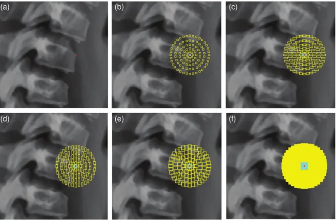
Figure 6 Contextual features. (a) A candidate corner point (in red); (b) Arrangement of 3×3 contextual patches around candidate point within the cyan central patch; (c)-(e) 3×7, 7×3, 7×7 contextual patches; (f) All 36 different contextual patches, which leads to a very
dense sampling over the candidate point's neighbourhood.
We include a novel configuration of contextual features to capture visual characteristics (intensity and contrast) of neighbouring structures, which enable us to add robustness in the identification of corners and their types. Contextual features are also exploited in (Al Arif et al., 2017; Glocker et al., 2013, 2012) with different formulations. As illustrated in Figure 6, we define a large set of contextual patches around each candidate point as follows. Patch height and width take every possible combination of the following values: {3, 5, 7, 9, 11, 13} pixels. Patches are created with any dimension and shifted away from the candidate point position by forming a circle of regularly-positioned patches at distances of {6, 12, 19, 27, 36} pixels. In our implementation, a total number of 3,636 contextual patches is considered for each candidate point. To accelerate pixel summations over all subregions encompassed by the aforementioned patches we use the integral image of (Viola and Jones, 2004), which provides the outcome with just three sum operations.
We generate two sets of contextual features at each candidate point for every size of contextual patches: (1) the average intensity value inside each contextual patch, and (2) the difference between average intensities inside the central patch and its corresponding contextual patches.
Overall, 7,236 (3,636 type (1) and 3,600 type (2)) contextual features are computed for each candidate point.
2.5. Random Forest Training
We train corner-specific random-forest (RF) classifiers (Breiman, 2001) separately for lumbar and cervical spine regions. For both regions, we train four RF classifiers to predict the four corner types of each vertebra. We work with forests of 500 trees, where the standard Gini metric is applied for node splitting. Maximum depth per tree is controlled by the minimum number of observations per branch node, which is set to 10. The minimum number of observations per tree leaf is set to one, and the maximum number of splits is defined to be 𝑚 − 1, where 𝑚 corresponds to the number of observations. Among the pool of 𝑁𝑓 = 7,360 features per sample point, we randomly select √𝑁𝑓 86 features at each split node. The RF outcome label corresponds to the class having the majority of votes over the ensemble of decision trees.
The training set includes Group_A1 and Group_S1-S2 (cf. Section 2.1), with 𝑁 = 60 asymptomatic or scoliotic subjects that cover a wide variety of vertebrae shapes and orientations.
For a corner type, positive training samples are all the manually annotated points, while the negative samples are the other three corner types plus a random selection of 10% of the non-corner points.
The testing set consists of Group_A2-A3 and Group_S3-S4 (cf. Table 1), forming a cohort of 𝑁 = 49 subjects, categorized into three groups G that differ in age and disease severity. G1 = Group_A2 + Group_S3 (N=15) is composed of adolescents and young subjects with no or moderate scoliosis. In G2 = Group_S4 (N=18) we have severe AIS patients. Finally, in G3 = Group_A3 (N=16) we gather non-scoliotic adults and older subjects, who mainly suffer from osteophytes, and cervical deformity.
We illustrate in Figure 7(h) the outcome of a RF classification on all vertebrae, using one colour per corner type. At this stage, several candidate points can be labelled as the same corner point by the RF classifiers, and some corner position might not have any labelled point. We solve these issues with the next and final step.
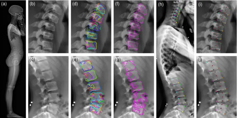
Figure 7 Visual illustrations of the processing steps: (a) Original sagittal X-ray (EOS™); (b-c) Enhanced images in cervical and lumbar regions; (d-e) Simplified edge segments plotted on cervical and lumbar regions; (f-g) Corner point candidates after polyline simplification; (h) Corners coloured by type (green=AS, yellow=AI, magenta=PI, cyan=PS); (i-j) Corners, vertebrae centres, and endplate centres provided by manual selection (red cross) and by the algorithm (black circles).
2.6. Final Adjustment of Corner Points
Local decisions are made in the neighbourhood of the initial corner point positions, exploiting the a priori knowledge given by the approximate 2D shape model of the spine. At this stage, detected corners in the lumbar region are mapped back to the original X-ray image via upscaling of their coordinate by a factor of 2, as they were obtained on downsampled images. We define a circular search area around each approximate corner positions and then preserve the detected points encompassed in the search area. We set the search area radius to 23 pixels, which is approximately half the height of a vertebra. The following processing is then applied:
(1) If there are multiple points labelled at a corner position, their coordinates are averaged to lead to a single corner point.
(2) If there is no point labelled at a corner position, a regression model is used to infer the position of the missing corner based on surrounding corner points, as follows.
We apply the strategy introduced in (Albrecht et al., 2013) that provides a closed-form formula for the conditional distribution of a statistical shape model given partial data. This strategy enables us to estimate the position of the missing corner points given the localized ones. The model uses an uncertainty parameter on corner coordinates which was set to 10 pixels in our work. The regression step is based on a generic statistical position model built with the manually annotated corner points from the training set. For each subject, the 2D coordinates of the four corner points of vertebrae C3 to C7 and L1 to L5 are extracted. We express coordinates in a frame where the odontoid summit, manually identified earlier, is the origin, and
the 𝑋 and 𝑌 axis are the natural image axis. The coordinates are concatenated in a line vector, and a principal component analysis (PCA) is applied to each region individually, computing the mean model 𝜇 and the principal components 𝑄 (eigenvectors of the 50 largest eigenvalues of the covariance matrix). This framework enables us to infer a missing corner position (2D coordinates) by adding to the mean model a linear combination of its principle components according to the formula 𝜇 + 𝑄𝛼. The closed formula for 𝛼 is given in (Albrecht et al., 2013).
The regression model is used twice in our algorithm. The first run updates the search area where we collect corner points detected by RF classifiers. The second run enables to fill the remaining missing corners. From the four corners of a vertebra we are capable to extract the following vertebral geometric features: Vertebra centre, superior and inferior endplate lengths and centres, and vertebra orientation (Figure 3). 3. Results
We first test the performance of the RF classifiers when trained with individual feature types (CF, HOG, or Haar) or the combination of the three types (All). We report in Table 2 sensitivity and precision measures of corners detected within a radius of 1.4 mm from the manually-selected ground truth positions. Obtained from the work (Ebrahimi et al., 2016), this radius value corresponds to the uncertainty on the manual identification of corner points. Detection performance is reported on corner points detected by RF classifiers but not adjusted with the final shape model regression. We observe that precision with the combination of features performs best for both regions. Sensitivity with only Haar features is the highest, but is systematically associated with poorest precision. It also appears that CF features contribute to a great improvement of the precision in the lumbar region, performing almost as well when used as single feature type than when combined. But, overall, combining the three feature types improves precision while slightly decreasing sensitivity compared to the Haar features when used alone. Visual inspection also confirmed that the three feature types complement each other’s for challenging corners when one individual type returns a weak response. Regarding computation time for these features, each spine region contains between 400 and 800 candidate points after edge extraction and simplification. Feature extraction on 800 candidate points takes about 0.5 seconds for Haar, 7 seconds for HOG, and 7 seconds for CF. when implemented without specific optimization in Matlab© and running on a PC with a 2.4GHz processor and 8Gb of RAM. Given the complementarity of these features and the low computational times, we choose to work with the combination of the three. The overall computational pipeline with this combination takes less than 2 minutes to process the 10 vertebrae (C3-C7 and L1-L5).
Table 2
Performance of RF classifiers with different feature types,
reported for corner detection within the confidence interval. (CF:
Contextual Features, HOG: Histograms of Orientated Gradients,
Haar: Haar-like features, All=combination of the 3 feature types)
Region
All
CF
HOG
Haar
Cervical
Sensitivity
81%
81%
81%
82%
Precision
88%
86%
83%
77%
Lumbar
Sensitivity
67%
66%
54%
72%
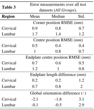
Table 3
Error measurements over all test
datasets (All Groups).
Region
Mean
Median
Std.
Corner position RMSE (mm)
Cervical
0.9
0.8
0.7
Lumbar
1.7
1.4
1.2
Centre position RMSE (mm)
Cervical
0.5
0.4
0.4
Lumbar
1
0.8
0.7
Endplate centre position RMSE (mm)
Cervical
0.7
0.6
0.5
Lumbar
1.2
1
0.8
Endplate length difference (mm)
Cervical
0.2
0.2
1.2
Lumbar
0.7
0.8
2
Global orientation difference (∘)
Cervical
-2.1
-1.8
3.1
Lumbar
-0.1
-0.5
2.9
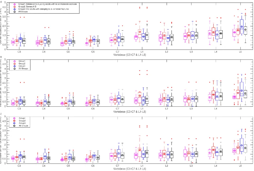
To assess the precision of our framework, we then compare the outcome of our proposed method with the gold standard, obtained manually by an expert. Average localization root-mean square errors (RMSE) are computed for corner positions, vertebrae centres, and vertebrae endplate centres. The reported error value for the vertebra endplate centre is the average over the superior and inferior endplate centres. The endplate length signed differences between the ground truth and the algorithm outcome, as well as, the vertebra orientation signed differences are also reported. A summary of the computed errors for all three groups is provided in Table 3. Population statistics for these five error measures are further detailed in Figure 8 and Figure 9, distinguishing the following subgroups of subjects:
• G1 (N=15): Adolescents and young adults with no or moderate scoliosis. Used as the reference group; • G2 (N=18): Severe AIS;
• G3 (N=16): Old adults.
A Wilcoxon signed-rank test was performed to assess possible statistical significant differences of errors between the reference group (G1) and the diseased groups (G2 and G3). This test was run grouping measures from C3-C7 and from L1-L5 (hence two tests per error measurement).
Results in Table 3 show that RMSE positions errors and length differences are always smaller in the cervical than in the lumbar region, but median values all remain within the manual uncertainty range of 1.4 mm. On the other hand, orientation differences are larger in the cervical region. As depicted in Figure 8, the lowest average localization errors are achieved on the reference group G1. Lowest mean ± Std corner
localization errors are equal to 0.8 ± 0.5 mm (cervical region in G1) and 1.5 ± 1.1 mm (lumbar region in G1). Highest mean ± Std corner localization errors are equal to 1.1 ± 0.9 mm (cervical region in G3) and 1.8 ± 1.3 mm (lumbar region in G2). With respect to vertebrae centre localization errors, all mean ± Std. values are below 1 ± 0.5 mm except for lumbar spine in G2 and G3 where it reaches 1.1 ± 0.8 mm. Endplates and vertebrae centre localization errors show very similar patterns in terms of ranges of values and evolutions of error distributions across spine levels.
Regarding endplate length differences in Figure 9(a), group-means (bias) are all below 0.2 mm in the cervical region while they reach 1.1 mm in the lumbar spine, with the G1 group showing sometimes larger errors than G2 or G3. Overall, spreads of errors then to be larger in the lumbar region. As for orientation differences (Figure 9(b)), G1 has the smallest values both in the lumbar and cervical spine, with respective values of −0.4 ± 2.3 and −1.4 ± 2.8 while highest values are found in G2 and G3, reaching −1.6 ± 3.6 in the cervical spine in G3. Among all vertebrae, L1-L3 exhibit the smallest error levels and ranges, for all groups. Overall, we observe a trend of larger errors in the lumbar region for point localization and length measurements and of smaller errors for orientation measures in L1-L3.
The Wilcoxon signed-rank test showed no significant differences of error measures between the reference group and the two disease groups (p=0.001) for all measures except two: cervical corners and endplate centres localization errors of G1 versus G3.
Finally, few outliers (up to 4 per vertebra) appear for some measures, and correspond to cases with strong visual ambiguity regarding the corner shape.
4. Discussion and Conclusion
A novel processing pipeline for the task of vertebrae corner detection on sagittal X-rays is presented which provides an efficient compromise between computational time and accuracy. The proposed framework is based on initial information that requires minimal user input, taking less than 1 minute to complete. Indeed, only seven “clicks” are needed to define three vertebral endplates and the top of the odontoid. From that, an approximate spine shape model is built for ROI selection, and an accurate localization of corners is tackled by the proposed image processing and statistical modelling pipeline. Most existing works on vertebrae corner detection reported only corner detection rate without analysing the accuracy of the corner positions. Compared to previously published semi-automated methods for vertebrae corner and orientation measurements, listed in Table 4, this study provides a more extensive evaluation, reporting errors corner localization, derived end-plate positions and orientations. Moreover, our study encompasses results on both cervical and lumbar vertebrae, while most of the advanced methods toward automation of vertebrae corner detection from X-rays have been evaluated on only one of these two regions.
Figure 8 RMSE localization errors per vertebra computed for individual test groups and all combined together: (a) Corner localization errors; (b) Localization errors of vertebrae centres; (c) Localization errors of endplate centres (average errors of upper and lower endplates). Circles in the box plots indicate the mean values. On each box, horizontal lines indicate 25%, 50% and 75% percentiles. The two upper and lower whiskers (dotted lines) show the confidence interval (critical value at 99.3%). The red +
Figure 9 (a) Endplate length differences. The value is measured by averaging the differences over the upper and lower vertebra endplates; (b) Vertebrae orientation differences. Orientation is defined by the angle between the horizontal axis of the image and the midline connecting the two centres of posterior and anterior vertebrae walls
Table 4
Overview of state of the art approaches for vertebra corner detection on planar X-ray images. NA: Not available, C: Cervical, L: LumbarPublication Manual Input Method Region Pathology
Dataset # (training/testing) cross-validation Localization RMSE Orientation error (Benjelloun et al., 2011) 2 clicks for cervical ROI selection
Harris features+active shape
model C3-C7 NA NHANES II (75/100) NA NA (Lecron et al., 2010) 2 clicks for cervical ROI selection
Polygonal approximation C3-C7 NA NHANES II
(-/NA) NA NA
(Lecron et al., 2012)
2 clicks for cervical ROI selection
SIFT features+SVM classifier C3-C7 NA
NHANES II (49/1) leave-one-out NA NA (Larhmam et al., 2014) 2 clicks for cervical ROI selection GHT+K-means C3-C7 No NHANES II + Hospital (25/66) NA 6.7∘
(Al Arif et al., 2015a) 5 vertebrae
centres Hough Forest C3-C7 Yes
(96/10)
10-fold 4.41 ± 4.14 mm NA (Al Arif et al., 2015b) 5 vertebrae
centres
Hough Forest+Haar like
features C3-C7 Yes
(80/10)
10-fold 3.03 ± 3.08 mm NA (Ebrahimi et al., 2016) 1 point click as
reference
Haar-like
features+Thresholding L1-L5 Yes
Hospital(s)
(-/21) 1.2 ± 0.8 mm NA
(Al Arif et al., 2017) 5 vertebrae centres
1. Intensity and gradient 2. Haar-like features 3. Random mirrored features 4. CNN features
5. Structured forest features
C3-C7 Yes Features (1-5): (80/10) 10-fold Feature (6): (80/10) leave-one-out
Best result for: Haar-like features mean= 2.01 mm
6. multi scale Harris corner detection
Proposed method 7 point clicks for 2D shape model
Haar-like+HOG+CF
features+Random Forest C3-C7 & L1-L5 Yes
5 Hospitals (60/49) C: 0.9 ± 0.7 mm L: 1.7 ± 1.2 mm C: -2.1∘ ± 3.1∘ L: 1.7∘ ± 1.2∘
Among the literature that focuses on vertebrae corner detection and reports detection precision, (Al Arif et al., 2017, 2015a, 2015b) provided these values on the cervical region (C3-C7). In (Al Arif et al., 2015b) they reported average RMSE values of 3.033.08 mm. In (Al Arif et al., 2017), a mean corner localization error of 2.01 mm is reported using a Hough forest classifier with mixed intensity and contrast Haar-like features and a rectangular ROI. In (Ebrahimi et al., 2016) an RMSE error of 1.20.8 mm on lumbar posterior corners was reported. In this work, using the same metrics, we obtained average corner localization RMSE values of 0.90.7 mm for the cervical region, and 1.71.2 mm for the lumbar region. Our results agree with Al Arif’s observation of a slight increase in average corner localization errors from C3 to C7.
Regarding the spine orientation (Larhmam et al., 2014) reported an average RMSE of 6.7 for cervical vertebrae (C3-C7 with min = 5.55 & max = 8.22). In this study, we report a mean (bias) ± Std. for orientation differences of −0.1 ± 2.9 in the lumbar region, and −2.1 ± 3.1 in the cervical region.
Variability of manual landmark localization at each vertebral level was evaluated in (Champain et al., 2006) but on shape parameters different that the ones evaluated in our study. However, it seems that our orientation errors are slightly higher than manual uncertainty in asymptomatic subjects, while in pathologic cases they are similar. A major contribution of our proposed methodology is the design of our pool of image features, composed of three complementary types. HOG features have proven their efficiency in encoding robust local visual characteristics. The tailored Haar-like features provide specific discriminative power for corner detection and determining the corner types, however, their spatial range is limited. Adding some contextual features lets us explore large neighbouring regions around the candidate points, which leads to a reinforced discrimination against false positives. Reported results show that the combination of these three feature types improves the precision of the detected corner positions. To the best of our knowledge, the proposed contextual feature design has not been explored for corner detection in previous work. Although the pool of features is very large, its generation is not computationally demanding. Choosing random forest classifiers for learning the characteristics of the corner points while mixing asymptomatic and pathologic subjects in the training set was shown to work efficiently with limited computational efforts and parameter tuning. Another original contribution is the design of an iterative process, combining image processing and statistical shape modelling. Indeed, corner identification is facilitated with properly defined search areas. Then, using a first set of detected corners, the statistical shape model is refined, which yields updated search areas for undetected corners, thus facilitating additional detection.
Results show best overall performance for the test group with asymptomatic or moderate AIS (G1). This was expected as deformities of the spines are minimal, and consequently there exists less ambiguity at corner regions. In the group of severe AIS subjects (G2), we deal with highly deformed spines in the lumbar region. This causes superimposition of bone signal at the corner areas, and affects the algorithm precision. In such group, even the reproducibility of manual annotations considerably decreases. However, in contrast with the thoracolumbar region, the spine deformities in the cervical spine remain limited, and in this region our results are similar to those in G1. Non-scoliotic old patients (G3) have osteophytes and cervical deformities. As a result, in the cervical region we observe the largest average error differences when comparing to G1, while in the lumbar region average error levels are comparable. This also might be the consequence of not including any old subject in our training dataset. Despite smaller localization errors in the cervical region, orientation errors are higher in this region, likely due to the smaller size of cervical vertebrae. Focusing on mean orientation differences, in relation with a possible bias, values are −2.1 in the cervical spine, and closer to 0 (−0.1) in the lumbar region. Higher bias in the cervical region may be due to corner shape ambiguities and probable pathologies such as osteophytes. In practice, since the bias represents
a systematic error, this issue could be addressed by adding a potential post-correction of the cervical corner positions with respect to the known orientation bias.
Overall, the performance of our proposed method compares favourably to previously published approaches in terms of precision and level of manual supervision. Nevertheless, our method has two main limitations. First, the thoracic part was not investigated, since the visual quality of sagittal X-rays in this region is lower, and since the major interest for clinical analysis is on lumbar and cervical spine regions. However, with the output refined shape models of the lumbar and cervical regions, the applied regression algorithm recalculates the position of model’s elements on the thoracic region as well, leading to a potential global improvement of the model precision which will be evaluated in a future study. The second limitation is that the precision of the localized corners, especially in asymptomatic or moderately scoliotic subjects, can be lower than reported by methods exploiting more manual supervision. Extension of the method could consider adding a level of confidence to the detected corners, so that the user is pointed to corners that need manual verification and correction.
This study is the first step toward a universal solution for fast and extensive shape modelling of the whole spine on sagittal X-rays. Extension to the thoracic region will require a dedicated image enhancement pre-processing. Automated localization of additional spine bone landmarks, such as pedicles and spinous processes, constitutes ongoing efforts from our group. Preliminary results confirm that the combination of the three visual features is beneficial over a single type when using a random forest classifier for the detection, in particular the HOG type being critical for pedicles detection.
Acknowledgments
The authors are grateful to the ParisTech BiomecAM chair program on subject-specific musculoskeletal modelling for funding, and particularly Société Générale and COVEA.
References
Al Arif, S.M.M.R., Asad, M., Gundry, M., Knapp, K., Slabaugh, G., 2017. Patch-based corner detection for cervical
ss. Image Commun.
Al Arif, S.M.M.R., Asad, M., Knapp, K., Gundry, M., Slabaugh, G., 2015a. Hough Forest-based Corner Detection for Cervical Spine Radiographs, in: 19th Conference on Medical Image Understanding and Analysis. Lincoln, UK.
Al Arif, S.M.M.R., Asad, M., Knapp, K., Gundry, M., Slabaugh, G., 2015b. Cervical vertebral corner detection using haar-like features and modified hough forest, in: 5th IEEE International Conference on Image Processing Theory, Tools and Applications (IPTA). Orleans, France.
Albrecht, T., Lüthi, M., Gerig, T., Vetter, T., 2013. Posterior shape models. Med. Image Anal. 17, 959–973. Amabile, C., Le Huec, J.C., Skalli, W., 2016. Invariance of head-pelvis alignment and compensatory
mechanisms for asymptomatic adults older than 49 years. Eur. Spine J. 1–9.
Benjelloun, M., Mahmoudi, S., Lecron, F., 2011. A framework of vertebra segmentation using the active shape model-based approach. Int. J. Biomed. Imaging 2011, 1–14.
Boissiere, L., Takemoto, M., Bourghli, A., Vital, J.M., Pellise, F., Alanay, A., Yilgor, C., Acaroglu, E., Perez-Grueso, F.J., Kleinstuck, F., Obeid, I., 2017. Global tilt and lumbar lordosis index: two parameters correlating with health-related quality of life scores-but how do they truly impact disability? Spine J. 17, 480–488. Breiman, L., 2001. Random forests. Mach. Learn. 45, 5–32.
Canny, J., 1986. A computational approach to edge detection. IEEE Trans. Pattern Anal. Mach. Intell. 8, 679– 698.
Champain, S., Benchikh, K., Nogier, A., Mazel, C., Guise, J. De, Skalli, W., 2006. Validation of new clinical quantitative analysis software applicable in spine orthopaedic studies. Eur. Spine J. 15, 982–991. Dalal, N., Triggs, B., 2005. Histograms of oriented gradients for human detection, in: Proceedings - 2005 IEEE
Computer Society Conference on Computer Vision and Pattern Recognition, CVPR 2005. Washington, DC, USA, pp. 886–893.
Douglas, D.H., Peuker, T.K., 1973. Algorithms for the reduction of the number of points required to represent a digitized line or its caricature. Cartogr. Int. J. Geogr. Inf. Geovisualization 10, 112–122.
Duong, L., Cheriet, F., Labelle, H., 2010. Automatic Detection of Scoliotic Curves in Posteroanterior Radiographs. IEEE Trans. Biomed. Eng. 57, 1143–1151.
Ebrahimi, S., Angelini, E., Gajny, L., Skalli, W., 2016. Lumbar spine posterior corner detection in X-rays using Haar-based features, in: 13th IEEE International Symposium on Biomedical Imaging (ISBI). Prague, Czech Republic.
Glocker, B., Feulner, J., Criminisi, A., Haynor, D.R., Konukoglu, E., 2012. Automatic localization and identification of vertebrae in arbitrary field-of-view CT scans., in: 15th International Conference on Medical Image Computing and Computer-Assisted Intervention (MICCAI). Nice, France.
Glocker, B., Zikic, D., Konukoglu, E., Haynor, D.R., Criminisi, A., 2013. Vertebrae localization in pathological spine CT via dense classification from sparse annotations, in: 16th International Conference on Medical Image Computing and Computer-Assisted Intervention (MICCAI). Nagoya, Japan.
Harris, C., Stephens, M., 1988. A Combined Corner and Edge Detector, in: 4th Alvey Vision Conference (AVC). Manchester, UK.
Hasegawa, K., Okamoto, M., Hatsushikano, S., Shimoda, H., Ono, M., Watanabe, K., 2016. Normative values of spino-pelvic sagittal alignment, balance, age, and health-related quality of life in a cohort of healthy adult subjects. Eur. Spine J. 25, 3675–3686.
Humbert, L., De Guise, J.A., Aubert, B., Godbout, B., Skalli, W., 2009. 3D reconstruction of the spine from biplanar X-rays using parametric models based on transversal and longitudinal inferences. Med. Eng. Phys. 31, 681–687.
Klinder, T., Ostermann, J., Ehm, M., Franz, A., Kneser, R., Lorenz, C., 2009. Automated model-based vertebra detection, identification, and segmentation in CT images. Med. Image Anal. 13, 471–482.
Korez, R., Aubert, B., Cresson, T., Parent, S., Vrtovec, T., de Guise, J., Kadoury, S., 2016. Sparse and multi-object pose+shape modeling of the three-dimensional scoliotic spine, in: 2016 IEEE 13th International Symposium on Biomedical Imaging (ISBI). IEEE, pp. 225–228.
Lafage, R., Ferrero, E., Henry, J.K., Challier, V., Diebo, B., Liabaud, B., Lafage, V., Schwab, F., 2015. Validation of a new computer-assisted tool to measure spino-pelvic parameters. Spine J. 15, 2493–2502.
Larhmam, M.A., Benjelloun, M., Mahmoudi, S., 2014. Vertebra identification using template matching modelmp and K-means clustering. Int. J. Comput. Assist. Radiol. Surg. 9, 177–187.
Lecron, F., Benjelloun, M., Mahmoudi, S., 2012. Fully Automatic Vertebra Detection in X-Ray Images Based on Multi-Class SVM, in: SPIE Medical Imaging: Image Processing. San Diego, USA.
Lecron, F., Benjelloun, M., Mahmoudi, S., 2010. Points of interest detection in cervical spine radiographs by polygonal approximation, in: 2nd International Conference on Image Processing Theory, Tools and Applications (IPTA). Paris, France.
Lim, P.H., Bagci, U., Bai, L., 2013. Introducing Willmore Flow Into Level Set Segmentation of Spinal Vertebrae. IEEE Trans. Biomed. Eng. 60, 115–122.
Lowe, D.G., 2004. Distinctive Image Features from Scale-Invariant Keypoints. Int. J. Comput. Vis. 60, 91–110. Neubert, A., Fripp, J., Engstrom, C., Schwarz, R., Lauer, L., Salvado, O., Crozier, S., 2012. Automated detection, 3D segmentation and analysis of high resolution spine MR images using statistical shape models. Phys. Med. Biol. 57, 8357–8376.
Tournier, C., Aunoble, S., Le Huec, J.C., Lemaire, J.P., Tropiano, P., Lafage, V., Skalli, W., 2007. Total disc arthroplasty: Consequences for sagittal balance and lumbar spine movement. Eur. Spine J. 16, 411–421. Viola, P., Jones, M.J., 2004. Robust real-time face detection. Int. J. Comput. Vis. 57, 137–154.
Yao, J., Burns, J.E., Forsberg, D., Seitel, A., Rasoulian, A., Abolmaesumi, P., Hammernik, K., Urschler, M., Ibragimov, B., Korez, R., Vrtovec, T., Castro-Mateos, I., Pozo, J.M., Frangi, A.F., Summers, R.M., Li, S., 2016. A multi-center milestone study of clinical vertebral CT segmentation. Comput. Med. Imaging Graph. 49, 16–28.
Zhang, J., Lv, L., Shi, X., Wang, Y., Guo, F., Zhang, Y., Li, H., 2013. 3-D reconstruction of the spine from biplanar radiographs based on contour matching using the hough transform. IEEE Trans. Biomed. Eng. 60, 1954– 1964.
Zuiderveld, K., 1994. Contrast Limited Adaptive Histogram Equalization, in: Graphics Gems IV. Academic Press Professional, San Diego, USA, pp. 474–485.