PAPER
Characterization of the LIGO detectors during their
sixth science run
To cite this article: J Aasi et al 2015 Class. Quantum Grav. 32 115012
View the article online for updates and enhancements.
Related content
The characterization of Virgo data and its impact on gravitational-wave searches
-LIGO: the Laser Interferometer Gravitational-Wave Observatory
-Reducing the effect of seismic noise in LIGO searches by targeted veto generation
-Recent citations
Gravitational-wave inference in the catalog era: Evolving priors and marginal events Shanika Galaudage et al
-Robust machine learning algorithm to search for continuous gravitational waves Joe Bayley et al
-Dynamic normalization for compact binary coalescence searches in non-stationary noise
S Mozzon et al
Characterization of the LIGO detectors
during their sixth science run
J Aasi
1, J Abadie
1, B P Abbott
1, R Abbott
1, T Abbott
2,
M R Abernathy
1, T Accadia
3, F Acernese
4,5, C Adams
6,
T Adams
7, R X Adhikari
1, C Affeldt
8, M Agathos
9,
N Aggarwal
10, O D Aguiar
11, P Ajith
1, B Allen
8,12,13,
A Allocca
14,15, E Amador Ceron
12, D Amariutei
16,
R A Anderson
1, S B Anderson
1, W G Anderson
12, K Arai
1,
M C Araya
1, C Arceneaux
17, J Areeda
18, S Ast
13, S M Aston
6,
P Astone
19, P Aufmuth
13, C Aulbert
8, L Austin
1, B E Aylott
20,
S Babak
21, P T Baker
22, G Ballardin
23, S W Ballmer
24,
J C Barayoga
1, D Barker
25, S H Barnum
10, F Barone
4,5,
B Barr
26, L Barsotti
10, M Barsuglia
27, M A Barton
25, I Bartos
28,
R Bassiri
29,26, A Basti
14,30, J Batch
25, J Bauchrowitz
8,
Th S Bauer
9, M Bebronne
3, B Behnke
21, M Bejger
31,
M G Beker
9, A S Bell
26, C Bell
26, I Belopolski
28, G Bergmann
8,
J M Berliner
25, A Bertolini
9, D Bessis
32, J Betzwieser
6,
P T Beyersdorf
33, T Bhadbhade
29, I A Bilenko
34,
G Billingsley
1, J Birch
6, M Bitossi
14, M A Bizouard
35,
E Black
1, J K Blackburn
1, L Blackburn
36, D Blair
37, M Blom
9,
O Bock
8, T P Bodiya
10, M Boer
38, C Bogan
8, C Bond
20,
F Bondu
39, L Bonelli
14,30, R Bonnand
40, R Bork
1, M Born
8,
S Bose
41, L Bosi
42, J Bowers
2, C Bradaschia
14, P R Brady
12,
V B Braginsky
34, M Branchesi
43,44, C A Brannen
41,
J E Brau
45, J Breyer
8, T Briant
46, D O Bridges
6, A Brillet
38,
M Brinkmann
8, V Brisson
35, M Britzger
8, A F Brooks
1,
D A Brown
24, D D Brown
20, F Brückner
20, T Bulik
47,
H J Bulten
9,48, A Buonanno
49, D Buskulic
3, C Buy
27,
R L Byer
29, L Cadonati
50, G Cagnoli
40, J Calderón Bustillo
51,
E Calloni
4,52, J B Camp
36, P Campsie
26, K C Cannon
53,
B Canuel
23, J Cao
54, C D Capano
49, F Carbognani
23,
L Carbone
20, S Caride
55, A Castiglia
56, S Caudill
12,
M Cavagliá
17, F Cavalier
35, R Cavalieri
23, G Cella
14,
C Cepeda
1, E Cesarini
57, R Chakraborty
1,
T Chalermsongsak
1, S Chao
58, P Charlton
59,
E Chassande-Mottin
27, X Chen
37, Y Chen
60, A Chincarini
61,
A Chiummo
23, H S Cho
62, J Chow
63, N Christensen
64,
Q Chu
37, S S Y Chua
63, S Chung
37, G Ciani
16, F Clara
25,
D E Clark
29, J A Clark
50, F Cleva
38, E Coccia
65,66,
P-F Cohadon
46, A Colla
19,67, M Colombini
42,
M Constancio Jr
11, A Conte
19,67, R Conte
68, D Cook
25,
T R Corbitt
2, M Cordier
33, N Cornish
22, A Corsi
69,
C A Costa
11, M W Coughlin
70, J-P Coulon
38, S Countryman
28,
P Couvares
24, D M Coward
37, M Cowart
6, D C Coyne
1,
K Craig
26, J D E Creighton
12, T D Creighton
32, S G Crowder
71,
A Cumming
26, L Cunningham
26, E Cuoco
23, K Dahl
8,
T Dal Canton
8, M Damjanic
8, S L Danilishin
37, S D
’Antonio
57,
K Danzmann
8,13, V Dattilo
23, B Daudert
1, H Daveloza
32,
M Davier
35, G S Davies
26, E J Daw
72, R Day
23, T Dayanga
41,
G Debreczeni
73, J Degallaix
40, E Deleeuw
16, S Deléglise
46,
W Del Pozzo
9, T Denker
8, T Dent
8, H Dereli
38, V Dergachev
1,
R De Rosa
4,52, R T DeRosa
2, R DeSalvo
68, S Dhurandhar
74,
M Dí az
32, A Dietz
17, L Di Fiore
4, A Di Lieto
14,30, I Di Palma
8,
A Di Virgilio
14, K Dmitry
34, F Donovan
10, K L Dooley
8,
S Doravari
6, M Drago
75,76, R W P Drever
77, J C Driggers
1,
Z Du
54, J-C Dumas
37, S Dwyer
25, T Eberle
8, M Edwards
7,
A Ef
fler
2, P Ehrens
1, J Eichholz
16, S S Eikenberry
16,
G Endröczi
73, R Essick
10, T Etzel
1, K Evans
26, M Evans
10,
T Evans
6, M Factourovich
28, V Fafone
57,66, S Fairhurst
7,
Q Fang
37, B Farr
78, W Farr
78, M Favata
79, D Fazi
78,
H Fehrmann
8, D Feldbaum
16,6, I Ferrante
14,30, F Ferrini
23,
F Fidecaro
14,30, L S Finn
80, I Fiori
23, R Fisher
24, R Flaminio
40,
E Foley
18, S Foley
10, E Forsi
6, L A Forte
4, N Fotopoulos
1,
J-D Fournier
38, S Franco
35, S Frasca
19,67, F Frasconi
14,
M Frede
8, M Frei
56, Z Frei
81, A Freise
20, R Frey
45, T T Fricke
8,
P Fritschel
10, V V Frolov
6, M-K Fujimoto
82, P Fulda
16,
M Fyffe
6, J Gair
70, L Gammaitoni
42,83, J Garcia
25, F Garu
fi
4,52,
N Gehrels
36, G Gemme
61, E Genin
23, A Gennai
14, L Gergely
81,
S Ghosh
41, J A Giaime
2,6, S Giampanis
12, K D Giardina
6,
A Giazotto
14, S Gil-Casanova
51, C Gill
26, J Gleason
16,
E Goetz
8, R Goetz
16, L Gondan
81, G González
2, N Gordon
26,
M L Gorodetsky
34, S Gossan
60, S Goßler
8, R Gouaty
3,
C Graef
8, P B Graff
36, M Granata
40, A Grant
26, S Gras
10,
C Gray
25, R J S Greenhalgh
84, A M Gretarsson
85, C Griffo
18,
H Grote
8, K Grover
20, S Grunewald
21, G M Guidi
43,44,
C Guido
6, K E Gushwa
1, E K Gustafson
1, R Gustafson
55,
B Hall
41, E Hall
1, D Hammer
12, G Hammond
26, M Hanke
8,
J Hanks
25, C Hanna
86, J Hanson
6, J Harms
1, G M Harry
87,
I W Harry
24, E D Harstad
45, M T Hartman
16, K Haughian
26,
K Hayama
82, J Heefner
1,125, A Heidmann
46, M Heintze
16,6,
H Heitmann
38, P Hello
35, G Hemming
23, M Hendry
26,
I S Heng
26, A W Heptonstall
1, M Heurs
8, S Hild
26, D Hoak
50,
K A Hodge
1, K Holt
6, T Hong
60, S Hooper
37, T Horrom
88,
D J Hosken
89, J Hough
26, E J Howell
37, Y Hu
26, Z Hua
54,
V Huang
58, E A Huerta
24, B Hughey
85, S Husa
51,
S H Huttner
26, M Huynh
12, T Huynh-Dinh
6, J Iafrate
2,
D R Ingram
25, R Inta
63, T Isogai
10, A Ivanov
1, B R Iyer
90,
K Izumi
25, M Jacobson
1, E James
1, H Jang
91, Y J Jang
78,
P Jaranowski
92, F Jiménez-Forteza
51, W W Johnson
2,
D Jones
25, D I Jones
93, R Jones
26, R J G Jonker
9, L Ju
37,
Haris K
94, P Kalmus
1, V Kalogera
78, S Kandhasamy
71,
G Kang
91, J B Kanner
36, M Kasprzack
23,35, R Kasturi
95,
E Katsavounidis
10, W Katzman
6, H Kaufer
13, K Kaufman
60,
K Kawabe
25, S Kawamura
82, F Kawazoe
8, F Kéfélian
38,
D Keitel
8, D B Kelley
24, W Kells
1, D G Keppel
8,
A Khalaidovski
8, F Y Khalili
34, E A Khazanov
96, B K Kim
91,
C Kim
97,91, K Kim
98, N Kim
29, W Kim
89, Y-M Kim
62, E J King
89,
P J King
1, D L Kinzel
6, J S Kissel
10, S Klimenko
16, J Kline
12,
S Koehlenbeck
8, K Kokeyama
2, V Kondrashov
1,
S Koranda
12, W Z Korth
1, I Kowalska
47, D Kozak
1,
A Kremin
71, V Kringel
8, B Krishnan
8, A Królak
99,100,
C Kucharczyk
29, S Kudla
2, G Kuehn
8, A Kumar
101,
D Nanda Kumar
16, P Kumar
24, R Kumar
26, R Kurdyumov
29,
P Kwee
10, M Landry
25, B Lantz
29, S Larson
102, P D Lasky
103,
C Lawrie
26, A Lazzarini
1, P Leaci
21, E O Lebigot
54, C-H Lee
62,
H K Lee
98, H M Lee
97, J Lee
10, J Lee
18, M Leonardi
75,76,
J R Leong
8, A Le Roux
6, N Leroy
35, N Letendre
3, B Levine
25,
J B Lewis
1, V Lhuillier
25, T G F Li
9, A C Lin
29, T B Littenberg
78,
V Litvine
1, F Liu
104, H Liu
7, Y Liu
54, Z Liu
16, D Lloyd
1,
N A Lockerbie
105, V Lockett
18, D Lodhia
20, K Loew
85,
J Logue
26, A L Lombardi
50, M Lorenzini
65, V Loriette
106,
M Lormand
6, G Losurdo
43, J Lough
24, J Luan
60,
M J Lubinski
25, H Lück
8,13, A P Lundgren
8, J Macarthur
26,
E Macdonald
7, B Machenschalk
8, M MacInnis
10,
D M Macleod
7, F Magana-Sandoval
18, M Mageswaran
1,
K Mailand
1, E Majorana
19, I Maksimovic
106, V Malvezzi
57,
N Man
38, G M Manca
8, I Mandel
20, V Mandic
71,
V Mangano
19,67, M Mantovani
14, F Marchesoni
42,107,
F Marion
3, S Márka
28, Z Márka
28, A Markosyan
29, E Maros
1,
J Marque
23, F Martelli
43,44, L Martellini
38, I W Martin
26,
R M Martin
16, D Martynov
1, J N Marx
1, K Mason
10,
A Masserot
3, T J Massinger
24, F Matichard
10, L Matone
28,
R A Matzner
108, N Mavalvala
10, G May
2, N Mazumder
94,
G Mazzolo
8, R McCarthy
25, D E McClelland
63, S C McGuire
109,
G McIntyre
1, J McIver
50, D Meacher
38, G D Meadors
55,
M Mehmet
8, J Meidam
9, T Meier
13, A Melatos
103, G Mendell
25,
R A Mercer
12, S Meshkov
1, C Messenger
26, M S Meyer
6,
H Miao
60, C Michel
40, E E Mikhailov
88, L Milano
4,52, J Miller
63,
Y Minenkov
57, C M F Mingarelli
20, S Mitra
74, V P Mitrofanov
34,
G Mitselmakher
16, R Mittleman
10, B Moe
12, M Mohan
23,
S R P Mohapatra
24,56, F Mokler
8, D Moraru
25, G Moreno
25,
N Morgado
40, T Mori
82, S R Morriss
32, K Mossavi
8, B Mours
3,
C M Mow-Lowry
8, C L Mueller
16, G Mueller
16, S Mukherjee
32,
A Mullavey
2, J Munch
89, D Murphy
28, P G Murray
26,
A Mytidis
16, M F Nagy
73, I Nardecchia
19,67, T Nash
1,
L Naticchioni
19,67, R Nayak
110, V Necula
16, I Neri
42,83,
G Newton
26, T Nguyen
63, E Nishida
82, A Nishizawa
82,
A Nitz
24, F Nocera
23, D Nolting
6, M E Normandin
32,
L K Nuttall
7, E Ochsner
12, J O
’Dell
84, E Oelker
10, G H Ogin
1,
J J Oh
111, S H Oh
111, F Ohme
7, P Oppermann
8, B O
’Reilly
6,
W Ortega Larcher
32, R O
’Shaughnessy
12, C Osthelder
1,
C D Ott
60, D J Ottaway
89, R S Ottens
16, J Ou
58, H Overmier
6,
B J Owen
80, C Padilla
18, A Pai
94, C Palomba
19, Y Pan
49,
C Pankow
12, F Paoletti
14,23, R Paoletti
14,15, M A Papa
21,12,
H Paris
25, A Pasqualetti
23, R Passaquieti
14,30, D Passuello
14,
M Pedraza
1, P Peiris
56, S Penn
95, A Perreca
24, M Phelps
1,
M Pichot
38, M Pickenpack
8, F Piergiovanni
43,44, V Pierro
68,
L Pinard
40, B Pindor
103, I M Pinto
68, M Pitkin
26, J Poeld
8,
R Poggiani
14,30, V Poole
41, C Poux
1, V Predoi
7,
T Prestegard
71, L R Price
1, M Prijatelj
8, M Principe
68,
S Privitera
1, G A Prodi
75,76, L Prokhorov
34, O Puncken
32,
M Punturo
42, P Puppo
19, V Quetschke
32, E Quintero
1,
R Quitzow-James
45, F J Raab
25, D S Rabeling
9,48, I Rácz
73,
H Radkins
25, P Raffai
28,81, S Raja
112, G Rajalakshmi
113,
M Rakhmanov
32, C Ramet
6, P Rapagnani
19,67, V Raymond
1,
V Re
57,66, C M Reed
25, T Reed
114, T Regimbau
38, S Reid
115,
D H Reitze
1,16, F Ricci
19,67, R Riesen
6, K Riles
55,
N A Robertson
1,26, F Robinet
35, A Rocchi
57, S Roddy
6,
C Rodriguez
78, M Rodruck
25, C Roever
8, L Rolland
3,
J G Rollins
1, R Romano
4,5, G Romanov
88, J H Romie
6,
D Rosi
ńska
31,116, S Rowan
26, A Rüdiger
8, P Ruggi
23,
K Ryan
25, F Salemi
8, L Sammut
103, V Sandberg
25,
J Sanders
55, V Sannibale
1, I Santiago-Prieto
26, E Saracco
40,
B Sassolas
40, B S Sathyaprakash
7, P R Saulson
24,
R Savage
25, R Schilling
8, R Schnabel
8,13, R M S Scho
field
45,
E Schreiber
8, D Schuette
8, B Schulz
8, B F Schutz
21,7,
P Schwinberg
25, J Scott
26, S M Scott
63, F Seifert
1, D Sellers
6,
A S Sengupta
117, D Sentenac
23, A Sergeev
96, D Shaddock
63,
S Shah
118,9, M S Shahriar
78, M Shaltev
8, B Shapiro
29,
P Shawhan
49, D H Shoemaker
10, T L Sidery
20, K Siellez
38,
X Siemens
12, D Sigg
25, D Simakov
8, A Singer
1, L Singer
1,
A M Sintes
51, G R Skelton
12, B J J Slagmolen
63, J Slutsky
8,
J R Smith
18, M R Smith
1, R J E Smith
20, N D Smith-Lefebvre
1,
K Soden
12, E J Son
111, B Sorazu
26, T Souradeep
74,
L Sperandio
57,66, A Staley
28, E Steinert
25, J Steinlechner
8,
S Steinlechner
8, S Steplewski
41, D Stevens
78, A Stochino
63,
R Stone
32, K A Strain
26, S Strigin
34, A S Stroeer
32,
R Sturani
43,44, A L Stuver
6, T Z Summerscales
119,
S Susmithan
37, P J Sutton
7, B Swinkels
23, G Szeifert
81,
M Tacca
27, D Talukder
45, L Tang
32, D B Tanner
16,
S P Tarabrin
8, R Taylor
1, A P M ter Braack
9,
M P Thirugnanasambandam
1, M Thomas
6, P Thomas
25,
K A Thorne
6, K S Thorne
60, E Thrane
1, V Tiwari
16,
K V Tokmakov
105, C Tomlinson
72, A Toncelli
14,30,
M Tonelli
14,30, O Torre
14,15, C V Torres
32, C I Torrie
1,26,
F Travasso
42,83, G Traylor
6, M Tse
28, D Ugolini
120,
C S Unnikrishnan
113, H Vahlbruch
13, G Vajente
14,30,
M Vallisneri
60, J F J van den Brand
9,48, C Van Den Broeck
9,
S van der Putten
9, M V van der Sluys
78, J van Heijningen
9,
A A van Veggel
26, S Vass
1, M Vasúth
73, R Vaulin
10,
A Vecchio
20, G Vedovato
121, J Veitch
9, P J Veitch
89,
K Venkateswara
122, D Verkindt
3, S Verma
37, F Vetrano
43,44,
A Viceré
43,44, R Vincent-Finley
109, J-Y Vinet
38, S Vitale
10,9,
B Vlcek
12, T Vo
25, H Vocca
42,83, C Vorvick
25, W D Vousden
20,
D Vrinceanu
32, S P Vyachanin
34, A Wade
63, L Wade
12,
M Wade
12, S J Waldman
10, M Walker
2, L Wallace
1, Y Wan
54,
J Wang
58, M Wang
20, X Wang
54, A Wanner
8, R L Ward
63,
M Was
8, B Weaver
25, L-W Wei
38, M Weinert
8, A J Weinstein
1,
R Weiss
10, T Welborn
6, L Wen
37, P Wessels
8, M West
24,
T Westphal
8, K Wette
8, J T Whelan
56, S E Whitcomb
1,37,
D J White
72, B F Whiting
16, S Wibowo
12, K Wiesner
8,
C Wilkinson
25, L Williams
16, R Williams
1, T Williams
123,
J L Willis
124, B Willke
8,13, M Wimmer
8, L Winkelmann
8,
W Winkler
8, C C Wipf
10, H Wittel
8, G Woan
26, J Worden
25,
J Yablon
78, I Yakushin
6, H Yamamoto
1, C C Yancey
49,
H Yang
60, D Yeaton-Massey
1, S Yoshida
123, H Yum
78,
M Yvert
3, A Zadro
żny
100, M Zanolin
85, J-P Zendri
121,
F Zhang
10, L Zhang
1, C Zhao
37, H Zhu
80, X J Zhu
37,
N Zotov
114,126, M E Zucker
10and J Zweizig
11LIGO—California Institute of Technology, Pasadena, CA 91125, USA 2
Louisiana State University, Baton Rouge, LA 70803, USA
3Laboratoire d’Annecy-le-Vieux de Physique des Particules (LAPP), Université de
Savoie, CNRS/IN2P3, F-74941 Annecy-le-Vieux, France
4
INFN, Sezione di Napoli, Complesso Universitario di Monte S. Angelo, I-80126 Napoli, Italy
5
Università di Salerno, Fisciano, I-84084 Salerno, Italy
6LIGO—Livingston Observatory, Livingston, LA 70754, USA 7
8
Albert-Einstein-Institut, Max-Planck-Institut für Gravitationsphysik, D-30167 Hannover, Germany
9
Nikhef, Science Park, 1098 XG Amsterdam, The Netherlands
10
LIGO—Massachusetts Institute of Technology, Cambridge, MA 02139, USA
11Instituto Nacional de Pesquisas Espaciais, 12227-010—São José dos Campos, SP,
Brazil
12
University of Wisconsin-Milwaukee, Milwaukee, WI 53201, USA
13
Leibniz Universität Hannover, D-30167 Hannover, Germany
14
INFN, Sezione di Pisa, I-56127 Pisa, Italy
15
Università di Siena, I-53100 Siena, Italy
16University of Florida, Gainesville, FL 32611, USA 17
The University of Mississippi, University, MS 38677, USA
18
California State University Fullerton, Fullerton, CA 92831, USA
19
INFN, Sezione di Roma, I-00185 Roma, Italy
20
University of Birmingham, Birmingham, B15 2TT, UK
21
Albert-Einstein-Institut, Max-Planck-Institut für Gravitationsphysik, D-14476 Golm, Germany
22Montana State University, Bozeman, MT 59717, USA 23
European Gravitational Observatory (EGO), I-56021 Cascina, Pisa, Italy
24
Syracuse University, Syracuse, NY 13244, USA
25LIGO—Hanford Observatory, Richland, WA 99352, USA 26
SUPA, University of Glasgow, Glasgow, G12 8QQ, UK
27
APC, AstroParticule et Cosmologie, Université Paris Diderot, CNRS/IN2P3, CEA/Irfu, Observatoire de Paris, Sorbonne Paris Cité, 10, rue Alice Domon et Léonie Duquet, F-75205 Paris Cedex 13, France
28
Columbia University, New York, NY 10027, USA
29Stanford University, Stanford, CA 94305, USA 30
Università di Pisa, I-56127 Pisa, Italy
31
CAMK-PAN, 00-716 Warsaw, Poland
32
The University of Texas at Brownsville, Brownsville, TX 78520, USA
33
San Jose State University, San Jose, CA 95192, USA
34
Moscow State University, Moscow, 119992, Russia
35
LAL, Université Paris-Sud, IN2P3/CNRS, F-91898 Orsay, France
36
NASA/Goddard Space Flight Center, Greenbelt, MD 20771, USA
37
University of Western Australia, Crawley, WA 6009, Australia
38ARTEMIS, Université Nice-Sophia-Antipolis, CNRS and Observatoire de la Côte
d’Azur, F-06304 Nice, France
39
Institut de Physique de Rennes, CNRS, Université de Rennes 1, F-35042 Rennes, France
40
Laboratoire des Matériaux Avancés (LMA), IN2P3/CNRS, Université de Lyon, F-69622 Villeurbanne, Lyon, France
41
Washington State University, Pullman, WA 99164, USA
42INFN, Sezione di Perugia, I-06123 Perugia, Italy 43
INFN, Sezione di Firenze, I-50019 Sesto Fiorentino, Firenze, Italy
44
Università degli Studi di Urbino‘Carlo Bo’, I-61029 Urbino, Italy
45
University of Oregon, Eugene, OR 97403, USA
46
Laboratoire Kastler Brossel, ENS, CNRS, UPMC, Université Pierre et Marie Curie, F-75005 Paris, France
47
Astronomical Observatory Warsaw University, 00-478 Warsaw, Poland
48
VU University Amsterdam, 1081 HV Amsterdam, The Netherlands
49
University of Maryland, College Park, MD 20742, USA
50University of Massachusetts—Amherst, Amherst, MA 01003, USA 51
52
Università di Napoli‘Federico II’, Complesso Universitario di Monte S. Angelo, I-80126 Napoli, Italy
53
Canadian Institute for Theoretical Astrophysics, University of Toronto, Toronto, Ontario M5S 3H8, Canada
54Tsinghua University, Beijing 100084, Peopleʼs Republic of China 55
University of Michigan, Ann Arbor, MI 48109, USA
56
Rochester Institute of Technology, Rochester, NY 14623, USA
57
INFN, Sezione di Roma Tor Vergata, I-00133 Roma, Italy
58
National Tsing Hua University, Hsinchu, Taiwan 300, Taiwan
59
Charles Sturt University, Wagga Wagga, NSW 2678, Australia
60Caltech-CaRT, Pasadena, CA 91125, USA 61
INFN, Sezione di Genova, I-16146 Genova, Italy
62
Pusan National University, Busan 609-735, Korea
63
Australian National University, Canberra, ACT 0200, Australia
64
Carleton College, Northfield, MN 55057, USA
65INFN, Gran Sasso Science Institute, I-67100 L’Aquila, Italy 66
Università di Roma Tor Vergata, I-00133 Roma, Italy
67Università di Roma‘La Sapienza’, I-00185 Roma, Italy 68
University of Sannio at Benevento, I-82100 Benevento, Italy and INFN (Sezione di Napoli), Italy
69
The George Washington University, Washington, DC 20052, USA
70
University of Cambridge, Cambridge, CB2 1TN, UK
71
University of Minnesota, Minneapolis, MN 55455, USA
72
The University of Sheffield, Sheffield S10 2TN, UK
73
Wigner RCP, RMKI, H-1121 Budapest, Konkoly Thege Miklós út 29-33, Hungary
74
Inter-University Centre for Astronomy and Astrophysics, Pune-411007, India
75INFN, Gruppo Collegato di Trento, I-38050 Povo, Trento, Italy 76
Università di Trento, I-38050 Povo, Trento, Italy
77
California Institute of Technology, Pasadena, CA 91125, USA
78
Northwestern University, Evanston, IL 60208, USA
79
Montclair State University, Montclair, NJ 07043, USA
80
The Pennsylvania State University, University Park, PA 16802, USA
81
MTA-Eotvos University,‘Lendulet’ A. R. G., Budapest 1117, Hungary
82
National Astronomical Observatory of Japan, Tokyo 181-8588, Japan
83
Università di Perugia, I-06123 Perugia, Italy
84Rutherford Appleton Laboratory, HSIC, Chilton, Didcot, Oxon, OX11 0QX, UK 85
Embry-Riddle Aeronautical University, Prescott, AZ 86301, USA
86
Perimeter Institute for Theoretical Physics, Ontario, N2L 2Y5, Canada
87
American University, Washington, DC 20016, USA
88
College of William and Mary, Williamsburg, VA 23187, USA
89
University of Adelaide, Adelaide, SA 5005, Australia
90
Raman Research Institute, Bangalore, Karnataka 560080, India
91Korea Institute of Science and Technology Information, Daejeon 305-806, Korea 92Białystok University, 15-424 Białystok, Poland
93
University of Southampton, Southampton, SO17 1BJ, UK
94
IISER-TVM, CET Campus, Trivandrum, Kerala 695016, India
95
Hobart and William Smith Colleges, Geneva, NY 14456, USA
96
Institute of Applied Physics, Nizhny Novgorod, 603950, Russia
97
Seoul National University, Seoul 151-742, Korea
98
Hanyang University, Seoul 133-791, Korea
99
IM-PAN, 00-956 Warsaw, Poland
100NCBJ, 05-400Świerk-Otwock, Poland 101
102
Utah State University, Logan, UT 84322, USA
103
The University of Melbourne, Parkville, VIC 3010, Australia
104
University of Brussels, B-1050 Brussels, Belgium
105
SUPA, University of Strathclyde, Glasgow, G1 1XQ, UK
106
ESPCI, CNRS, F-75005 Paris, France
107
Università di Camerino, Dipartimento di Fisica, I-62032 Camerino, Italy
108
The University of Texas at Austin, Austin, TX 78712, USA
109
Southern University and A&M College, Baton Rouge, LA 70813, USA
110
IISER-Kolkata, Mohanpur, West Bengal 741252, India
111
National Institute for Mathematical Sciences, Daejeon 305-390, Korea
112RRCAT, Indore, MP 452013, India 113
Tata Institute for Fundamental Research, Mumbai 400005, India
114
Louisiana Tech University, Ruston, LA 71272, USA
115
SUPA, University of the West of Scotland, Paisley, PA1 2BE, UK
116
Institute of Astronomy, 65-265 Zielona Góra, Poland
117
Indian Institute of Technology, Gandhinagar, Ahmedabad, Gujarat 382424, India
118
Department of Astrophysics/IMAPP, Radboud University Nijmegen, PO Box 9010, 6500 GL Nijmegen, The Netherlands
119
Andrews University, Berrien Springs, MI 49104, USA
120
Trinity University, San Antonio, TX 78212, USA
121
INFN, Sezione di Padova, I-35131 Padova, Italy
122
University of Washington, Seattle, WA 98195, USA
123
Southeastern Louisiana University, Hammond, LA 70402, USA
124
Abilene Christian University, Abilene, TX 79699, USA Received 18 November 2014, revised 12 March 2015 Accepted for publication 31 March 2015
Published 13 May 2015 Abstract
In 2009–2010, the Laser Interferometer Gravitational-Wave Observatory (LIGO) operated together with international partners Virgo and GEO600 as a network to search for gravitational waves (GWs) of astrophysical origin. The sensitivity of these detectors was limited by a combination of noise sources inherent to the instrumental design and its environment, often localized in time or frequency, that couple into the GW readout. Here we review the perfor-mance of the LIGO instruments during this epoch, the work done to char-acterize the detectors and their data, and the effect that transient and continuous noise artefacts have on the sensitivity of LIGO to a variety of astrophysical sources.
Keywords: LIGO, gravitational waves, detector characterization
(Somefigures may appear in colour only in the online journal)
125
Deceased, April 2012.
126
1. Introduction
Between July 2009 and October 2010, the Laser Interferometer Gravitational-Wave Obser-vatory (LIGO) [1] operated two 4 km laser interferometers as part of a global network aiming to detect and study gravitational waves (GWs) of astrophysical origin. These detectors, at LIGO Hanford Observatory, WA (LHO), and LIGO Livingston Observatory, LA (LLO)— dubbed‘H1’ and ‘L1’, and operating beyond their initial design with greater sensitivity—took data during Science Run 6 (S6) in collaboration with GEO600 [2] and Virgo [3].
The data from each of these detectors have been searched for GW signals from a number of sources, including compact binary coalescences (CBCs) [4–6], generic short-duration GW bursts [5,7], non-axisymmetric spinning neutron stars [8], and a stochastic GW background (SGWB) [9]. The performance of each of these analyses is measured by the searched volume of the Universe multiplied by the searched time duration; however, long and short duration artefacts in real data, such as narrow-bandwidth noise lines and transient noise events (glit-ches), further restrict the sensitivity of GW searches.
Searches for transient GW signals including CBCs and GW bursts are sensitive to many short-duration glitches coming from a number of environmental, mechanical, and electronic mechanisms that are not fully understood. Each search pipeline employs signal-based methods to distinguish a GW event from noise based on knowledge of the expected waveform [10–13], but also relies on careful studies of the detector behaviour to provide information that leads to improved data quality (DQ) through‘vetoes’ that remove data likely to contain noise artefacts. Searches for long-duration continuous waves (CWs) and a SGWB are sen-sitive to disturbances from spectral lines and other sustained noise artefacts. These effects cause elevated noise at a given frequency and so impair any search over these data.
This paper describes the work done to characterize the LIGO detectors and their data during S6, and estimates the increase in sensitivity for analyses resulting from detector improvements and DQ vetoes. This work follows from previous studies of LIGO DQ during Science Run 5 (S5) [14,15] and S6 [16,17]. Similar studies have also been performed for the Virgo detector relating to data taking during Virgo Science Runs (VSRs) 2, 3 and 4 [18,19]. Section2details the configuration of the LIGO detectors during S6, and section3details their performance over this period, outlining some of the problems observed and improve-ments seen. Section4 describes examples of important noise sources that were identified at each site and steps taken to mitigate them. In section5, we present the performance of data-quality vetoes when applied to each of two astrophysical data searches: the ihope CBC pipeline [13] and the Coherent WaveBurst (cWB) burst pipeline [10]. A short conclusion is given in section 6, along with plans for characterization of the next-generation Advanced LIGO (aLIGO) detectors, currently under construction.
2. Configuration of the LIGO detectors during the sixth science run
Thefirst-generation LIGO instruments were versions of a Michelson interferometer [20] with Fabry–Perot arm cavities, with which GW amplitude is measured as a strain of the 4 km arm length, as shown infigure1[21]. In this layout, a diode-pumped, power-amplified Nd:YAG laser generated a carrier beam in a single longitudinal mode at1064 nm [22]. This beam passed through an electro-optic modulator which added a pair of radio-frequency (RF) sidebands used for sensing and control of the test mass positions, before the modulated beam entered a triangular optical cavity. This cavity (the ‘input mode cleaner’) was configured to
filter out residual higher-order spatial modes from the main beam before it entered the main interferometer.
The conceptual Michelson design was enhanced with the addition of input test masses at the beginning of each arm to form Fabry–Perot optical cavities. These cavities increase the storage time of light in the arms, effectively increasing the arm length. Additionally, a power-recycling mirror was added to reflect back light returned towards the input, equivalent to increasing the input laser power. During S5, the relative lengths of each arm were controlled to ensure that the light exiting each arm cavity interfered destructively at the output photo-diode, and all power was returned towards the input. In such‘dark fringe’ operation, the phase modulation sidebands induced in the arms by interaction with GWs would interfere con-structively at the output, recording a GW strain in the demodulated signal. In this con fig-uration, the LIGO instruments achieved their design sensitivity goal over the 2 years S5 run. A thorough description of the initial design is given in [1].
For S6 a number of new systems were implemented to improve sensitivity and to prototype upgrades for the second-generation aLIGO detectors [21,23]. The initial input laser system was upgraded from a 10 W output to a maximum of 35 W, with the installation of new master ring oscillator and power amplifier systems [24]. The higher input laser power from this system improved the sensitivity of the detectors at high frequencies (>150 Hz) and allowed prototyping of several key components for the aLIGO laser system [25]. Addition-ally, an improved CO2-laser thermal-compensation system was installed [26,27] to
coun-teract thermal lensing caused by expansion of the test mass coating substrate due to heat from absorption of the main beam.
An alternative GW detection system was installed, replacing the initial heterodyne readout scheme [28]. A special form of homodyne detection, known as DC readout, was implemented, whereby the interferometer is operated slightly away from the dark fringe [29]. In this system, GW-induced phase modulations would interfere with the main beam to produce power variations on the output photodiode, without the need for demodulating the output signal. In order to improve the quality of the light incident on the output photodiode in
Figure 1.Optical layout of the LIGO interferometers during S6 [21]. The layout differs from that used in S5 with the addition of the output mode cleaner.
this new readout system, an output mode cleaner (OMC) cavity was installed tofilter out the higher-order mode content of the output beam [30], including the RF sidebands. The OMC was required to be in-vacuum, but also highly stable, and so a single-stage prototype of the new aLIGO two-stage seismic isolation system was installed for the output optical platform [31], from which the OMC was suspended.
Futhermore, controls for seismic feed-forward to a hydraulic actuation system were improved at LLO to combat the higher level of seismic noise at that site [32]. This system used signals from seismometers at the Michelson vertex, and at ends of each of the arms, to suppress the effect of low-frequency (≲10 Hz) seismic motion on the instrument.
3. Detector sensitivity during S6
The maximum sensitivity of any GW search, such as those cited in section1, is determined by the amount of coincident multi-detector operation time and astrophysical reach of each detector. In searches for transient signals these factors determine the number of sources that could be detected during a science run, while in those for continuous signals they determine the accumulated signal power over that run.
The S6 run took place between 7 July 2009 and 20 October 2010, with each detector recording over seven months of data in that period. The data-taking was split into four epochs, A–D, identifying distinct analysis periods set by changes in detector performance or the detector network itself. Epochs A and B ran alongside the second Virgo Science Run (VSR2) before that detector was taken off-line for a major upgrade [19]. S6A ran for ∼2 months before a month-long instrumental commissioning break, and S6B ran to the end of 2009 before another commissioning break. Thefinal two epochs, C and D, spanned a continuous period of detector operation, over nine months in all, with the distinction marking the start of VSR3 and the return of a three-detector network.
Instrumental stability over these epochs was measured by the detector duty factor—the fraction of the total run time during which science-quality data was recorded. Each continuous period of operation is known as a science segment, defined as time when the interferometer is operating in a nominal state and the spectral sensitivity is deemed acceptable by the operator and scientists on duty. A science segment is typically ended by a critically large noise level in the instrument at which time interferometer control cannot be maintained by the electronic control system (known as lock-loss). However, a small number of segments are ended manually during clean data in order to perform scheduled maintenance, such as a calibration measurement. Figure 2 shows a histogram of science segment duration over the run. The majority of segments span several hours, but there are a significant number of shorter seg-ments, symptomatic of interferometer instability. In particular, for L1 the number of shorter segments is higher than that for H1, a result of poor detector stability during the early part of the run, especially during S6B.
Table1 summarizes the science segments for each site over the four run epochs. Both sites saw an increase in duty factor, that of H1 increasing by ∼15 percentage points, and L1 by nearly 20 between epochs A and D. Additionally, the median duration of a single science-quality data segment more than doubled at both sites between the opening epochs (S6A and S6B) and the end of the run. These increases in stability highlight the developments in understanding of the critical noise couplings [1] and how they affect operation of the instruments (see section4for some examples), as well as improvements in the control system used to maintain cavity resonance.
The sensitivity to GWs of a single detector is typically measured as a strain amplitude spectral density of the calibrated detector output. This is determined by a combination of noise components, some fundamental to the design of the instruments, and some from
Figure 2.A histogram of the duration of each science segment for the LIGO detectors during S6. The distribution is centred around∼1 h.
Figure 3.Typical strain amplitude sensitivity of the LIGO detectors during S6.
Table 1.Science segment statistics for the LIGO detectors over the four epochs of S6.
Epoch Median dura-tion (mins) Longest duration (hours) Total live time (days) Duty fac-tor (%) (a) H1(LIGO Hanford Observatory)
S6A 54.0 13.4 27.5 49.1
S6B 75.2 19.0 59.2 54.3
S6C 82.0 17.0 82.8 51.4
S6D 123.4 35.2 74.7 63.9
(b) L1(LIGO Livingston Observatory)
S6A 39.3 11.8 25.6 45.7
S6B 17.3 21.3 40.0 38.0
S6C 67.5 21.4 82.3 51.1
additional noise coupling from instrumental and environmental sources. Figure 3shows the typical amplitude spectral densities of the LIGO detectors during S6. The dominant con-tribution below 40 Hz is noise from seismically-driven motion of the key interferometer optics, and from the servos used to control their alignment. The reduced level of the seismic wall at L1 relative to H1 can be, in part, attributed to the prototype hydraulic isolation installed at that observatory [32]. Intermediate frequencies, 50–150 Hz, have significant contributions from Brownian motion—mechanical excitations of the test masses and their suspensions due to thermal energy [33,34]—however, some of the observed limiting noise in this band was never understood. Above 150 Hz, shot noise due to variation in incident photon flux at the output port is the dominant fundamental noise source [35]. The sensitivity is also limited at many frequencies by narrow-band line structures, described in detail in section4.7. The spectral sensitivity gives a time-averaged view of detector performance, and so is sen-sitive to the long-duration noise sources and signals, but rather insensen-sitive to transient events. A standard measure of a detectorʼs astrophysical reach is the distance to which that instrument could detect GW emission from the inspiral of a binary neutron star (BNS) system with a signal-to-noise ratio (SNR) of 8 [36, 37], averaged over source sky locations and orientations. Figure4shows the evolution of this metric over the science run, with each data point representing an average over 2048 s of data. Over the course of the run, the detection range of H1 increased from ∼16 to ∼20 Mpc, and of L1 from ∼14 to ∼20 Mpc. The instability of S6B at L1 can be seen between days 80–190, with a lower duty factor (also seen in table 1) and low detection range; this period included higher seismic noise from winter weather, although extensive commissioning of the seismic feed-forward system at LLO [32] greatly improved isolation.
The combination of increased amplitude sensitivity and improved duty factor over the course of S6 meant that the searchable volume of the Universe for an astrophysical analysis was greatly increased.
4. Data-quality problems in S6
While the previous section described the performance of the LIGO detectors over the full span of the S6 science run, there were a number of isolated problems that had detrimental
Figure 4.The inspiral detection range of the LIGO detectors throughout S6 to a binary neutron star merger, averaged over sky location and orientation. The rapid improvements between epochs can be attributed to hardware and control changes implemented during commissioning periods.
effects on the performance of each of the observatories at some time. Each of these problems, some of which are detailed below, introduced excess noise at specific times or frequencies that hindered astrophysical searches over the data.
Under ideal conditions, all excess noise sources can be quickly identified in the experimental set-up and corrected, either with a hardware change, or a modification of the control system. However, not all suchfixes can be implemented immediately, or at all, and so noisy periods in auxiliary data (other data streams not directly associated with GW readout) must be noted and recorded as likely to adversely affect the GW data. During S6, these DQ flags and their associated time segments were used by analysis groups to inform decisions on which data to analyse, or which detection candidates to reject as likely noise artefacts, the impact of which will be discussed in section5.
The remainder of this section details a representative set of specific issues that were present for some time during S6 at LHO or LLO, some of which were fixed at the source, some which were identified but could not be fixed, and one which was never identified.
4.1. Seismic noise
Throughout the first-generation LIGO experiment, the impact of seismic noise was a fun-damental limit to the sensitivity to GWs below 40 Hz. However, throughout S6 (and earlier science runs), seismic noise was also observed to be strongly correlated with transient noise glitches in the detector output, not only at low frequencies, but also at much higher fre-quencies (∼100 200 Hz).−
The top panel offigure5shows the seismic ground motion at LHO over a typical day. The middle panel shows transient noise events in the GW strain data as seen by the Ω-pipeline GW burst search algorithm [38,39], while the bottom panel shows the same noise as seen by a single-interferometer CBC search. Critically, during periods of high seismic noise, the inspiral analysis‘daily ihope’ [13] produced candidate event triggers across the full range of signal templates, severely limiting the sensitivity of that search.
While great efforts were made to reduce the coupling of seismic noise into the inter-ferometer [32], additional efforts were required to improve the identification of loud transient seismic events that were likely to couple into the GW readout [40]. Such times were recorded and used by astrophysical search groups to veto candidate events from analyses, proving highly effective in reducing the noise background of such searches.
4.2. Seismically-driven length-sensing glitches
While transient seismic noise was a problem throughout the science run, during late 2009 the presence of such noise proved critically disruptive at LLO. During S6B, the majority of glitches in L1 were correlated with noise in the length control signals of two short length degrees of freedom: the power recycling cavity length (PRCL), and the short Michelson formed by the beam-splitter and the input test masses (MICH). Both of these length controls were glitching simultaneously, and these glitches were correlated with more than 70% of the glitches in the GW data.
It was discovered that high microseismic noise was driving large instabilities in the power recycling cavity that caused significant drops in the circulating power, resulting in large glitches in both the MICH and PRCL controls. These actuation signals, applied to the main interferometer optics, then coupled into the detector output.
This issue was eliminated via commissioning of a seismic feed-forward system [32] that decreased the PRC optic motion by a factor of three. The glitchy data before the fix were
identified by both the HierarchichalVeto (HVeto) and used percentage veto (UPV) algorithms [41, 42]—used to rank auxiliary signals according to the statistical significance of glitch coincidence with the GW data—with those times used by the searches to dismiss noise artefacts from their results (more in section 5).
4.3. Upconversion of low-frequency noise due to the Barkhausen effect
In earlier science runs, as well as affecting performance below 40 Hz, increased levels of ground motion below 10 Hz had been associated with increases in noise in the 40–200 Hz band. This noise, termed seismic upconversion noise, was produced by passing trucks, distant construction activities, seasonal increases in water flow over dams, high wind, and earth-quakes [15,21,40,43]. During S6, this noise was often the limiting noise source at these higher frequencies. Figure 6 shows a reduction in the sensitive range to BNS inspirals, contemporaneous with the workday increase in anthropogenic seismic noise.
Figure 5. Seismic motion of the laboratory floor at LHO (normalized, top) and its correlation into GW burst (middle) and inspiral (bottom) analyses.
Experiments subsequently showed that seismic upconversion noise levels correlated better with the amplitudes of the currents to the electromagnets that held the test masses in place as the ground moved than with the actual motion of the test masses or of the ground. An empirical, frequency-dependent function was developed to estimate upconversion noise from the low-frequency test mass actuation currents. This function was used to produce flags that indicated time periods that were expected to have high levels of seismic upconversion noise. In addition to average reductions in sensitivity, upconverted seismic noise transients further reduced sensitivity to unmodelled GW bursts. Figure7shows that the rate of low-SNR glitches in the GW data—in a frequency band above that expected from linear seismic noise coupling—was correlated with the test mass actuation current, suggesting that seismic upconversion was the source of a low-SNR noise background that limited GW burst detection.
Investigations found that seismic upconversion noise bursts were clustered in periods of high slope in the amplitude of the magnetic actuator current. This was evidence that the seismic upconversion noise was Barkhausen noise [44]: magneticfield fluctuations produced by avalanches of magnetic domains in ferromagnetic materials that occur when the domains
Figure 6.Sensitive distance to a binary neutron star (top) and ground motion in the 1–3 Hz band (bottom) for a day at LLO. The inverse relationship is believed to be due to nonlinear upconversion of low frequency seismic ground motions to higher frequency (∼40 200 Hz) noise in the GW output.−
Figure 7.Correlation between low SNR glitches in the GW data, and current in the test mass coil at H1. This correlation is indicative of the Barkhausen effect.
align with changing magnetic fields. The Barkhausen noise hypothesis was supported by investigations in which the noise spectrum was reproduced by magnetic fields that were generated independently of the system.
These investigations also suggested that the putative source of the Barkhausen noise was near or inside the test mass actuators. It was originally thought that the source of this upconversion noise was Barkhausen noise from NbFeB magnets, but a swap to less noisy SmCo magnets did not significantly reduce the noise [45]. However, it was found that fasteners inside the magnetic actuator, made of grade 303 steel, were ferromagnetic, probably because they were shaped or cut when cold. For aLIGO, grade 316 steel, which is much less ferromagnetic after cold working, is being used at the most sensitive locations.
4.4. Beam jitter noise
As described previously, one of the upgrades installed prior to S6 was the OMC, a bow-tie-shaped cavity designed to filter out higher-order modes of the main laser beam before detection at the output photodiode. As known from previous experiments at GEO600 [46], the mode transmission of this cavity is very sensitive to angularfluctuations of the incident beam, whereby misalignment of the beam would cause nonlinear power fluctuations of the trans-mitted light [29,47].
At LIGO, low-frequency seismic noise and vibrations of optical tables were observed to mix with higher-frequency beam motion (jitter) on the OMC to produce noise sidebands around the main jitter frequency. The amplitude of these sidebands was unstable, changing with the amount of alignment offset, resulting in transient noise at these frequencies, the most sensitive region of the LIGO spectrum, as seen infigure5(middle panel). Mitigation of these glitches involved modifications of the suspension system for the auxiliary optics steering the beam into the OMC, to minimize the coupling of optical table motion to beam motion. Additionally, several other methods were used to mitigate and control beam jitter noise throughout the run: full details are given in [29].
4.5. Mechanical glitching at the reflected port
While the problems described up to this point have been inherent to the design or construction of either interferometer, the following two issues were both caused by electronics failures associated with the LHO interferometer.
The first of these was produced by faults in the servo actuators used to stabilize the pointing of the beam at the reflected port of the interferometer. This position is used to sense light reflected from the PRC towards the input, and generate control signals to correct for arm-cavity motion. The resulting glitches coupled strongly into the GW data at ∼37 Hz and harmonics.
The source of the glitches was identified with the help of HVeto, which discovered that a number of angular and length sensing channels derived from photodiodes at the reflected port were strongly coupled with events in the GW data. Figure 8 shows the broad peaks in the spectra of one length sensing channel and the un-calibrated GW readout compared to a quiet reference time. On top of this, accelerometer signals from the optical table at the reflected port were found to be coupling strongly, having weak but coincident glitches.
These accelerometer coincidences indicated that the glitches were likely produced by mechanical motions of steering mirrors resulting from a faulty piezoelectric actuation system. Because of this, this servo was decomissioned for the rest of the run, leading to an overall improvement in DQ.
4.6. Broadband noise bursts from poor electrical connections
The second of the electronics problems caused repeated, broadband glitching in the LHO GW readout towards the end of S6. Periods of glitching would last from minutes to hours, and greatly reduced the instrumental sensitivity over a large frequency range, as shown infigure9. The main diagnostic clues were coincident, but louder, glitches in a set of quadrant photo-diodes (QPDs) sensing beam motion in the OMC. It was unlikely that these sensors could detect a glitch in the beam more sensitively than the GW readout photo-diode, and so the prime suspect then became the electronics involved with recording data from these QPDs.
Figure 8.Broad noise peaks centred at 37 Hz and its harmonics in the power recycling cavity length signal (top) and the GW output error signal (bottom). Each panel shows the spectrum as a noisy period (red) in comparison with a reference taken from clean data (green).
Figure 9.Noise events in the GW strain data recorded by theΩ-pipeline over a 60 h period at LHO. The high SNR events above 100 Hz in hours 7–10, 20–34, and 44–42, were caused by broadband noise from a faulty electrical connection. The grid-like nature of these events is due to the discrete tiling in frequency by the trigger generator.
In the process of isolating the cause, several other electronics boards in the OMC were inspected, re-soldered, and swapped for spares. The problem was finally solved by re-sol-dering the connections on the electronics board that provided the high-voltage power supply to drive a piezoelectric transducer.
4.7. Spectral lines
Just as searches for transient signals are limited by instrumental glitches, so too our searches for steady signals are limited by a number of instrumental narrow-band peaks representing specific frequencies at which noise was elevated for a significant amount of time, in many cases for the entire science run. Many spectral lines are fundamental to the design and operation of the observatories, including alternating current power lines from the US mains supply, at 60 Hz; violin modes from core-optic suspensions, around 350 Hz; and various calibration lines used to measure the interferometer response function.
Each of these features can be seen in figure 3 at their fundamental frequency and a number of harmonics; however, also seen are a large number of lines from unintended sources, such as magnetic and vibrational couplings. These noise lines can have a damaging effect on any search for GWs if the frequencies of the incoming signal and of the lines overlap for any time; this is especially troublesome for searches for continuous GW emitters.
Throughout S6, series of lines were seen at both observatories as 2 and 16 Hz harmonics. Figure 10 shows two separate groups of peaks in these harmonic sets found in coherence between the GW data for L1 and a magnetometer located near the output photo-detector. These lines were a serious concern for both the CW and SGWB searches due to their appearance at both observatories [48], leading to contamination of the coincidence-based searches for CW sources. Investigations indicated that the 2 Hz comb was likely related to problems with the data acquisition system. However, the mechanism was never fully iden-tified, and the lines persisted throughout most of the run.
A number of other lines were isolated at either observatory site [48], and while not discussed in detail here, the cumulative effect of all spectral lines on searches for long-duration GW sources is discussed in detail in section 5.
Figure 10. The coherence between the L1 GW readout signal and data from a magnetometer in the central building at LLO over one week of March 2010. 2 and 16 Hz harmonics were seen to be coherent at numerous locations across the operating band of both interferometers, affecting the sensitivity of long-duration GW searches.
4.8. The‘spike’ glitch
The spike glitch was the name given to a class of very loud transients seen in the L1 instrument. They were characterized by a distinctive shape in the time series of the signal on the GW output photodiode, beginning with a rapid but smooth dip (lasting ∼1 ms) before a period of damped oscillation lasting∼3milliseconds, as shown infigure11. The amplitude of these glitches was extremely large, often visible in the raw time-series (which is normally dominated by low-frequency seismic motion), with the Ω-pipeline typically resolving these events with SNRs ranging from 200 to well over 20 000.
The size and rapidity of the initial glitch suggested that the source was after the beams had re-combined at the beam-splitter before detection at the readout photodiode. The damped oscillations after the initial dip, however, were likely due to the response of the length control loop of the interferometer, meaning an actual or apparent sudden dip in the light on the output photodiode could explain the entire shape of the spike glitch. To investigate this possibility, the interferometer was run in a configuration where the light did not enter the arm cavities, but went almost directly into the OMC, removing the length and angular control servos from consideration. Sharp downward dips in the light were seen during this test, although they were 0.2 milliseconds wide, much narrower than the initial dips of the spike glitches.
Despite this investigation and many others, the cause of the spike glitch was never determined. However, these glitches were clearly not of astrophysical origin, and were not coherent with similar events in H1, allowing the CBC signal search to excise them from analyses by vetoing time around glitches detected in L1 with unreasonably high SNR. For future science runs, aLIGO will consist of almost entirely new hardware, so whether the spike glitch or something very similar will be seen in new data remains to be seen.
5. The impact of DQ on GW searches
The impact of non-Gaussian, non-stationary noise in the LIGO detectors on searches for GWs is significant. Loud glitches, such as the spike glitch, can mask or greatly disrupt transient GW signals present in the data at the same time, while high rates of lower SNR glitches can significantly increase the background in searches for these sources. Additionally, spectral
Figure 11.A spike glitch in the raw GW photodiode signal for L1. The top panel shows the glitch in context with 10 s of data, while the bottom shows the glitch profile as described in the text.
lines and continued glitching in a given frequency range reduces the sensitivity of searches for long-duration signals at those frequencies. Both long- and short-duration noise sources have a notable effect on astrophysical sensitivity if not mitigated.
Non-Gaussian noise in the detector outputs that can be correlated with auxiliary signals that have negligible sensitivity to GWs can be used to createflags for noisy data; these flags can then be used in astrophysical searches to remove artefacts and improve sensitivity. With transient noise, theflags are used to identify time segments in which the data may contain glitches.
5.1. DQ vetoes for transient searches
In this section, the impact of noisy data is measured by its effect on the primary analyses of the LIGO–Virgo transient search groups [4,7]:
• the low-mass CBC search ‘ihope’ [13] is a coincidence-based analysis in which data from each detector arefiltered against a bank of binary inspiral template signals, producing an SNR time-series for each. Peaks in SNR across multiple detectors are considered coincident if the separation in time and matched template masses are small [49]. This analysis also uses a χ2-statistic test to down-rank signals with high SNR but a spectral
shape significantly different to that of the matched template [50].
• The all-sky cWB algorithm [10] calculates a multi-detector statistic by clustering time-frequency pixels with significant energy that are coherent across the detector network. In both cases, the multi-detector events identified are then subject to a number of con-sistency tests before being considered detection candidates.
The background of each search is determined by relatively shifting the data from multiple detectors in time. These time shifts are much greater than the time taken for a GW to travel between sites, ensuring that any multi-detector events in these data cannot have been pro-duced by a single astrophysical signal.
Although both searches require signal power in at least two detectors, strong glitches in a single detector coupled with Gaussian noise in others still contributed significantly to the search background during S6. Data quality (DQ) flags were highly effective in removing these noise artefacts from the analyses. The effect of a time-domain DQflag can be described by its deadtime, the fraction of analysis time that has been vetoed; and its efficiency, the fractional number of GW candidate events removed by a veto in the corresponding deadtime. Flag performances are determined by their efficiency-to-deadtime ratio (EDR); random flagging and vetoing of data gives EDR ≃1, whereas effective removal of glitches gives a much higher value. Additionally, the used percentage—the fraction of auxiliary channel glitches which coincide with a GW candidate event—allows a measure of the strength of the correlation between the auxiliary and GW channel data.
Each search group chose to apply a unique set of DQflags in order to minimize deadtime while maximizing search sensitivity; for example, the CBC search teams did not use a number offlags correlated with very short, high-frequency disturbances, as these do not trigger their search algorithm, while theseflags were used in searches for unmodelled GW bursts.
We present the effect of three categories of veto on each of the above searches in terms of reduction in analysable time and removal of noise artefacts from the search backgrounds. Only brief category definitions are given, for full descriptions see [15].
5.1.1. Category 1 vetoes. The most egregious interferometer performance problems are flagged as category 1. These flags denote times during data taking when the instrument was not running under the designed configuration, and so should not be included in any analysis. The data monitoring tool (DMT) automatically identified certain problems in real time, including losses of cavity resonance, and errors in the h t( ) calibration. Additionally, scientists monitoring detector operation in the control room at each observatory manually flagged individual time segments that contained observed instrumental issues and errors.
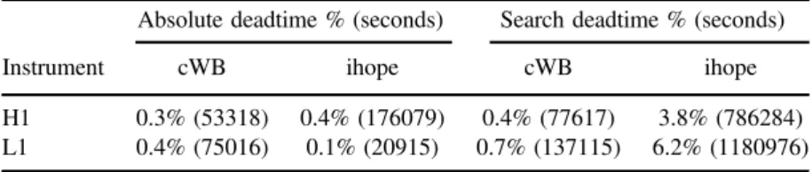
All LIGO-Virgo search groups used category 1 vetoes to omit unusable segments of data; as a result their primary effect was in the reduction in analysable time over which searches were performed. This impact is magnified by search requirements on the duration for analysed segments, with the cWB and ihope searches requiring a minimum of 316 and 2064 s of contiguous data respectively. Table 2 outlines the absolute deadtime (fraction of science-quality data removed) and the search deadtime (fractional reduction in analysable time after category 1 vetoes and segment selection). At both sites the amount of science-quality time flagged as category 1 is less than half of one percent, highlighting the stability of the instrument and its calibration. However, the deadtime introduced by segment selection is significantly higher, especially for the CBC analysis. The long segment duration requirement imposed by the ihope pipeline results in an order of magnitude increase in search deadtime relative to absolute deadtime.
5.1.2. Categories 2 and 3. The higher category flags were used to identify likely noise artefacts. Category 2 veto segments were generated from auxiliary data whose correlation with the GW readout has been firmly demonstrated by instrumental commissioning and investigations. Category 3 includes veto segments from less well understood statistical correlations between noisy data in an auxiliary channel and the GW readout. Both the ihope and cWB search pipelines produce afirst set of candidate event triggers after application of category 2 vetoes, and a reduced set after application of category 3.
The majority of category 2 veto segments were generated in low-latency by the DMT and include things like photodiode saturations, digital overflows, and high seismic and other environmental noise. At category 3, the HVeto [41], UPV [42], and bilinear-coupling veto [51] algorithms were used, by the burst and CBC analyses respectively, to identify coupling between auxiliary data and the GW readout.
Table3 gives the absolute, relative, and cumulative deadtimes of these categories after applying category 1 vetoes and segment selection criteria, outlining the amount of analysed time during which event triggers were removed. As with category 1, category 2 vetoes have deadtime (1)%, but with significantly higher application at L1 compared to H1. This is largely due to one flag used to veto the final 30 s before any lock loss, due to observed instrumental instability, combined with the relative abundance of short data-taking segments
Table 2.Summary of the reduction in all time and analysable time by category 1 veto segments during S6.
Absolute deadtime % (seconds) Search deadtime % (seconds)
Instrument cWB ihope cWB ihope
H1 0.3% (53318) 0.4% (176079) 0.4% (77617) 3.8% (786284)
for L1. Additionally, photodiode saturations and computational timing errors were more prevalent at the LLO site than at LHO and so contribute to higher relative deadtime.
Category 3flags contributed (10)% deadtime for each instrument. While this level of deadtime is relatively high, as we shall see, the efficiency of these flags in removing background noise events makes such cuts acceptable to the search groups.
Figure12shows the effect of category 3 vetoes on the background events from the cWB pipeline; these events were identified in the background from time time-slides and are plotted using the SNR reconstructed at each detector. This search applies category 2 vetoes in memory, and does not record any events before this step, so efficiency statements are only available for category 3. The results are shown after the application of a number of network-and signal-consistency checks internal to the pipeline that reject a large number of the loud events. As a result, the background is dominated by low SNR events, with a small number of loud outliers. At both sites, DQ vetoes applied to this search have cumulative EDR ⩾5 at SNR 3, with those at L1 removing the tail above SNR 20. However, despite the reduction, this search was still severely limited by the remaining tail in the multi-detector background distribution [7].
Figure13shows the effect of category 2 and 3 vetoes on the background from the CBC ihope pipeline; this search sees a background extending to higher SNR. As shown, the background is highly suppressed by DQ vetoes, with an efficiency of 50% above SNR 8, and 80% above∼100 at both sites. The re-weighted SNR statistic, as defined in [13], is highly effective in down-ranking the majority of outliers with high matched-filter SNR, but a non-Gaussian tail was still present at both sites. Category 3 vetoes successfully removed this tail,
Figure 12.The effect of category 3 vetoes on the cWB pipeline for (a) H1 and (b) L1. The left panels show the reduction in event rate, while the right panels show the cumulative veto efficiency, both as a function of single-detector SNR.
reducing the loudest event at H1 (L1) from a re-weighted SNR of 16.0 (15.3) to 11.1 (11.2). Search sensitive distance was roughly inversely proportional to the χ2-weighted SNR of the
loudest event, and so reducing the loudest event by ∼30% with ∼10% deadtime can be estimated as a factor of ∼2.5 increase in detectable event rate.
5.2. DQ in searches for long-duration signals
In searches for both continuous GWs and a SGWB, the duration and stationarity of data from each detector were the key factors in search sensitivity. These analyses integrate over the entire science run in order to maximize the SNR of a low-amplitude source. Accordingly, they
Table 3.Summary of the absolute, relative, and cumulative deadtimes introduced by category 2 and 3 veto segments during S6. The relative deadtime is the additional time removed by category 3 not vetoed by category 2, and cumulative deadtime gives the total time removed from the analysis.
H1 L1
Deadtime type Cat. cWB ihope cWB ihope
Absolute % (s) 2 0.26% 0.77% 1.59% 1.53%
3 7.90% 9.26% 8.54% 7.03%
Relative % (s) 3 7.73% 9.00% 7.06% 6.10%
Cumulative % (s) 3 7.97% 9.71% 8.54% 7.54%
Figure 13.The effect of category 2 and jointly of category 2 and 3 vetoes on the CBC ihope pipeline for (a) H1 and (b) L1. The left panels show the reduction in event rate as a function of SNR, the centre panels show the reduction in event rate as a function of the χ2-weighted SNR, and the right panels show the cumulative efficiency as a function of SNR.
![Figure 1. Optical layout of the LIGO interferometers during S6 [21]. The layout differs from that used in S5 with the addition of the output mode cleaner.](https://thumb-eu.123doks.com/thumbv2/123doknet/6149547.157321/11.892.220.697.119.433/figure-optical-layout-interferometers-layout-differs-addition-cleaner.webp)