Ship Complexity Assessment at Concept Design Stage

(will be inserted by the editor)

Ship Complexity Assessment at Concept Design Stage

Received: date / Accepted: date

Abstract A innovative complexity metric has been in-troduced in this paper and provides a solution to com-pare similar or different ship types and size together at the contract design stage. The goal is to provide the designer with such information throughout the design process so that an efficient design is obtained at the first design run. Application and validation on a real pas-senger ships have shown that a significant correlation between the error of an engineer’s judgement of com-plexity and the cost assessment error can be obtained. It follows that this tool could be used to improve the knowledge of ship’s complexity at the contract design stage or even to try to optimise their design if the com-plexity criteria are not fixed by the shipowners. Keywords Design complexity · Shipbuilding · Cost assessment · Optimisation

1 Introduction

1.1 How to define complexity

The description and understanding of the complexity in the design stage remains an open problem in the ship-building industry. In contrast with the relative

simplic-J-D. Caprace

ANAST – University of Li`ege, 1 Chemin des chevreuils, 4000

Li`ege, Belgium

Tel.: +32-4-3669621 Fax: +32-4-3669133

E-mail: jd.caprace@ulg.ac.be P. Rigo

ANAST – University of Li`ege, 1 Chemin des chevreuils, 4000

Li`ege, Belgium

Tel.: +32-4-3669366 Fax: +32-4-3669133 E-mail: ph.rigo@ulg.ac.be

ity involved by few degrees of freedom, the behaviour of ships cannot be simply understood from knowledge about the behaviour of their individual parts.

Despite many years of research in this field, it is very hard to find a formal definition of a ”complex system” in the literature. Complexity is a term normally used to describe a characteristic, which is hard to define and even harder to quantify precisely.

In general usage, complexity often tends to be used to characterize something with many parts in intricate ar-rangements [Sim62]. Actually, in science there are vari-ous approaches to characterizing complexity, as diverse as they are different. We can take into account : en-gineering, IT technology, management, economy, arith-metic, statistics, data mining, life simulation, psychol-ogy, philosophy, information, linguistics, etc. This is just a small sample of the enormous diversity of consid-erations given to the concept of complexity. Many def-initions tend to postulate or assume that complexity expresses a condition of numerous elements in a sys-tem and numerous forms of relationships among the elements. At the same time, what is complex and what is simple is relative and changes with time.

In a series of observations about complex systems and the architecture of complexity, [Sim96] highlights some common characteristics:

– Most complex systems contains a lot of redundancy – A complex system consists of many parts

– There are many relationships/interactions among the parts

– The complex systems can often be described with a hierarchy; redundant components can be grouped together and considered as integrated units

A hierarchy is a system that is composed of inter-related subsystems, each of the latter being, in turn, hierarchic in structure until we reach the lowest level of the elementary subsystem. In their dynamics, hi-erarchies have a property, near-decomposability, that greatly simplifies the description of a complex system, and makes it easier to understand how the information needed for the development or reproduction of the sys-tem can be stored in reasonable way.

In the everyday use of the word ”complexity”, a part A may be considered more complex than B, if A is more difficult to design and to manufacture than B. This subjective measure of complexity is however not sufficient for engineering analysis.

Complexity has captured the interest of engineers for many years, and a lot of various definitions are given in the literature [RTJS03]. Nowadays, more and more systems and technologies contain an overwhelm-ing complexity. This issue requires methods to break them down into a more understandable way, hence the need to define and measure complexity.

Industry has already attempted to measure com-plexity using empirical measures. The problem is that this results in a proliferation of possible measures: typ-ical examples include the number of items in the ship, analysis of production sequence and assemblies, etc. Having so many metrics offers problems. How do you know you are using the most appropriate ones or that you have sufficient accuracy? How can you tell if com-plexity is bring reduced if one measure falls but another rises?

Various researchers have recognised the importance of objectively measuring complexity, as an aid to ad-dressing the cause of such engineering and management related problems [Chr94] [LTCC97] [CES+_{00]. Our first}

objective is to decide what complexity is. Then a model of how to measure it can be produced.

1.2 Objectives of a ship design complexity metric As the complexity of a ship increases, the Life Cycle Costs (LCC) of the ship will typically increase as well. Also, a complex ship is commonly the result of a lengthy and complicated, and therefore, costly design process. Furthermore, because of the interconnection of various components and sub-assemblies in a complex ship, the engineering change process is often a complex and cum-bersome task. Next, manufacturing of a complex ship entails adaptation of complex process plans and sophis-ticated the manufacturing tools and technologies. Ad-ditionally, a complex ship results in a complex supply

chain which introduces various managerial and logistic problems. Finally, serviceability in a complex ship is a challenging issue due as well to the existence of numer-ous failure modes with multiple effects having varying levels of predictability.

Therefore, it is beneficial to objectively measure the complexity of ships in order to systematically reduce their inessential details. The main objective of this study is to define a quantitative measures of complexity that can be evaluated from a ship model at the early stage of the project design. This complexity measure of a de-sign should be able to guide the dede-signer in creating a product with the most cost effective balance of manu-facturing and assembly difficulty. The goal is to provide the designer with such information throughout the de-sign process so that an efficient dede-sign is produced in the first instance.

In terms of the manufacturing processes of ships, as-sembly costs and quality of the end product, complexity plays a vital role in the achievement of the best design. Unfortunately, little has been achieved in the area of complexity metrics that can be used in a useful way. One survey by [VV01] shows that from a series of stud-ies devoted to complexity, only 20% have attempted to produce some sort of quantification, thus considerable further research is required to make complexity a prac-tically useful concept.

One outlook of this work is the development of the means to quantify the complexity of a ship and the definition of measures to be used in conjunction with other metrics such as the assessment of production cost. Complexity is not defined in a quantifiable manner by the authors cited here, and thus considerable further re-search is required to make complexity a practical useful concept for shipbuilding industry.

2 Definition of a ship design complexity

With the current trend towards building the more so-phisticated types of vessel, a more accurate cost as-sessment in early design of the project, reflecting the complexity of the ship structure, is becoming a pre-requisite.

The measurement of complexity can eliminate sub-jective estimations and help to detect the most cost-effective production architecture and to control the de-sign process, and draw attention to critical changes. It is widely accepted that is much more cost-effective to produce an initial design that is simple, feasible and

easy to assemble, instead of rectifying the design prob-lems after the product has reached the shop floor.

Such kinds of model would not only help to con-trol the design process, as they would constantly draw attention to critical changes, but they would also help to compare different design alternatives. Such compar-isons will ultimately point out which solution requires less design effort and lower production costs.

Several factors that will influence ship macro complex-ity have been identified. Our research explores the com-plexity of different types and sizes of ships (Ctyp) as

well as the complexity of ships with the same size and same type but different arrangements and equipments (Carr). The complexity model is given in the equation

1, where CT represents the total complexity and w1,

..., wi represents numerical constants called weighting

factors.

CT =

w1Ctyp+ w2Carr

w1+ w2

(1)

2.1 Complexity of different types of ship (Ctyp)

The comparison of performance indicators, such as complexity, should take into account the size and type of the ships and the extent to which the production is serialized and/or standardized.

In order to compare the workload required to build ships of different sizes and types, the unit of measure-ments usually used is the Compensated Gross Tonnage (CGT). The objective of CGT is to adjust shipbuilding output measurements to consider work content, or dif-ferences in construction complexity for different types and sizes of ships. For example, the labour input per Gross Ton for passenger vessels is much higher than for tankers.

The CGT concept was originally proposed by ship-builder associations and later adopted by the Organ-isation for Economic Co-operation and Development (OECD). The objective was to provide a more accurate measure of shipyard activity or shipbuilding workload than could be achieved by gross tonnage (GT) or dead-weight ton (DWT) measurements. After the proposal of the first version in the 1980s, the CGT system under-went a number of revisions in order to improve accuracy and better reflect changes in both ship design and ship-yard working methods. The version presently used was introduced in January 2007 [CES07]. This new system1

1 _{developed by the Community of European Shipyards}

As-sociations (CESA), the Shipbuilders Association of Japan (SAJ) and the Korean Shipbuilders Association (KSA)

adopts a formula for calculating the CGT (see equation 2) where the coefficients a and b depends only on the type of ship. Using it for commercial ships over a wide range of size, types, and countries gives man-hour/CGT values ranging from 10 to 60.

CGT = a × GTb (2)

Finally, the complexity of different types of ship can be measured by dividing CGT by GT. A high ratio is an indicator for more sophisticated and special ships. The higher complexity ships are passenger ships, fishing ves-sels and LNG carriers while the lower complexity ships are combined carriers, oil tankers and bulk carriers.

The CGT system has significant limitations and seems to be insufficient to understand and control compet-itiveness [Ber03]. Nevertheless, it has been acknowl-edged worldwide as the best unit of measurement of the shipbuilding industry output so far. A number of stud-ies have been published with suggestions for improv-ing the system or extendimprov-ing its applicability, [Bru06, Lam03].

How to assess the complexity of two ships with the same dimensions and the same type? It is a question we try to answer in the next section. Obviously the complexity of both ships is different due to the diversity of internal arrangements and equipments.

2.2 Complexity of same type of ships (Carr)

The complexity of ships of the same type and same size is very difficult to quantify in the early stage of the project when very little information is available. This section proposes a method to quantify the relative complexity of a ship based on a Multi-Criteria Anal-ysis (MCA). The PROMETHEE (Preference Ranking Organization METHod for Enrichment Evaluation) has been chosen to define a complexity metric of ships [BM92, BM03,BM05].

2.2.1 Definition of alternatives

The outcome of any decision making models depends on the information at its disposal and the type of this infor-mation may vary according to the context in which the ship is operated. Therefore it is useful for decision mak-ing models to consider all the information as a whole. In Multiple Criteria Decision Making (MCDM) the deci-sion making procedure is normally carried out by choos-ing between different elements that the decision maker

has to examine and to assess, using a set of criteria. These elements are called alternatives. In this study, we analysed 10 different passenger ships of approxima-tively the same size. These ships are numbered from SHIP01 to SHIP10. In order to define an upper and a lower limit for the complexity evaluated in this study, two ideal cases have been added: the BEST ship, with the smallest complexity and the WORST ship with the higher complexity. All the criteria for these two ideal cases have been respectively minimized and maximized.

2.2.2 Definition of criterion

The criterion represents the tools which enable alter-natives to be compared from the point of view of com-plexity. It must be remembered that the selection of cri-teria is of prime importance in the resolution of a given problem, meaning that it is vital to identify a coher-ent family of criteria. The number of criteria is heavily dependent on the availability of both quantitative and qualitative information and data.

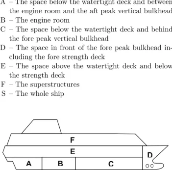
66 qualitative complexity criteria has been consid-ered in this study. These criteria were gathconsid-ered into 7 groups depending of the location of the criterion inside the ship (see Fig. 1). A college of experts defined these criteria based on their knowledge and expertise. Only the criteria available in the early stage of the project have been selected. The different groups are described below:

A – The space below the watertight deck and between the engine room and the aft peak vertical bulkhead B – The engine room

C – The space below the watertight deck and behind the fore peak vertical bulkhead

D – The space in front of the fore peak bulkhead in-cluding the fore strength deck

E – The space above the watertight deck and below the strength deck

F – The superstructures S – The whole ship

E D C B A F

Fig. 1 Ship complexity subdivision

The criterion for each groups are the following:

A – Propulsion Type, Rudder and Skeg, Stern Keel Shape, Stern Keel Width, Hawse Hole, Transversal Plating, Framing, Appendix, Tanks Position. B – Propulsion Type, Water Intake, Anti Roll Keel,

Engine Number, Oil Tank in DB, Stiffened Boxes. C – Tank Density, INOX Tank, Dynamic Stabilizer,

Chillers.

D – Bulb, Bow Truster, Bow Truster Device, Wash Board Shape, Chain Hole, Hawse Hole, Cranes. E – Transom Shape, Large Openings, Overhang, Tiers

Shape, Safety Davit.

F – Overhang Swim Pool, Fly Tower, Longitudinal Bulkhead, Balcony, SafetyBoat Bulkhead, Safety-Boat Height, Strength Hull, Aft Shape, Bulwark, Fore Slope, Fore Shape, Nbr Swim Pool, Openable Roof, Safety Davit, Theather.

S – Weight Stability Balance, Higher Deck Stress, Rule Class, ShipOwner Requirement, Pre Constract Study, Ice Class, Camber and Sheer, Fenders, Load Line Mark, Tumble Home, Gate Location, Gates Lines, Acoustic Level, Deck Levels, DB Height, DB Level, Lifts, Casing Long Position, Casing Trans Position, Atrium.

For each criterion the experts has defined different values ordered by ascendant complexity. For instance, the values for the propulsion type are: 2 pods, 3 to 4 pods, 2 to 4 shafting line and mixed. Each qualitative criterion correspond to a number which is considered to perform the MCDM.

2.2.3 Definition of weight and scenarios

The results of multi-criteria analysis hinge on the weight-ing allocated and thresholds set. The weights express the importance of each criterion and obviously may deeply influence the final outcome of the entire calcula-tion procedure. For some authors, the problem of how to determine the weights to be assigned is still unre-solved since the different outranking methods do not lay down any standard procedures or guidelines for de-termining them.

Group Weight distribution of scenarios

W1 W2 W3 W4 A 16.7% 14.3% 7.6% 5.8% B 16.7% 14.3% 10.2% 7.8% C 16.7% 14.3% 15.5% 11.9% D 16.7% 14.3% 6.9% 5.3% E 16.7% 14.3% 25.3% 19.5% F 16.7% 14.3% 34.5% 26.6% S 0% 14.3% 0.0% 23.0%

In this study, 4 scenarios with 4 different weight vectors were formulated to circumvent this problem (see Tab. 1):

1. The first scenario W1, representing a base-case, was

calculated by attributing equal weights to all group of criterion (16.7%) without considering the crite-rion applied to the group ”S”.

2. The second scenario W2 representing a base-case,

was calculated by attributing equal weights to all the groups of criterion (14.3%).

3. The third scenario W3was calculated based on the

majority opinion of the experts but without consid-ering the criterion in group ”S”.

4. The fourth scenario W4was calculated based on the

majority opinion of the experts. The weight to be adopted for the evaluation of complexity in scenario W4has been defined using F (26.6%), S (23%) and

E (19.5%). 2.2.4 Results

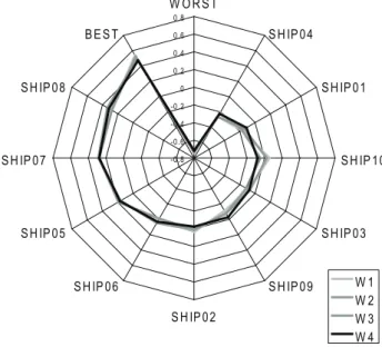
Fig. 2 presents the results of multi-criteria decision anal-ysis regarding preferences (global outranking flow φ) of the various ships expressed numerically. The higher the global outranking flow the better alternative. The small outranking flow for the SHIP04 indicates that is has a weak performance on most criteria, whereas the high outranking flow of SHIP08 is a sign that this alter-native is strong in most attribute values whatever the scenario. -0 .8 -0 .6 -0 .4 -0 .2 0 0 .2 0 .4 0 .6 0 .8 W O R S T S H IP 0 4 S H IP 0 1 S H IP 1 0 S H IP 0 3 S H IP 0 9 S H IP 0 2 S H IP 0 6 S H IP 0 5 S H IP 0 7 S H IP 0 8 B E S T W 1 W 2 W 3 W 4

Fig. 2 Aggregated outranking flows of the alternatives

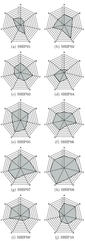
This result is confirmed by the spider diagram of the net flows of each criterion (see Fig. 3) which shows

that SHIP08 is the strongest alternative (maximization of the spider surface) and SHIP04 is the weakest al-ternative (minimization of the spider surface). Hence, also a change of the weight of the different criteria will show SHIP08 as the outstanding alternative (see Fig. 2). However, this assessment technique absolutely re-quires the existence of human expertise and know-how. Thus, we can not use it in all application cases.

Following the PROMETHEE method, the value of the global outranking flow φ can vary when we add new alternatives. Thus it is important to mention here that the value of the complexity is not an absolute value. The complexity must be used to compare the relative complexity of different ships together. Nevertheless we have demonstrated that the differences of the values of the global outranking flow φ of a same ship after adding a new ship in the analyses, vary as _(n−1)1 where n is the number of total alternatives (i.e. total number of ships). This means that out of 10 ships, the absolute value of the global outranking flow φ varies less than 1% when an alternative is added to the model.

Starting from the value of the global outranking flow φ of each alternative and the global outranking flow of the two ideal alternatives (i.e. the BEST ship and the WORST ship), the complexity metric Carr varying

between 0% and 100% has been defined following the equation 3. The result is presented in Fig. 4.

Carr = φ − φ BEST

φW ORST − φBEST

(3)

2.2.5 GAIA visualisation

We have also carried out a GAIA visualisation which provides a graphical representation of the various al-ternatives for different criteria and a π decision axis in which direction the best alternative is located according to the weight distribution. The GAIA plane is obtained by a projection of the information in the criteria space on a plane. The best plane is obtained by a Principal Components Analysis (PCA) technique. Through this projection some information is lost but most of the in-formation is preserved. In the present case the preserved information amounts to δ = 87.2%.

The GAIA plane given in Fig. 5 clearly confirms the previous results. Indeed, we can observe the following characteristics:

– The group of criterion B, F and D are more discrim-inating than E and C

– The group of criterion A, B, C express a similar preference

– The group of criterion F and D express a similar preference -0 .5 -0 .4 -0 .3 -0 .2 -0 .1 0 0 .1 0 .2 0 .3 0 .4 0 .5 A B C D E F S (a) SHIP01 -0 .5 -0 .4 -0 .3 -0 .2 -0 .1 0 0 .1 0 .2 0 .3 0 .4 0 .5 A B C D E F S (b) SHIP02 -0 .5 -0 .4 -0 .3 -0 .2 -0 .1 0 0 .1 0 .2 0 .3 0 .4 0 .5 A B C D E F S (c) SHIP03 -0 .5 -0 .4 -0 .3 -0 .2 -0 .1 0 0 .1 0 .2 0 .3 0 .4 0 .5 A B C D E F S (d) SHIP04 -0 .5 -0 .4 -0 .3 -0 .2 -0 .1 0 0 .1 0 .2 0 .3 0 .4 0 .5 A B C D E F S (e) SHIP05 -0 .5 -0 .4 -0 .3 -0 .2 -0 .1 0 0 .1 0 .2 0 .3 0 .4 0 .5 A B C D E F S (f) SHIP06 -0 .5 -0 .4 -0 .3 -0 .2 -0 .1 0 0 .1 0 .2 0 .3 0 .4 0 .5 A B C D E F S (g) SHIP07 -0 .5 -0 .4 -0 .3 -0 .2 -0 .1 0 0 .1 0 .2 0 .3 0 .4 0 .5 A B C D E F S (h) SHIP08 -0 .5 -0 .4 -0 .3 -0 .2 -0 .1 0 0 .1 0 .2 0 .3 0 .4 0 .5 A B C D E F S (i) SHIP09 -0 .5 -0 .4 -0 .3 -0 .2 -0 .1 0 0 .1 0 .2 0 .3 0 .4 0 .5 A B C D E F S (j) SHIP10

Fig. 3 Spider representation of ranking matrix for each

al-ternative

– The group of criterion A, B, C are independent re-garding group F and D

– SHIP08, SHIP07 and SHIP05 are the best alterna-tives considering the complexity

In order to study the behaviour of the decision model, we implemented different scenarios with different weights. For all weight distributions, the n decision vector re-mains oriented towards the same sector of the diagram. Such variation in weights can easily be handled and visualized on the GAIA plane. It can be noticed that the alternatives SHIP08 and SHIP07 are still the best choice whatever the scenario.

2.2.6 Sensitivity analysis

Sensitivity analysis has been carried out to study the subjective weights assigned to the criteria. The results has demonstrated the high weight stability of each sce-nario. The weight stability intervals give for each cri-terion family the limits within which its weight can be modified without changing the complete φ ranking. The stability intervals are valid only when a single weight is modified at a time and all the other weights vary proportionally to keep the sum of weight equal to 0.

2.2.7 Comparison with the expert intuition

A comparison between the intuitive ship complexity provided by the experts (Cexpert) and the complexity

(Carr) assessed in this study has been carried out. Fig

4 shows the results of this comparison. We can see that

0% 10% 20% 30% 40% 50% 60% 70% 80% 90% 100% W O R S T S H IP 0 4 S H IP 0 1 S H IP 1 0 S H IP 0 3 S H IP 0 9 S H IP 0 2 S H IP 0 6 S H IP 0 5 S H IP 0 7 S H IP 0 8 B E S T Carr Experts

Fig. 4 Comparison of the complexity with expert intuition

Fig. 5 GAIA view of criterion, alternatives and scenarios

the experts have a relative good intuition of the com-plexity of the ships except for SHIP05. Nevertheless, the ordering provided by the expert is quite similar to the ordering provided by the presented method. How-ever, some differences appear regarding the quantitative value of ship complexity.

-50% -40% -30% -20% -10% 0% 10% 20%

SHIP01 SHIP10 SHIP03 SHIP09 SHIP05 SHIP07 SHIP08

DeltaComplexity DeltaCost

Fig. 6 Comparison between delta complexity and delta cost

One of the viewpoints of the study was that the mis-judgement of experts concerning the complexity of the vessels (Carr− Cexpert) may explain the error of

eval-uating the cost of the ship at the pre contract design stage (Costeval− Costmeas); i.e. the difference between

the cost evaluated (Costeval) and the cost measured

after the end of the project (Costmeas). The result of

this comparison is shown in Fig. 6. Note that the cost error has only been provided for 7 ships. We can ob-serve a small correlation (R2_{= 0.601) between the}

mis-judgement of experts concerning the complexity of the vessels and the error of the cost evaluation at the pre contract design stage. Obviously the complexity of the ships cannot explain all the differences. When estimat-ing the cost or the complexity of a ship; there is always uncertainty as to the precise content of all the items in the estimate, how the work will be performed, what work conditions will be like when the project is exe-cuted and so on. These uncertainties are risks for the project. Some refer to these risks as ”known-unknowns” because the estimator is aware of them and, based on past experience, can even estimate their probable value. We have shown in this study that the misjudgement of the complexity of ships by the experts can explain a part of the cost evaluation error.

3 Conclusions

Complexity can be seen as a critical problem in de-sign that is needed to be reduced as much as possible. For example, complexity is associated with the diffi-culty of solving design problems, the combinatorial size

of the search space, and the variety of the generated de-signs. Notably, the complexity of solving design prob-lems occurs not only because these probprob-lems are of-ten intractable, ill-defined or ill-understood, but also because they involve many different participants, with many different goals and needs.

In order to solve these problem, different kinds of ship design complexity were investigated. A global complex-ity has been introduced in this paper and provides a solution to compare similar or different ship types and size together at the contract design stage. The results have shown that a significant correlation between the error of an engineer’s judgement of complexity and the cost assessment error can be obtained. It follows that this tool could be used to improve the knowledge of ship’s complexity at the contract design stage or even to try to optimise their design if the complexity criteria are not fixed by the shipowners.

The complexity measurement is an imperative basis for systematic optimality search, which is the essential process in design. The definition and the control of the upper limit of this metric will provide a good manage-ment tool to improve the overall design performance of ships.

We are well aware of the risk of creating a model that is mathematically viable but may not reflect reality be-cause of the quantity of assumptions made during the design process. The idea, nevertheless, is to define a model to make the complexity more approachable and, perhaps, even practical. Nobody has ever succeeded in giving a definition of the complexity which is mean-ingful enough to enable one to measure exactly how complex a system is. Ships cannot and should not be reduced to one single complexity measure. A ship is not only the end result but is also an entire system of manu-facturing, transport and economic evolution. Complex-ity should be seen as a decision tool aid.

Acknowledgements The authors thank University of Liege

and experts of some European shipyards for the collaboration in this project as well as the Belgian National Funds of Sci-entific Research (NFSR) for the financial support.

References

[Ber03] V. Bertram. Strategic Control of Productivity and

other Competitiveness Parameters. Proceedings of the I MECH E Part M, 217:61–70(10), 1 December 2003.

[BM92] J.P. Brans and B. Mareschal. Promethee v: Mcdm

problems with segmentation constraints. INFOR, 2(30), 1992.

[BM03] Jean-Pierre Brans and Bertrand Mareschal. How to Decide with PROMETHEE. 2003.

[BM05] Jean-Pierre Brans and Bertrand Mareschal.

Mul-tiple Criteria Decision Analysis: State of the Art Surveys, volume 78, chapter Promethee Methods, pages 163–186. Springer new york edition, 2005.

[Bru06] G. J. A. Bruce. A Review of the Use of

Com-pensated Gross Tonnage for Shipbuilding Perfor-mance Measurment. Journal of Ship Production, 22(2):99–104, 2006.

[CES+_{00] A. Calinescu, J. Efstathiou, S. Sivadasan,}

J. Schirn, and H. L. Huaccho. Complexity in Man-ufacturing: An Information Theoretic Approach. Conference on Complexity and Complex Systems in Industry, pages 19–20, 2000. University of War-wick, UK.

[CES07] KSA CESA, SAJ. Compensated Gross Ton (CGT)

System. Technical report, Organisation for Eco-nomic Co-operation and Development (OECD), 2007.

[Chr94] G. Chryssolouris. Measuring complexity in

manu-facturing systems. Technical report, University of Patras 26110 Greece, 1994. Working paper Depart-ment of Mechanical Engineering and Aeronautics.

[Lam03] Thomas Lamb. Methodology Used to

Calcu-late Naval Compensated Gross Tonnage Factors. Journal of Ship Production, 19(1):29–30, February 2003.

[LTCC97] G. Little, D. Tuttle, D. E. R. Clark, and J. A. Corney. Feature Complexity Index. Proceedings of Institution of Mechanical Engineers, 212:405– 412, 1997. Proceedings of Institution of Mechanical Engineers.

[RTJS03] C. RodriguezToro, S. Tate, G. Jared, and K. Swift. Complexity metrics for design. IMechE’03, 217, 2003.

[Sim62] Herbert A. Simon. The Architecture of

Complex-ity. In Proceeding of the American

Philosophi-cal Society, volume 106, pages 467–482, December 1962.

[Sim96] H.A. Simon. The Sciences of the Artificial. Mass.:

MIT Press, Cambridge, 1996.

[VV01] V.Tang and V.Salminen. Towards a Theory of

Complicatedness: Framework for Complex Systems Analysis and Design. 13th International Confer-ence on Engineering Design, page 8, Augustus 2001.