DOI:10.1051/0004-6361/201629869 c ESO 2017
Astronomy
&
Astrophysics
Complete spectral energy distribution of the hot,
helium-rich white dwarf RX J0503.9
−
2854
?
,
??
,
???
,
????
D. Hoyer
1, T. Rauch
1, K. Werner
1, J. W. Kruk
2, and P. Quinet
3, 41 Institute for Astronomy and Astrophysics, Kepler Center for Astro and Particle Physics, Eberhard Karls University, Sand 1,
72076 Tübingen, Germany
e-mail: rauch@astro.uni-tuebingen.de
2 NASA Goddard Space Flight Center, Greenbelt, MD 20771, USA
3 Physique Atomique et Astrophysique, Université de Mons – UMONS, 7000 Mons, Belgium
4 IPNAS, Université de Liège, Sart Tilman, 4000 Liège, Belgium
Received 10 October 2016/ Accepted 17 October 2016
ABSTRACT
Context. In the line-of-sight toward the DO-type white dwarf RX J0503.9−2854, the density of the interstellar medium (ISM) is very low, and thus the contamination of the stellar spectrum almost negligible. This allows us to identify many metal lines in a wide wavelength range from the extreme ultraviolet to the near infrared.
Aims.In previous spectral analyses, many metal lines in the ultraviolet spectrum of RX J0503.9−2854 have been identified. A com-plete line list of observed and identified lines is presented here.
Methods.We compared synthetic spectra that had been calculated from model atmospheres in non-local thermodynamical equilib-rium, with observations.
Results.In total, we identified 1272 lines (279 of them were newly assigned) in the wavelength range from the extreme ultraviolet to the near infrared. 287 lines remain unidentified. A close inspection of the EUV shows that still no good fit to the observed shape of the stellar continuum flux can be achieved although He, C, N, O, Al, Si, P, S, Ca, Sc, Ti, V, Cr, Mn, Fe, Cr, Ni Zn, Ga, Ge, As, Kr, Zr, Mo, Sn, Xe, and Ba are included in the stellar atmosphere models.
Conclusions.There are two possible reasons for the deviation between observed and synthetic flux in the EUV. Opacities from hitherto unconsidered elements in the model-atmosphere calculation may be missing, and/or the effective temperature is slightly lower than previously determined.
Key words. atomic data – line: identification – stars: abundances – stars: individual: RX J0503.9-2854 – virtual observatory tools
1. Introduction
The white dwarf (WD) RX J0503.9−2854 (henceforth RE 0503−289, WD 0501−289 McCook & Sion 1999a,b) was discovered in the ROSAT (ROentgen SATellite) wide field camera all-sky survey of extreme-ultraviolet (EUV) sources (Pounds et al. 1993). Barstow et al. (1993) reported its dis-covery by the Extreme Ultraviolet Explorer (EUVE), and identified it with a peculiar He-rich DO-type WD, namely MCT 0501−2858 in the Montreal-Cambridge-Tololo survey of southern hemisphere blue stars (Demers et al. 1986). They found that RE 0503−289 is located in a direction with very low density of the interstellar medium (ISM). In the line-of-sight
? Based on observations with the NASA/ESA Hubble Space
Tele-scope, obtained at the Space Telescope Science Institute, which is oper-ated by the Association of Universities for Research in Astronomy, Inc., under NASA contract NAS5-26666.
??
Based on observations made with the NASA-CNES-CSA Far Ul-traviolet Spectroscopic Explorer.
??? Based on observations made with ESO Telescopes at the La Silla
Paranal Observatory under program IDs 072.D-0362, 165.H-0588, and 167.D-0407.
???? Tables A.1–A.5 are only available at the CDS via anonymous ftp
tocdsarc.u-strasbg.fr (130.79.128.5) or via
http://cdsarc.u-strasbg.fr/viz-bin/qcat?J/A+A/598/A135
(LOS) toward RE 0503−289, Vennes et al. (1994) measured a column density of log(NHi/ cm−2) = 17.75−18.00 using EUVE photometry data.Rauch et al. (2016a) resolved at least two ISM components in the LOS toward RE 0503−289 based on high-resolution and high signal-to-noise ultraviolet (UV) spectroscopy performed by Far Ultraviolet Spectroscopic Explorer (FUSE) and Hubble Space Telescope/Space Telescope Imaging Spectrograph (HST/STIS) and measured a very low (EB−V= 0.015 ± 0.002) interstellar reddening.
The almost negligible contamination by ISM line absorp-tion allows us to identify even weak lines of many species from so far He up to trans-iron elements as heavy as Ba (Table 2). For reliable abundance analyses of these elements, a precise Teff and log g determination is a prerequisite to keep
error propagation as small as possible. An initial constraint of Teff= 60 000−70 000 K was given byVennes et al.(1994) from
EUV photometry. The first spectral analysis by means of non-local thermodynamic equilibrium (NLTE) stellar atmosphere models considering opacities of H, He, and C was published by Barstow et al. (1994). They found Teff= 60 000−80 000 K and
log(g/cm/s2) = 7.5−8.0.Dreizler & Werner(1996) used
ultra-violet (UV) spectra in addition and NLTE model atmospheres and determined Teff= 70 000 ± 5000 K and log g = 7.5 ± 0.5.
Table 1. History of Teffand log g determinations (cf.,Müller-Ringat 2013).
Teff/kK log g Model atmosphere Method Comment Reference
60−90 EUV, PM very low NHi Barstow et al.(1993)
60−80 EUV, OPT very low NHi Barstow et al.(1993)
60−80 7.5−8.0 He, HHeC NLTE, OPT, UV, EUV EUV problema Barstow et al.(1994)
60−70 EUV, PM very low NHi Vennes et al.(1994)
70b 7.0 HeCNOSiFeNi LTE, EUV, UV Polomski et al.(1995)
65c 7.5d HHeC NLTE, OPT no H detectable, upper
limit 5% (mass frac-tion)
Werner(1996)
70 7.5 HHeCNOSi NLTE, OPT, UV M= 0.49 M Dreizler & Werner(1996)
66.6−70.4 7.13−7.27 HHe LTE, UV M= 0.40 M Vennes et al.(1998)
70e 7.5e NLTE, diffusion no good fit achieved Dreizler(1999)
69−75 7.26−7.63 HHeC NLTE, OPT, UV, EUV EUV problema Barstow et al.(2000)
HHeCNOSiFeNi
65−70 7.5e HeCNi, HeONi NLTE, EUV EUV problema Werner et al.(2001)
70e 7.5e HHeCNOSiFeNi+ NLTE, UV EUV problema Barstow et al.(2007)
PS LTE
68−72 7.4−7.6 HeCNOAlSiPS+ NLTE, OPT, UV M= 0.514+0.15−0.05M Rauch et al.(2016a)
CaScTiVCrMnFeCrNi+ ZnGaGeAsKrZrMoSnXeBa
Notes. PM denotes photometry.(a)Section7,(b)adopted upper limit ofVennes et al.(1994),(c)adopted value close to lower limit ofBarstow et al.
(1994),(d)adopted fromBarstow et al.(1994),(e)adopted fromDreizler & Werner(1996).
(FUSE and HST/STIS) spectra and significantly reduced the er-ror limits to ±2000 K and ±0.1, respectively. Table1summarizes previous analyses.
2. Observations
In this paper, we used the observed spectra that are briefly de-scribed in the following. If they are compared to synthetic spec-tra, the latter are convolved with Gaussians to model the respec-tive instrument’s resolution.
Extreme ultraviolet: observations by the EUVE observatory were performed using the short-wavelength (70 Å < λ < 190 Å), the medium-wavelength (140 Å < λ < 380 Å), and the long-wavelength (280 Å < λ < 760 Å) spectrometers with a resolv-ing power of R ≈ 300. Details of the data reduction are given by Dupuis et al.(1995).
Far ultraviolet: spectra (910 Å < λ < 1190 Å, R ≈ 20 000) were obtained with FUSE. Their data IDs are M1123601 (2000-12-04), M1124201 (2001-02-02), and P2041601 (2000-12-05). The spectra were shifted to rest wavelengths and co-added. For details seeWerner et al.(2012b).
Ultraviolet: spectroscopy was performed with HST/STIS on 2014-08-14. Two observations with grating E140M (1144 Å < λ < 1709 Å, R ≈ 45 800) and two observations with grating E230M (1690 Å < λ < 2366 Å, 2277 Å < λ < 3073 Å, R ≈ 30 000) were co-added. These observations are retriev-able from the Barbara A. Mikulski Archive for Space Telescopes (MAST).
Optical: spectra (3290 Å < λ < 4524 Å, 4604 Å < λ < 5609 Å, 5673 Å < λ < 6641 Å) were obtained on 2000-09-09 and 2001-04-08 in the framework of the Supernova Ia Progenitor Survey project (SPY,Napiwotzki et al. 2001,2003). The Ultraviolet and Visual Echelle Spectrograph (UVES) attached to the Very Large Telescope (VLT) located at the European Southern Observatory (ESO) on Cerro Paranal in Chile was employed to achieve a res-olution of about 0.2 Å. In addition, we use a spectrum taken with
the Echelle Multi Mode Instrument (EMMI) attached to the New Technology Telescope (NTT; 1992-01, 4094 Å < λ < 4994 Å, resolution of about 3.0 Å).
Near infrared: spectroscopy (9500 Å < λ < 13 420 Å, R ≈950) was performed on 2003-12-10 using the Son-of-Isaac (SofI) instrument at the NTT. The spectrum used here was digi-tized with Dexter1from Fig. 1 inDobbie et al.(2005).
3. Model atmospheres and atomic data
The stellar model atmospheres used for this paper were calculated with our Tübingen NLTE Model Atmosphere Package (TMAP2, Werner et al. 2003, 2012a). They assume plane-parallel geometry, are chemically homogeneous, and in hydrostatic and radiative equilibrium. An adaptation is the New Generation Radiative Transport (NGRT) code (Dreizler & Wolff 1999;Schuh et al. 2002) that can consider diffusion in addition to calculate stratified stellar atmospheres.
The Tübingen Model Atom Database (TMAD3) provides
ready-to-use model atoms in TMAP format for many species up to Ba. TMAD has been constructed as part of the Tübingen contribution to the German Astrophysical Virtual Observatory (GAVO4).
Werner et al. (2012b) discovered lines of trans-iron ele-ments, namely Ga (atomic number Z = 31), Ge (32), As (33), Se (34), Kr (36), Mo (42), Sn (50), Te (52), I (53), and Xe (54), in the FUSE spectrum of RE 0503−289. For precise abun-dance determinations of these species, reliable atomic data is mandatory. For example, reliable transition probabilities are re-quired, not only for lines that are identified in the observation but for the complete model atoms that are considered in the model-atmosphere calculations. Due to the lack of such data, Werner et al. (2012b) were restricted to abundance determina-tions of Kr and Xe only.
1 http://dc.zah.uni-heidelberg.de/sdexter 2 http://astro.uni-tuebingen.de/~TMAP 3 http://astro.uni-tuebingen.de/~TMAD 4 http://www.g-vo.org
Table 2. Photospheric abundances (mass fraction) of RE 0503−289.
Element Abundance 1st Line identifications He 9.73 × 10⁻¹ Barstow et al.(1994) C 2.22 × 10⁻² Barstow et al.(1994) N 5.49 × 10⁻⁵ Dreizler & Werner(1996)
O 2.94 × 10⁻³ Polomski et al.(1995), Dreizler & Werner(1996) Al 5.01 × 10⁻⁵ Rauch et al.(2016a) Si 1.60 × 10⁻⁴ Polomski et al.(1995),
Dreizler & Werner(1996)
P 1.06 × 10⁻⁶ Vennes et al.(1998),Barstow et al. (2007)
S 3.96 × 10⁻⁵ Barstow et al.(2007) Ni 7.25 × 10⁻⁵ Barstow et al.(2000)
Zn 1.13 × 10⁻⁴ Rauch et al.(2014a) Ga 3.44 × 10⁻⁵ Werner et al.(2012b), Rauch et al.(2015b) Ge 1.58 × 10⁻⁴ Werner et al.(2012b), Rauch et al.(2012) As 1.60 × 10⁻⁵ Werner et al.(2012b) Se Werner et al.(2012b) Kr 5.04 × 10⁻⁴ Werner et al.(2012b), Rauch et al.(2016a) Zr 3.00 × 10⁻⁴ Rauch et al.(2016a) Mo 1.88 × 10⁻⁴ Rauch et al.(2016b) Sn 2.06 × 10⁻⁴ Werner et al.(2012b)
Te Werner et al.(2012b)
I Werner et al.(2012b)
Xe 1.26 × 10⁻⁴ Werner et al.(2012b),
Rauch et al.(2015a), Rauch et al.(2016a) Ba 3.57 × 10⁻⁴ Rauch et al.(2014b)
Notes. The reference for the 1st line identifications is given in the final column.
We initiated the calculation of new transition probabilities that were then used to determine the abundance of the respec-tive element. Table3gives an overview of the so far calculated data. To provide easy access to this data, the registered Tübingen Oscillator Strengths Service (TOSS) has been created within the GAVO project.
To construct model atoms for the use within TMAP, the el-ements given in Table3require the calculation of so-called su-per levels and susu-per lines with our Iron Opacity and Interface (IrOnIc,Rauch & Deetjen 2003) due to the very high number of atomic levels and lines. We transferred the TOSS data into Ku-rucz’s data format5that can be read by IrOnIc.
4. Radial velocity and gravitational redshift
To shift the observation to rest wavelength, we determined the radial velocity vradof RE 0503−289 from FUSE and HST/STIS
spectra. To measure the wavelengths of the line centers, we used IRAF6 to fit Gaussians to the line profiles. In total, we evalu-ated 100 lines in the FUSE wavelength range and 103 lines in
5 http://kurucz.harvard.edu/atoms.html
6 IRAF is distributed by the National Optical Astronomy Observatory,
which is operated by the Associated Universities for Research in As-tronomy, Inc., under cooperative agreement with the National Science Foundation.
Table 3. Newly calculated transition probabilities.
Element Ions Reference
Zn
iv–v
Rauch et al.(2014a)Ga
iv–vi
Rauch et al.(2015b)Ge
v–vi
Rauch et al.(2012)Kr
iv–vii
Rauch et al.(2016a)Zr
iv–vii
Rauch et al.(2016a)Tc
ii– vi
Werner et al.(2015)Mo
iv–vii
Rauch et al.(2016b)Xe
iv–vii
Rauch et al.(2015a,2016a)Ba
v–vii
Rauch et al.(2014b)20 25 30 35 950 1000 1050 1100 1150 20 25 30 35 1200 1250 1300 1350 1600 2000 2975 λ / Ao vra d / k m /s
Fig. 1.Determination of vrad from individual lines in the FUSE (top
panel) and HST/STIS observations (bottom). The full horizontal lines
indicate the average vrad for FUSE and HST/STIS, respectively. The
dashed lines show the 1σ error.
the STIS wavelength range (Fig.1). The averages are vFUSE
rad =
25.7 ± 4.2 km s−1 and vSTIS
rad = 25.8 ± 3.7 km s
−1. We adopted
the mean value of vrad = 25.7+3.6−4.0km s−1. From this value, the
gravitational redshift z has to be subtracted. To calculate z and the respective radial velocity, we created the GAVO tool Tübin-gen Gravitational REDshift calculator (TGRED, Fig.C.2). For RE 0503−289, we derive vgredrad = 15.5+6.7−4.6km s−1. The true radial velocity is then vRE 0503−289rad = 10.2+8.2−8.6km s−1.
5. Line identification
To unambiguously identify lines in our observed spectra (Sect. 2), we used the best synthetic model of Rauch et al. (2016a) and calculated additional spectra with oscillator strengths set to zero for individual elements. This allows to find weak lines, even if they are blended by stronger lines. The de-tection limit is an equivalent width of Wλ = 2 mÅ. Table 4 shows the total numbers of lines identified in the four wavelength ranges and the numbers of lines that were suited to determine Wλ
and vrad. The current line lists are presented in Tables A.1–A.5,
a regularly updated version is available online7.
7 http://astro.uni-tuebingen.de/~hoyer/objects/ RE0503-289
Table 4. Statistics of the identified (in brackets: newly identified in this paper) and unidentified lines in the observed spectra.
Wavelength Numbers of lines
Wλ vrad
range total identified unidentified
EUV 74 74(35) 0 0 0
FUV 616 536(55) 76 148 100
NUV 790 579(120) 211 252 103
optical 83 83(69) 0 0 0
NIR 2 2(0) 0 0 0
Notes. The last two columns give the numbers of lines that were used
to measure their equivalent widths Wλand vrad(Fig.1), respectively.
6. Visualization and online line list
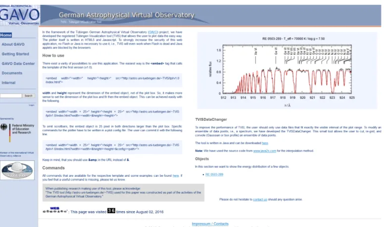
In the framework of the Tübingen GAVO project, we have devel-oped the registered Tübingen VISisualization tool (TVIS) that allows the user to plot any data in an easy way on the WWW. The plotter itself is written in HTML5 and Javascript. To strongly increase the security of this web application, no Flash or Java is necessary to use it, meaning that TVIS will even work when Flash is dead and Java applets are blocked by the browsers.
The comparison of our best model spectra with the available observation of RE 0503−289 in the EUV, FUV, NUV, and optical wavelength ranges was realized with TVIS and is shown online8.
FiguresB.1toB.3show the FUV to optical range.
7. Is there still an EUV problem in RE 0503–289?
To analyze the EUVE observation, Barstow et al. (1995) used NLTE model atmospheres that were calculated with the code that is nowadays called TMAP. A synthetic spectrum (scaled to match the observed EUV flux) that was calculated from a model with Teff= 70 000 K, log g = 7.0, C/He = 1%, and N/He =
0.01% (the latter being number ratios) reproduced well the ob-servation. A major problem arose, however, from the fact that the model flux (reddened and interstellar neutral hydrogen ab-sorption considered) in the wavelength range 228 Å < λ < 400 Å was about an order of magnitude higher than observed. Only models with Teff < 65 000 K produced an acceptable
fit. He
i
λ 5875.62 Å (2p3Po–3d3D) in the optical wavelengthrange (e.g., in spectra taken with the TWIN spectrograph at the Calar Alto observatory and in SPY spectra,Dreizler & Werner 1996; Rauch et al. 2016a) establishes a stringent constraint of Teff= 70 000 ± 2000 K.
Werner et al. (2001) calculated TMAP models that were composed of He, C, O, and the iron-group elements (Ca–Ni). Interstellar He
i
absorption was applied in addition to that of Hi
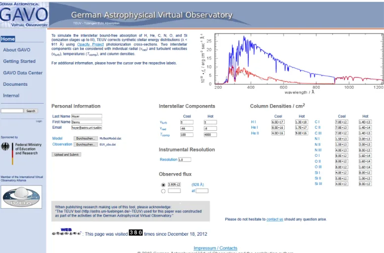
. The flux discrepancy was reduced (model flux three times higher than observed) but the basic problem, finding an agreement at Teff= 70 000 K, was not solved.Müller-Ringat(2013) created the Tübingen EUV absorption tool (TEUV, Fig.C.1), that corrects synthetic stellar fluxes for ISM absorption for λ < 911 Å. Presently, only radiative bound-free absorption of the lowest ionization states of H, He, C, N, and O is simulated. Opacity Project data (Seaton et al. 1994) is used for the photoionization cross-sections. These consider, for ex-ample, autoionization features. For this paper, Si has been added to TEUV. Two interstellar components with different radial and turbulent velocities, temperatures, and column densities can
8 http://astro.uni-tuebingen.de/~TVIS/objects/ RE0503-289 lo g ( fλ / e rg /c m 2 /s /A o ) H Iis C IV H e II 2 -3 H e II 3 -7 H e II 3 -6 H e II 4 -5 H e II 5 -7 -15 -14 -13 -12 -11 5000 10000 H e II O IV H e II C IV C II I O II I C IV O V C IV O II I C II I O II I C II I O IV C II I O II I O IV C IV -13 -12 -11 -10 300 400 500 600 λ / Ao
Fig. 2.Determination of EB−V. Top: reddening with EB−V= 0.00026
applied to our synthetic spectrum in the wavelength range from the EUV
to the NIR. Bottom: same like top panel, for EB−V= 0.00016 (blue),
0.00026 (red), and 0.00036 (green) in the EUV wavelength range. Prominent lines are marked.
be considered.Müller-Ringat (2013) calculated TMAP models (Teff= 70 000 K, log g = 7.5) that included He, C, N, O, and the
iron-group elements. Although Kurucz’s line lists were strongly extended in 2009 (Kurucz 2009, 2011), and about a factor of ten more iron-group lines were considered, the EUV model flux was about twice as high as that observed. To match the observed EUV flux, Teffhad to be reduced to <∼65 000 K.
Rauch et al.(2016a) determined Teff= 70 000 ± 2000 K and
log g= 7.5 ± 0.1 in a detailed reanalysis of optical and UV spec-tra. They included 27 elements, namely He, C, N, O, Al, Si, P, S, Ca, Sc, Ti, V, Cr, Mn, Fe, Cr, Ni, Zn, Ga, Ge, As, Kr, Zr, Mo, Sn, Xe, and Ba, in their models. From these, we calculated the EUV spectrum (228 Å ≤ λ ≤ 910 Å) with 1601 atomic levels treated in NLTE, considering 2481 lines of the elements He–S and about 30 million lines of the elements with Z ≥ 20. The frequency grid comprised 174 873 points with∆λ ≤ 0.005 Å.
Figure 2 demonstrates the determination of the interstel-lar reddening. We apply the reddening data of Morrison & McCammon (1983, provided for 1.26 Å ≤ λ ≤ 413 Å and extrap-olated toward the He
i
ground-state threshold) and Fitzpatrick (1999, λ ≥ 911 Å). Between the Hei
ground-state edge and the Hi
Lyman edge, only absorption due to Hi
is consid-ered. To determine EB−V, we normalized our models to the2MASS H brightness (14.766 ± 0.063, Cutri et al. 2003a,b). To match the observed flux level between about 400 Å to 600 Å, EB−V= 0.00026 ± 0.00003 is necessary. This is less than
Teff / K = 70000 66000 lo g ( fλ / e rg /c m 2 /s /A o ) H e II C IV H e II C IV O II I O IV O II I S c V II N IV O II I C IV O IV O II I C IV O IV H e II C IV C II I S c V II C II I S c V II N IV O II I N II I N IV C II I O II I C IV O V C II I O V C IV O II I X e V I K r V I K r V II C II I K r V I C II I C II I X e V I C IV H e I C IV H e I X e V I O II I C IV H e I C IV O V O IV C IV O II I -12 -11 Teff / K = 70000 Ni x 200 He+C+N+O+Fe+Ni -12 -11 240 260 280 300 320 340 360 380 400 420 440 460 480 500 520 540 560 580 600 620 λ / Ao
Fig. 3.Comparison of the EUVE observation (gray line in both panels) with our models. Top panel: two models with Teff= 70 000 K (red) and
Teff= 66 000 K (blue). Identified photospheric lines are marked at the top. Bottom panel: three models with Teff= 70 000 K. Red, thick line: model
from the top panel, red, dashed line: model with 200 times increased Ni abundance, blue, thin line: model that considered only opacities of He, C, N, O, Fe, and Ni.
reproduce the observed FUSE flux level. With the Galactic red-dening law ofGroenewegen & Lamers(1989, log(NHi/EB−V =
21.58 ± 0.1) and the total cloud column density of interstellar H
i
of 1.5 ± 0.2 × 1018 cm−2 (measured from L β,Rauch et al.2016a), we can calculate EB−V= 0.00039+0.00017−0.00012which is within
error limits well in agreement with our result.
A close look at the EUV wavelength range shows still a sig-nificant difference between model and observation (Fig.3, top panel), most prominent between 250 Å and 400 Å and between 504 Å and 550 Å. Our present models reduced the deviation by about a factor of two compared the models of Werner et al. (2001). The EUV problem cannot be solved by using a cooler model, even at Teff= 66 000 K, which is already outside the error
range of Teff= 70 000 ± 2000 K given byRauch et al. (2016a),
no sufficient improvement is achieved. The impact of metal opacities is demonstrated in Fig.3 by a model that considered only opacities from He, C, N, O, Fe, and Ni with same abun-dance ratios like our best model. To test the impact of addi-tional opacity, we artificially increased the Ni abundance by fac-tor of 200 to match the model’s flux to the observed between 250 Å and 280 Å. This reduced the flux discrepancy between
300 Å and 400 Å as well while the wavelength region above the He
i
ground-state threshold is unaffected. However, we conclude that even in our advanced models opacity is missing from ele-ments that are hitherto not considered. To include, for example, other trans-iron elements requires detailed laboratory measure-ments of their spectra and the extensive calculation of transition probabilities.8. What is the nature of RE 0503–289?
RE 0503−289 was first classified to be a DO-type WD (Barstow et al.1993). Its optical spectrum exhibits an absorption trough around CIVλλ 4646.62−4687.95 Å and HeIIλ 4685.80 Å. This
trough is the spectroscopic criterion for the H-deficient PG 1159-type stars (e.g., Werner & Herwig 2006). Figure 4 shows the comparison of the wavelength region around this trough for the PG 1159 prototype PG 1159−035 (V? GW Vir, WD 1159−035, Teff= 140 000 ± 5000 K, log g = 7.0 ± 0.5, Jahn et al. 2007)
and the O(He)-type WD KPD 0005+5106 (WD 0005+511, Teff= 195 000 ± 15 000 K, log g = 6.7 ± 0.2, Werner & Rauch
PG 1159-035 Teff= 140 000 K log g = 7.0 RE 0503-289 Teff= 70 000 K log g = 7.5 PG 0122+200 Teff= 80 000 K log g = 7.5 N V 3 s -3 p O IV 5 g -6 h C IV 5 d -6 f C IV 5 f-6 g C IV 5 g -6 h C IV 5 g -6 f C IV 5 f-6 d C IV 6 d -8 f C IV 6 f-8 g C IV 6 g -8 h C IV 6 h -8 i C IV 6 h -8 g C IV 6 g -8 f H e II 3 -4 C IV 6 f-8 d 0.5 1.0 1.5 2.0 4620 4640 4660 4680 4700 4720 λ / Ao r e la ti v e f lu x
Fig. 4. Section of the optical spectra of PG 1159−035 (from SPY,
shifted by 0.3 in flux units), RE 0503−289 (EMMI), and PG 0122+200
(Keck, shifted by −0.3; from top to bottom) around the PG 1159
absorp-tion trough. For RE 0503−289, the synthetic spectrum ofRauch et al.
(2016a) is overplotted (red line). The green, dashed lines indicate the continuum level.
than RE 0503−289. The strengths of the PG 1159 absorption troughs are almost the same for the much hotter PG 1159−035 and RE 0503−289, although their photospheric C abundances are significantly different, ≈48% by mass (Jahn et al. 2007) and ≈2%, respectively. The cool PG 1159-type star PG 0122+200 has about 22% of C in its photosphere (Werner & Rauch 2014).
In a log Teff–log g diagram (Fig.5), RE 0503−289 is located
at the so-called PG 1159 wind limit (Unglaub & Bues 2000, their Fig. 13, digitized with Dexter) that was predicted for a ten-times-reduced mass-loss rate (line A, calculated with ˙M = 1.29 × 10⁻¹⁵L1.86 from Bloecker 1995; Pauldrach et al. 1988).
This line approximately separates the regions that are populated by PG 1159-type stars and DO-type WDs. Lines B and C in Fig.5show where the photospheric C content is reduced by fac-tors of 0.5 and 0.1, respectively, when using the mass-loss rate given above. To the right of line D, no PG 1159 star is located.
Werner et al. (2014) suggested a mass ratio C/He = 0.02 to conserve previously assigned spectroscopic classes. How-ever, PG 1159 stars span a wide range of C/He (0.03−0.33, Werner et al. 2014).
RE 0503−289 is located close to line B ofUnglaub & Bues (2000) in Fig.5, that is, its C abundance should be already re-duced by a factor of 0.5. Thus, it is likely that RE 0503−289 had a C/He ≈ 0.05 in its antecedent PG 1159-star phase. Even now, its C/He lies a bit higher than 0.02 and RE 0503−289 may be classified as a PG 1159 star as well. This is corroborated by the still high efficiency of radiative levitation that is responsible for the extremely high overabundances of trans-iron elements (Rauch et al. 2016b). However, the transition from a PG 1159-type star to a DO-1159-type star is smooth and RE 0503−289 is an ideal object to study this in detail. Unfortunately, the strong ra-diative levitation of trans-iron elements wipes out all informa-tion about their asymptotic giant branch (AGB) abundances and RE 0503−289 is not suited to constrain AGB nucleosynthesis models. A B C D O(He) PG 1159 DO 0 .5 1 4 0 .5 3 0 0 .5 4 2 0.5 6 5 0.5 84 0.6 09 0.6 64 0.7 41 0.8 69 RE 0503-289 8.5 8.0 7.5 7.0 6.5 5.4 5.2 5.0 4.8 log (Teff/ K) lo g ( g / c m /s 2 )
Fig. 5.Location of RE 0503−289 and related objects (Hügelmeyer et al. 2006; Kepler et al. 2016; Reindl et al. 2014b,a; Werner & Herwig
2006) in the log Teff–log g plane (cf., http://www.star.le.ac.
uk/~nr152/He.htmlfor stellar parameters). Evolutionary tracks for
H-deficient WDs (Althaus et al. 2009) labeled with their respective
masses in M are plotted for comparison. Transition limits predicted
byUnglaub & Bues(2000) are indicated (see text for details).
9. Results
RE 0503−289 fulfills criteria of PG 1159 star and of DO-type WD classifications. The presence of the strong PG 1159 ab-sorption trough around HeIIλ 4685.80 Å (Fig. 4) shows that
RE 0503−289 could be classified as a PG 1159 star, although its C abundance would then be the lowest of this group. It is located close to the so-called PG 1159 wind limit (Fig.5), meaning that it is close to the regime in which gravitation will dominate and pull metals down, out of the atmosphere. The strongly increased abundances of trans-iron elements, however, indicate that radia-tive levitation is still efficiently counteracting this process. Thus, RE 0503−289 has not arrived in its final stage of evolution. For-mally, due to its log g > 7, the DO-type WD classification is right.
In the observed spectra, we identified 1272 lines in the wave-length range from the extreme ultraviolet to the near infrared. 287 lines remain unidentified. The best model of Rauch et al. (2016a) reproduces well most of the identified lines.
The EUV problem (Sect. 7) – the difference between ob-served and synthetic flux in the EUV is still present. Our ad-vanced model atmospheres include opacities of 27 metals but their flux in the EUV is still partly about a factor of approxi-mately two too high compared with the observation. We expect that missing metal opacities are the reason for this discrepancy. Acknowledgements. D.H. and T.R. are supported by the German Aerospace Center (DLR, grants 50 OR 1501 and 05 OR 1507, respectively). The Ger-man Astrophysical Virtual Observatory (GAVO) project at Tübingen had been supported by the Federal Ministry of Education and Research (BMBF, 05 AC 6 VTB, 05 AC 11 VTB). Financial support from the Belgian FRS-FNRS is also acknowledged. P.Q. is research director of this organization. Some of the data presented in this paper were obtained from the Mikulski Archive for Space Telescopes (MAST). STScI is operated by the Association of Universities for Research in Astronomy, Inc., under NASA contract NAS5-26555. Support for MAST for non-HST data is provided by the NASA Of-fice of Space Science via grant NNX09AF08G and by other grants and contracts. We thank Ralf Napiwotzki for putting the reduced ESO/VLT spectra at our disposal. The TEUV tool (http://astro-uni-tuebingen.
de/~TEUV), the TGRED tool (http://astro-uni-tuebingen.de/~TGRED),
the TIRO service (http://astro-uni-tuebingen.de/~TIRO), the TMAD service (http://astro-uni-tuebingen.de/~TMAD), the TOSS service
(http://astro-uni-tuebingen.de/~TOSS), and the TVIS tool (http://
part of the activities of the German Astrophysical Virtual Observatory. This work used the profile-fitting procedure OWENS developed by M. Lemoine and the FUSE French Team. This research has made use of NASA’s Astrophysics Data System and of the SIMBAD database operated at CDS, Strasbourg, France.
References
Althaus, L. G., Panei, J. A., Miller Bertolami, M. M., et al. 2009,ApJ, 704, 1605
Barstow, M. A., Wesemael, F., Holberg, J. B., et al. 1993,Adv. Space Res., 13, 281
Barstow, M. A., Holberg, J. B., Werner, K., Buckley, D. A. H., & Stobie, R. S. 1994,MNRAS, 267, 653
Barstow, M. A., Holberg, J. B., Koester, D., Nousek, J. A., & Werner, K. 1995, in White Dwarfs (Berlin: Springer Verlag), eds. D. Koester, & K. Werner,Lect. Notes Phys., 443, 302
Barstow, M. A., Dreizler, S., Holberg, J. B., et al. 2000,MNRAS, 314, 109
Barstow, M. A., Dobbie, P. D., Forbes, A. E., & Boyce, D. D. 2007, in 15th European Workshop on White Dwarfs, eds. R. Napiwotzki, & M. R. Burleigh,
ASP Conf. Ser., 372, 243
Bloecker, T. 1995,A&A, 299, 755
Cutri, R. M., Skrutskie, M. F., van Dyk, S., et al. 2003a, 2MASS All Sky Catalog of point sources
Cutri, R. M., Skrutskie, M. F., van Dyk, S., et al. 2003b,VizieR Online Data
Catalog: II/246
Demers, S., Beland, S., Kibblewhite, E. J., Irwin, M. J., & Nithakorn, D. S. 1986,
AJ, 92, 878
Dobbie, P. D., Burleigh, M. R., Levan, A. J., et al. 2005,A&A, 439, 1159
Dreizler, S. 1999,A&A, 352, 632
Dreizler, S., & Werner, K. 1996,A&A, 314, 217
Dreizler, S., & Wolff, B. 1999,A&A, 348, 189
Dupuis, J., Vennes, S., Bowyer, S., Pradhan, A. K., & Thejll, P. 1995,ApJ, 455, 574
Fitzpatrick, E. L. 1999,PASP, 111, 63
Groenewegen, M. A. T., & Lamers, H. J. G. L. M. 1989,A&AS, 79, 359
Hügelmeyer, S. D., Dreizler, S., Homeier, D., et al. 2006,A&A, 454, 617
Jahn, D., Rauch, T., Reiff, E., et al. 2007,A&A, 462, 281
Kepler, S. O., Pelisoli, I., Koester, D., et al. 2016,MNRAS, 455, 3413
Kurucz, R. L. 2009, in AIP Conf. Ser. 1171, eds. I. Hubeny, J. M. Stone, K. MacGregor, & K. Werner, 43
Kurucz, R. L. 2011,Can. J. Phys., 89, 417
McCook, G. P., & Sion, E. M. 1999a,ApJS, 121, 1
McCook, G. P., & Sion, E. M. 1999b,VizieR Online Data Catalog: III/210 Morrison, R., & McCammon, D. 1983,ApJ, 270, 119
Müller-Ringat, E. 2013, Dissertation, University of Tübingen, Germany,http: //nbn-resolving.de/urn:nbn:de:bsz:21-opus-67747
Napiwotzki, R., Christlieb, N., Drechsel, H., et al. 2001,Astron. Nachr., 322, 411
Napiwotzki, R., Christlieb, N., Drechsel, H., et al. 2003,The Messenger, 112, 25
Pauldrach, A., Puls, J., Kudritzki, R. P., Mendez, R. H., & Heap, S. R. 1988,
A&A, 207, 123
Polomski, E. F., Vennes, S., & Chayer, P. 1995, in BAAS, AAS Meeting Abstracts, 27, 1311
Pounds, K. A., Allan, D. J., Barber, C., et al. 1993,MNRAS, 260, 77
Rauch, T., & Deetjen, J. L. 2003, in Stellar Atmosphere Modeling, eds. I. Hubeny, D. Mihalas, & K. Werner,ASP Conf. Ser., 288, 103
Rauch, T., Werner, K., Biémont, É., Quinet, P., & Kruk, J. W. 2012,A&A, 546, A55
Rauch, T., Werner, K., Quinet, P., & Kruk, J. W. 2014a,A&A, 564, A41
Rauch, T., Werner, K., Quinet, P., & Kruk, J. W. 2014b,A&A, 566, A10
Rauch, T., Hoyer, D., Quinet, P., Gallardo, M., & Raineri, M. 2015a,A&A, 577, A88
Rauch, T., Werner, K., Quinet, P., & Kruk, J. W. 2015b,A&A, 577, A6
Rauch, T., Gamrath, S., Quinet, P., et al. 2016a,A&A, 590, A128
Rauch, T., Quinet, P., Hoyer, D., et al. 2016b,A&A, 587, A39
Reindl, N., Rauch, T., Werner, K., et al. 2014a,A&A, 572, A117
Reindl, N., Rauch, T., Werner, K., Kruk, J. W., & Todt, H. 2014b,A&A, 566, A116
Schuh, S. L., Dreizler, S., & Wolff, B. 2002,A&A, 382, 164
Seaton, M. J., Yan, Y., Mihalas, D., & Pradhan, A. K. 1994,MNRAS, 266, 805
Unglaub, K., & Bues, I. 2000,A&A, 359, 1042
Vennes, S., Dupuis, J., Bowyer, S., et al. 1994,ApJ, 421, L35
Vennes, S., Dupuis, J., Chayer, P., et al. 1998,ApJ, 500, L41
Werner, K. 1996,A&A, 309, 861
Werner, K., & Herwig, F. 2006,PASP, 118, 183
Werner, K., & Rauch, T. 2014,A&A, 569, A99
Werner, K., & Rauch, T. 2015,A&A, 583, A131
Werner, K., Deetjen, J. L., Rauch, T., & Wolff, B. 2001, in 12th European Workshop on White Dwarfs, eds. J. L. Provencal, H. L. Shipman, J. MacDonald, & S. Goodchild,ASP Conf. Ser., 226, 55
Werner, K., Deetjen, J. L., Dreizler, S., et al. 2003, in Stellar Atmosphere Modeling, eds. I. Hubeny, D. Mihalas, & K. Werner,ASP Conf. Ser., 288, 31
Werner, K., Dreizler, S., & Rauch, T. 2012a, TMAP: Tübingen NLTE Model-Atmosphere Package, Astrophysics Source Code Library
[record ascl:1212.015]
Werner, K., Rauch, T., Ringat, E., & Kruk, J. W. 2012b,ApJ, 753, L7
Werner, K., Rauch, T., & Kepler, S. O. 2014,A&A, 564, A53
Appendix A: Identified and unidentified lines in the spectrum of RE 0503–289
Tables A.1−A.5 are available at the CDS.
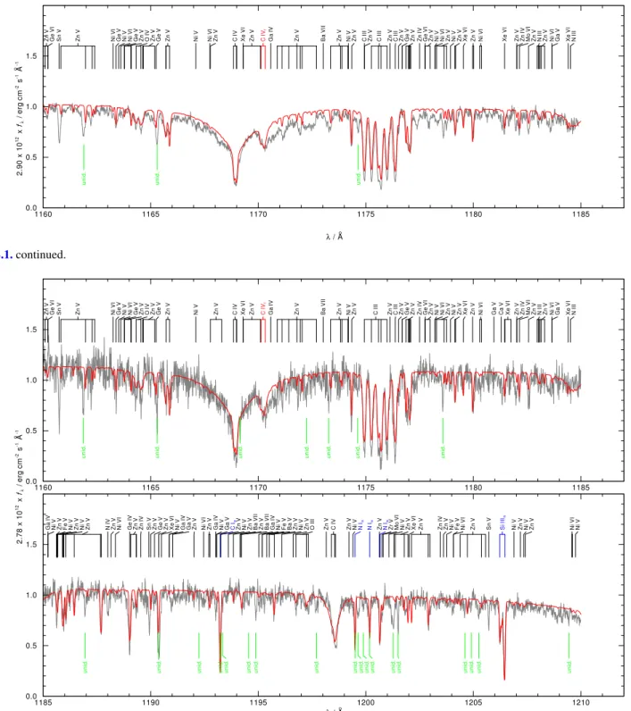
Appendix B: Observed spectra of RE 0503–289 compared with our best model
In the following figures, we show the comparison of our syn-thetic spectra with the FUSE (Fig. B.1, HST/STIS (Fig. B.2, and optical (Fig. B.3 observations. A visualization via TVIS is available at http://astro.uni-tuebingen.de/~TVIS/ objects/RE0503-289 H I 0 1 -2 5is H I 0 1 -2 4is H I 0 1 -2 3is H I 0 1 -2 2is H I 0 1 -2 1is H I 0 1 -2 0is H I 0 1 -1 9is H I 0 1 -1 8is H I 0 1 -1 7is H I 0 1 -1 6is X e V I N IIis H I 0 1 -1 5is H I 0 1 -1 4is H I 0 1 -1 3is G e V I H I 0 1 -1 2is G e V I K r V II H I 0 1 -1 1is X e V I G e V I K r V I G e V I H I 0 1 -1 0is O IV O IV N IV H I 0 1 -0 9is N IV O IV N IV B a V S V N IV G e V I B a V II G e V I H I 0 1 -0 8is G e V I K r V I G e V I X e V I G e V I O Iis G e V I G e V G e V I Z n V G e V I Z n V H I 0 1 -0 7is K r V I O V Z n V S V I Z n V G e V I u n id . 0.0 0.5 1.0 1.5 910 915 920 925 930 935 X e V I N i V G e V I O Iis G e IV B a V I H e II B a V II H I 0 1 -0 6is G e IV G e V I O IV G e V I B a V II H e II G e V B a V II G a V N i V I K r V I S V I X e V I B a V Z n V G e V I C IV N IV G e V I O Iis B a V H e II H I 0 1 -0 5is O V B a V II P IV O Iis N Iis G e V I G a IV G e V I B a V I N Iis N Iis G a V I Z n V N Iis G e V I G a V N IV G e V I K r V I G a IV G e V I S V G e V I G e V H e II u n id . u n id . u n id . 0.0 0.5 1.0 1.5 935 940 945 950 955 960 λ / Ao 3 .5 7 x 1 0 1 2 x fλ / e rg c m -2 s -1 A o-1
G e V I X e V I G a V P Iis N Iis G e V I N Iis K r V I N i V G e V B a V II G e V I X e V I G e V I F e V G e V I B a V II K r V I X e V I G e V G e V I O Iis O Iis O Iis H e II D Iis H I 0 1 -0 4is O IV G e V I O Iis C II Iis C II I G e V B a V II G e V I F e V G a V I F e V G a V N II I X e V I N II I G a V I K r V I G e V I G a V X e V I C II I G a V I G e V I Z n V F e V G a V I M o V F e V G a V G e V u n id . u n id . u n id . u n id . 0.0 0.5 1.0 1.5 960 965 970 975 980 985 M o V O IV G e V A s V F e Iis G e V O Iis O IV O Iis F e V O IV O Iis S i IIis O V N II I G e V N II I G e V H e II G e V I B a V II O IV O IV X e V II M o V I X e V II X e V I S e IV P V F e V B a V II Z n V S V I C a II I Z r V C II I Z r V G a V K r V I F e V G a V I G e V G a V I G e V C II I G e V I G e V N i V I G a V I Z n V F e V G a V I G e V B a V II B a V O II I G e V I N i V G a V I N i V I Z n V F e V N i V I G a V u n id . u n id . u n id . u n id . u n id . 0.0 0.5 1.0 1.5 985 990 995 1000 1005 1010 λ / Ao 3 .4 3 x 1 0 1 2 x fλ / e rg c m -2 s -1 A o-1 Fig. B.1.continued. G a V I B a V II N i V F e V G a V I K r V I F e V N i V G e V I M o V F e V Z n V G a V G e V I G a V Z n V G a V K r V I C II I G e V X e V I Z n V G a V Z n V G e V H e II D Iis H I 0 1 -0 3is A s V Z n V P IV N i V I O V Iis O V I G a V Z n V G e V N i V I C a II I G a V u n id . u n id . u n id . u n id . u n id . u n id . u n id . u n id . u n id . u n id . u n id . u n id . u n id . u n id . 0.0 0.5 1.0 1.5 1010 1015 1020 1025 1030 1035 G e V Z n V N i V Z n V N IV Z n V N IV C IIis Z n V C IIis N i V I N i V Z n V O V Iis O V I Z n V G e V M o V I Z n V G a V O Iis G e V G e V I S V Z n V F e V O II I Z n V G e V I N i V B a V II B a V Z n V B a V Z n V S n IV Z n IV K r V I O IV G e V G a V Z n V O IV Z n V M o V I G a V O IV B a V G e V A r Iis G e V Z n V G e V G a V O IV A s V B a V Z n V K r V I Z n V M o V K r V I G e V I Z n V Z r V I X e V I N i V B a V II Z n V G e V B a V O IV G e V O V Z n V B a V II S e V I Z n V G a V Z n V G e V Z n V u n id . u n id . u n id . u n id . u n id . u n id . u n id . u n id . u n id . u n id . u n id . 0.0 0.5 1.0 1.5 1035 1040 1045 1050 1055 1060 λ / Ao 3 .9 8 x 1 0 1 2 x fλ / e rg c m -2 s -1 A o -1 Fig. B.1.continued.
Z n V C IV K r V I G e V Z n V O IV Z n V N i V O IV G a V O IV Z n V G e V G a V Z n V G e V I S e V I G e V Z r V I Z n V G e V Z n V C IV S i IV Z n V B a V O IV Z n V G e V Z r V G a V G e V G a V Z n V C II I G e V Z n V G e V Z n V G a V T e V I Z n V G e V Z n V G e V G a V Z n V G e V Z n V N i V I O IV Z n V N i V I Z n V X e V II G a V G e V O IV G a V N i V I G a V X e V I Z n V G e V Z n V O IV N i V G a V F e V O IV N IIis H e II u n id . u n id . u n id . u n id . u n id . u n id . u n id . u n id . 0.0 0.5 1.0 1.5 1060 1065 1070 1075 1080 1085 O IV Z n V G e V G a V G e V G a V N i V I Z n V S n V G e V N i V I Z n V N i V I X e V I Z n V G a V G e V Z n V N IV O IV G e V G e V I Z n V G a V N i V I S e V G a V Z n V N i V I G e V Z n V O IV G e V B a V G e V Z n V O IV G e V O IV Z r V I F e V G a V G e V M o V G a V M o V Z n V X e V I B a V Z n V G e V G a V Z n V N IV G a V F e V N i V I N i V G a V B a V G e V C IVf Z n V X e V I B a V I C IV O IV G e V Z n V G e V Z n V G a V O IV u n id . u n id . u n id . u n id . u n id . u n id . u n id . u n id . u n id . 0.0 0.5 1.0 1.5 1085 1090 1095 1100 1105 1110 λ / Ao 3 .8 8 x 1 0 1 2 x fλ / e rg c m -2 s -1 A o-1 Fig. B.1.continued. X e V I Z n V N i V I Z n V N i V I N i V B a V II Z n V B a V Z n V B a V Z n V G e V Z n V G a V Z n V B a V Z n V G e V Z n V S V I P V P Vis G a V Z r V I Z n V Z r V N i V B a V II Z n V I V I Z n V F e V I N i V I Z n V O V Z n V G e V S V B a V S i IV Z n V G e V Z n V G a V G e V N i V I N i V F e V Z n V G e V C II I M o V C II I M o V G a V Z n V G a V P V P Vis G a V Z n V S i IV B a V G a V S V Z n V N i V I Z n V F e V I G e V G a V Z n V G e V N i V I Z n V N i V I Z n V G a V Z n V G a V Z n V B a V Z n V S n V Z n V S V N Iis N Iis N Iis u n id . u n id . u n id . u n id . u n id . u n id . u n id . u n id . u n id . u n id . 0.0 0.5 1.0 1.5 1110 1115 1120 1125 1130 1135 Z n V G a V Z n V N i IV X e V I Z n V N i V I Z n V M o V Z n V G e V Z n V N i V I C II I Z n V B a V II Z n V N i V I Z n V F e IIis B a V II F e II I Z n V N i V I Z n V N i V I X e V I N i V F e Iis Z n V G e V N i V I Z n V G a V M o V Z n V N i V I G a V Z n V O II I S e V N i V Z n V G a IV Z n V Z r V I Z n V N i V B a V Z n V N i V Z n V B a V II B a V O II I Z n V N i V I G a V Z n V B a V Z n V F e V I G a V F e V I N i V F e V I Z n V G a V Z n V F e V N i V I Z n V N i V I Z n V B a V II B a V Z n V N i V N i V I Z n V u n id . u n id . u n id . u n id . u n id . u n id . u n id . u n id . 0.0 0.5 1.0 1.5 1135 1140 1145 1150 1155 1160 λ / Ao 2 .5 8 x 1 0 1 2 x fλ / e rg c m -2 s -1 A o-1 Fig. B.1.continued.
Z n V G e V I S n V Z n V N i V I G e V N i V N i V I G e V Z n V O IV Z n V G e V Z n V N i V N i V I Z n V C IV X e V I Z n V C IVf G a IV Z n V B a V II Z n V N i V Z n V C II I Z n V C II I Z n V C II I Z n V G e V Z n V Z n IV G e V I Z n V N i V N i V I Z n V N i V Z n V X e V I Z n V N i V I X e V I Z n V Z n IV M o V I Z n V N II I Z n V N i V I G a V X e V I N II I u n id . u n id . u n id . 0.0 0.5 1.0 1.5 1160 1165 1170 1175 1180 1185 λ / Ao 2 .9 0 x 1 0 1 2 x f λ / e rg c m -2 s -1 A o-1 Fig. B.1.continued. Z n V G e V I S n V Z n V N i V I G e V N i V N i V I G e V Z n V O IV Z n V G e V Z n V N i V Z n V C IV X e V I Z n V C IV f G a IV Z n V B a V II Z n V N i V Z n V C II I Z n V C II I Z n V G e V Z n V Z n IV G e V I Z n V N i V N i V I Z n V N i V Z n V X e V I Z n V N i V I G a V C a V X e V I Z n V Z n IV M o V I Z n V N II I Z n V N i V I G a V X e V I N II I u n id . u n id . u n id . u n id . u n id . u n id . u n id . 0.0 0.5 1.0 1.5 1160 1165 1170 1175 1180 1185 G a IV N i V Z n V F e V N i V Z n V N i V Z n V N IV Z n V N i V I G e IV Z n V Z n IV S n V Z n V G e V Z n V X e V I N i V G a IV G a V Z n V N i V I Z n V G a IV N i V G a V C Iis Z n V N i V Z n V B a V II Z n V B a V II G a IV N i V F e V B a V Z n V N i V Z n V O II I Z n V C IV Z n V N i V N Iis N Iis Z n V N Iis Z r V M o V I N i V Z n V X e V I Z n V Z n IV Z n V N i V F e V N i V I Z n V S n V S i II Iis N i V Z n V N i V Z n V N i V I N i V u n id . u n id . u n id . u n id . u n id . u n id . u n id . u n id . u n id . u n id . u n id . u n id . u n id . u n id . u n id . u n id . u n id . u n id . 0.0 0.5 1.0 1.5 1185 1190 1195 1200 1205 1210 λ / Ao 2 .7 8 x 1 0 1 2 x fλ / e rg c m -2 s -1 A o-1
C II I N i V S i IV X e V I H e II C IV X e V I N i V G e V Z n IV Z n V Z n IV N i V Z n V N IV S b V Z n V N i V S e V G a IV N i V I X e V I Z n IV N i V M o V G e IV C IV N i V Z n V N i V N i V X e V I N i V N i V I N i V Z n IV u n id . u n id . u n id . u n id . u n id . u n id . u n id . u n id . u n id . u n id . u n id . u n id . u n id . u n id . 0.0 0.5 1.0 1.5 1210 1215 1220 1225 1230 1235 Z n V B a V N i V F e V G a IV Z n V N i V N i V I N i V F e V G a IV N i V Z n V N i V N V Z n V N i V G a V I N i V N i V I K r V N i V N i V I N i V N i V I N i V O IV N V O IV Z n IV N i V N i V I O V Z n V N i V N i V I N i V N i IV N i V G a IV Z r V N i V Z n V N i V Z n V C II I X e V I N i V B a V B a V II Z n V N i V Z n V N i V Z n V N i V Z n V N i V N i IV N i V N i V I F e IV N i V N i V I N i V B a V N i V K r V N i V F e V N i V B a V II Z n V N i V F e V I N i V O IV C II I N i V Z n V N i V N i V I Z n V O IV Z n V G a IV N i V u n id . u n id . u n id . u n id . u n id . u n id . u n id . u n id . u n id . u n id . u n id . u n id . 0.0 0.5 1.0 1.5 1235 1240 1245 1250 1255 1260 λ / Ao 2 .3 0 x 1 0 1 2 x fλ / e rg c m -2 s -1 A o-1 Fig. B.2.continued. Z n V S i IIis N i V Z r V Z n V N i V N i V I N i V N IV N i V N i V I N i V F e V Z n V N i V M o V I Z n V N i V G a IV N i V N i V I N i V Z n V N i V I Z r V G a V C a V I Z n IV F e V N i V G a IV F e V N i V Z n IV N i V Z n V S V N i V I N i V Z n V N i V N II I N IV N II I M o V I N i V N IV G e V I N i V X e V I N i V N IV Z n IV N i V N IV N i V Z n V N i V F e V Z n V Z n IV N i V Z n IV N i V Z n V N i V Z n V G a IV N i V X e V I Z n IV N i V I Z n V N i V Z n IV N i V Z n V N i V Z n IV X e V I S n V N i V B a V Z n IV Z n V Z n IV N i V Z n IV u n id . u n id . u n id . u n id . u n id . u n id . u n id . u n id . u n id . u n id . u n id . u n id . u n id . u n id . u n id . u n id . u n id . u n id . u n id . u n id . u n id . u n id . u n id . u n id . u n id . 0.0 0.5 1.0 1.5 1260 1265 1270 1275 1280 1285 N i V G e V I G a IV N i V Z n V N i V Z n IV N i V Z n IV N i V Z n V Z n IV Z n V S n V N i V Z n V O IV Z n V F e V N i V C II I N IV F e V I Z n IV O IV N i V X e V I G a IV Z n V N i V Z n IV C a V N i V O Iis N i V Z n V N i V G a IV Z r V N i V F e V N i V Z n V N i V F e V Z n IV N i V Z n IV Z r V N i V Z n V C II I Z n V N IV N i V u n id . u n id . u n id . u n id . u n id . u n id . u n id . u n id . u n id . u n id . u n id . u n id . u n id . 0.0 0.5 1.0 1.5 1285 1290 1295 1300 1305 1310 λ / Ao 2 .1 4 x 1 0 1 2 x fλ / e rg c m -2 s -1 A o-1 Fig. B.2.continued.
N i V G a V N i V Z n V Z n IV B a V N i II I N i V S n IV N i V G a IV N i V N i V I N i V C IV N i V C IV Z n V B a V Z n V N II I N i V Z n IV Z n V N i V F e V K r V N i V Z n IV N i V Z n IV N i V Z r V N i V F e V I N i V Z n V N IV Z n V Z n IV N IV O IV N i V Z n IV N i V Z n V Z n IV F e IV N i V N i V I N i V Z r V N i V Z n IV N i V C IIis N i V u n id . u n id . u n id . u n id . u n id . u n id . u n id . 0.0 0.5 1.0 1.5 1310 1315 1320 1325 1330 1335 N i V Z n IV N i V G a IV O IV Z n V Z n IV N i V X e V I N i V G a IV B a V Z n V N i V Z n IV O IV Z n IV N i V Z n IV Z n V O II I Z n V N i V C II I Z n IV B a V Z n IV N i V C IV Z r V N i V Z n IV Z r V Z n IV u n id . u n id . u n id . u n id . u n id . u n id . 0.0 0.5 1.0 1.5 1335 1340 1345 1350 1355 1360 λ / Ao 1 .9 8 x 1 0 1 2 x fλ / e rg c m -2 s -1 A o-1 Fig. B.2.continued. Z n IV B a V II Z n IV B a V II Z n IV O V S r V N i V M o V Z n IV M o V Z n IV N i V Z r V Z n IV C II I K r V N i V u n id . u n id . u n id . u n id . u n id . u n id . u n id . u n id . u n id . 0.0 0.5 1.0 1.5 1360 1365 1370 1375 1380 1385 P V N i V Z n IV F e V Z n IV K r V Z n IV N i V Z n IV F e V N i V Z n V K r V Z n IV K r V S i IV B a V II Z n IV F e V I N i V N i IV B a V II N i V Z n V K r V S i IV B a V II K r V K r V I N i V u n id . u n id . u n id . u n id . u n id . u n id . u n id . 0.0 0.5 1.0 1.5 1385 1390 1395 1400 1405 1410 λ / Ao 1 .5 8 x 1 0 1 2 x fλ / e rg c m -2 s -1 A o-1 Fig. B.2.continued.
Z n IV N i V B a V S r V K r V Z n IV Z n V B a V II Z n IV C II I M o V I C II I B a V II K r V u n id . u n id . u n id . u n id . u n id . u n id . u n id . 0.0 0.5 1.0 1.5 1410 1415 1420 1425 1430 1435 K r V S n IV K r V X e V I C IV S V N IV B a V II N i V F e V B a V Z n V N i V Z n V G e V Z n V Z n IV u n id . u n id . u n id . 0.0 0.5 1.0 1.5 1435 1440 1445 1450 1455 1460 λ / Ao 1 .4 0 x 1 0 1 2 x fλ / e rg c m -2 s -1 A o-1 Fig. B.2.continued. Z n V Z n IV Z n V B a V II Z n V B a V II Z n V N i V I B a V II Z n V B a V N i V Z n V F e V Z n V B a V II C II I B a V II G e V C II I Z n V C II I N i V C II I M o V I B a V II B a V Z n IV F e V B a V II N i V Z n V N i V I Z n V N V N i V I G e V G e IV C II I O II I F e V G e V Z n V G e IV S V X e V I Z n V G e V u n id . u n id . u n id . u n id . u n id . u n id . u n id . 0.0 0.5 1.0 1.5 1460 1465 1470 1475 1480 1485 1490 1495 1500 1505 1510 Z r V I Z n V K r V N i V Z r V I B a V II N i V S i IIis Z n V C II I N i V I Z n V C II I C IV Z n IV Z n V O IV N i V G e V Z n IV u n id . u n id . u n id . 0.0 0.5 1.0 1.5 1510 1515 1520 1525 1530 1535 1540 1545 1550 1555 1560 λ / Ao 1 .1 7 x 1 0 1 2 x fλ / e rg c m -2 s -1 A o-1 Fig. B.2.continued.
G e V Z n V G e V K r V Z n V G e V M o V C II I N II I C II I Z n V G e V C II I Z n IV C II I G e V B a V II K r V G e V B a V II C IV M o V K r V M o V C II I Z r V I K r V G e V B a V M o V I B a V II O V G e V Z r IV O IV Z n V G e V u n id . u n id . u n id . u n id . u n id . 0.0 0.5 1.0 1.5 1560 1565 1570 1575 1580 1585 1590 1595 1600 1605 1610 G e V X e V I N V Z n V C II I G e V Z n V B a V II Z r V C IV H e II C II I M o V C IV B a V II Z n V G e V u n id . u n id . u n id . u n id . 0.0 0.5 1.0 1.5 1610 1615 1620 1625 1630 1635 1640 1645 1650 1655 1660 λ / Ao 1 .0 8 x 1 0 1 2 x fλ / e rg c m -2 s -1 A o-1 Fig. B.2.continued. O IV M o V X e V I B a V II M o V Z n V G e V Z r V I Z n V M o V I O V N IV M o V u n id . u n id . u n id . 0.0 0.5 1.0 1.5 1660 1665 1670 1675 1680 1685 1690 1695 1700 1705 1710 B a V II M o V M o V I N IV M o V I M o V S i IV Z r V S i IV O IV S V B a V II O IV B a V II X e V I M o V Z r V I B a V II u n id . u n id . u n id . u n id . 0.0 0.5 1.0 1.5 1710 1715 1720 1725 1730 1735 1740 1745 1750 1755 1760 λ / Ao 8 .0 8 x 1 0 1 3 x fλ / e rg c m -2 s -1 A o-1 Fig. B.2.continued.
O II I K r V B a V II O II I M o V O II I M o V B a V II C II I X e V I B a V II M o V X e V I M o V N II I u n id . u n id . u n id . u n id . u n id . u n id . u n id . 0.0 0.5 1.0 1.5 1760 1765 1770 1775 1780 1785 1790 1795 1800 1805 1810 N IV B a V II K r V I M o V B a V II M o V u n id . u n id . u n id . u n id . u n id . 0.0 0.5 1.0 1.5 1810 1815 1820 1825 1830 1835 1840 1845 1850 1855 1860 λ / Ao 6 .4 0 x 1 0 1 3 x fλ / e rg c m -2 s -1 A o-1 Fig. B.2.continued. Z n IV G e V Z n IV X e V I B a V II C II I K r V I u n id . u n id . u n id . u n id . u n id . u n id . u n id . 0.0 0.5 1.0 1.5 1860 1865 1870 1875 1880 1885 1890 1895 1900 1905 1910 O II I K r V I O IV C II I O IV N i V I C II I B a V II K r V I u n id . u n id . 0.0 0.5 1.0 1.5 1910 1915 1920 1925 1930 1935 1940 1945 1950 1955 1960 λ / Ao 5 .7 3 x 1 0 1 3 x fλ / e rg c m -2 s -1 A o-1 Fig. B.2.continued.
X e V I M o V S V I G e V X e V I S V S V I M o V I B a V II M o V I C II I u n id . u n id . 0.0 0.5 1.0 1.5 1960 1965 1970 1975 1980 1985 1990 1995 2000 2005 2010 C II I N IV K r V I u n id . u n id . u n id . u n id . u n id . u n id . 0.0 0.5 1.0 1.5 2010 2015 2020 2025 2030 2035 2040 2045 2050 2055 2060 λ / Ao 4 .0 0 x 1 0 1 3 x fλ / e rg c m -2 s -1 A o-1 Fig. B.2.continued. S V N IV C II I C IV u n id . u n id . 0.0 0.5 1.0 1.5 2060 2065 2070 2075 2080 2085 2090 2095 2100 2105 2110 S i IV K r V K r V I O IV X e V I S V u n id . 0.0 0.5 1.0 1.5 2110 2115 2120 2125 2130 2135 2140 2145 2150 2155 2160 λ / Ao 3 .7 5 x 1 0 1 3 x fλ / e rg c m -2 s -1 A o-1 Fig. B.2.continued.
C II I K r V C II I H e II K r V M o V I 0.0 0.5 1.0 1.5 2160 2165 2170 2175 2180 2185 2190 2195 2200 2205 2210 H e II X e V I H e II K r V u n id . u n id . u n id . u n id . 0.0 0.5 1.0 1.5 2210 2215 2220 2225 2230 2235 2240 2245 2250 2255 2260 λ / Ao 2 .7 4 x 1 0 1 3 x fλ / e rg c m -2 s -1 A o-1 Fig. B.2.continued. M o V I C IV S i IV C II I H e II 0.0 0.5 1.0 1.5 2260 2265 2270 2275 2280 2285 2290 2295 2300 2305 2310 X e V I K r V C IV C IV u n id . u n id . 0.0 0.5 1.0 1.5 2310 2315 2320 2325 2330 2335 2340 2345 2350 2355 2360 λ / Ao 2 .4 2 x 1 0 1 3 x fλ / e rg c m -2 s -1 A o-1 Fig. B.2.continued.
O II I H e II C IV u n id . 0.0 0.5 1.0 1.5 2360 2365 2370 2375 2380 2385 2390 2395 2400 2405 2410 X e V I P V K r V G e IV O II I P V O IV O II I 0.0 0.5 1.0 1.5 2410 2415 2420 2425 2430 2435 2440 2445 2450 2455 2460 λ / Ao 2 .1 5 x 1 0 1 3 x fλ / e rg c m -2 s -1 A o-1 Fig. B.2.continued. B a V II N IV C II I G e IV O IV B a V II O IV u n id . 0.0 0.5 1.0 1.5 2460 2465 2470 2475 2480 2485 2490 2495 2500 2505 2510 H e II O IV C IV O IV O II I u n id . u n id . 0.0 0.5 1.0 1.5 2510 2515 2520 2525 2530 2535 2540 2545 2550 2555 2560 λ / Ao 2 .0 1 x 1 0 1 3 x fλ / e rg c m -2 s -1 A o-1 Fig. B.2.continued.
S V I C IV O II I X e V O II I u n id . u n id . u n id . u n id . u n id . u n id . u n id . u n id . u n id . 0.0 0.5 1.0 1.5 2560 2565 2570 2575 2580 2585 2590 2595 2600 2605 2610 C II N IV S V O IV 0.0 0.5 1.0 1.5 2610 2615 2620 2625 2630 2635 2640 2645 2650 2655 2660 λ / Ao 1 .7 7 x 1 0 1 3 x fλ / e rg c m -2 s -1 A o-1 Fig. B.2.continued. O II I C II I O II I C IV 0.0 0.5 1.0 1.5 2660 2665 2670 2675 2680 2685 2690 2695 2700 2705 2710 C II I H e II B a V II O IV 0.0 0.5 1.0 1.5 2710 2715 2720 2725 2730 2735 2740 2745 2750 2755 2760 λ / Ao 1 .5 5 x 1 0 1 3 x fλ / e rg c m -2 s -1 A o-1 Fig. B.2.continued.
C II I O V M g IIis M g IIis O IV 0.0 0.5 1.0 1.5 2760 2765 2770 2775 2780 2785 2790 2795 2800 2805 2810 O IV C IV O IV O II I C II I 0.0 0.5 1.0 1.5 2810 2815 2820 2825 2830 2835 2840 2845 2850 2855 2860 λ / Ao 1 .3 2 x 1 0 1 3 x fλ / e rg c m -2 s -1 A o-1 Fig. B.2.continued. C II I C IV C IV u n id . 0.0 0.5 1.0 1.5 2860 2865 2870 2875 2880 2885 2890 2895 2900 2905 2910 O IV C IV u n id . 0.0 0.5 1.0 1.5 2910 2915 2920 2925 2930 2935 2940 2945 2950 2955 2960 λ / Ao 1 .1 9 x 1 0 1 3 x fλ / e rg c m -2 s -1 A o-1 Fig. B.2.continued.
O II I C II I O II I O IV 0.0 0.5 1.0 1.5 2960 2965 2970 2975 2980 2985 2990 2995 3000 3005 3010 O II I O IV O II I 0.0 0.5 1.0 1.5 3010 3015 3020 3025 3030 3035 3040 3045 3050 3055 3060 λ / Ao 1 .0 8 x 1 0 1 3 x fλ / e rg c m -2 s -1 A o-1 Fig. B.2.continued. O II I O IV O II I O IV S V O IV a rt e fa c t O II I 0.0 0.5 1.0 1.5 3330 3340 3350 3360 3370 3380 3390 3400 3410 3420 3430 3440 3450 3460 3470 3480 O IV C II I 0.0 0.5 1.0 1.5 3480 3490 3500 3510 3520 3530 3540 3550 3560 3570 3580 3590 3600 3610 3620 3630 λ / Ao r e la ti v e f lu x
C IV C IV O II I O IV O II I 0.0 0.5 1.0 1.5 3630 3640 3650 3660 3670 3680 3690 3700 3710 3720 3730 3740 3750 3760 3770 3780 C II I H e I H I C II I 0.0 0.5 1.0 1.5 3780 3790 3800 3810 3820 3830 3840 3850 3860 3870 3880 3890 3900 3910 3920 3930 λ / Ao r e la ti v e f lu x Fig. B.3.continued. C IV O II I C II I N IV C II I 0.0 0.5 1.0 1.5 3930 3940 3950 3960 3970 3980 3990 4000 4010 4020 4030 4040 4050 4060 4070 4080 C II I 0.0 0.5 1.0 1.5 4080 4090 4100 4110 4120 4130 4140 4150 4160 4170 4180 4190 4200 4210 4220 4230 λ / Ao r e la ti v e f lu x Fig. B.3.continued.
C II I H e II 0.0 0.5 1.0 1.5 4230 4240 4250 4260 4270 4280 4290 4300 4310 4320 4330 4340 4350 4360 4370 4380 C IV H e I C II I 0.0 0.5 1.0 1.5 4380 4390 4400 4410 4420 4430 4440 4450 4460 4470 4480 4490 4500 4510 4520 4530 λ / Ao r e la ti v e f lu x Fig. B.3.continued. C IV C II I C IV C II I H e II 0.0 0.5 1.0 1.5 4600 4610 4620 4630 4640 4650 4660 4670 4680 4690 4700 4710 4720 4730 C IV 0.0 0.5 1.0 1.5 4730 4740 4750 4760 4770 4780 4790 4800 4810 4820 4830 4840 4850 λ / Ao r e la ti v e f lu x Fig. B.3.continued.
H e II a rt e fa c t 0.0 0.5 1.0 1.5 4850 4860 4870 4880 4890 4900 4910 4920 4930 4940 4950 4960 4970 4980 H e I C IV 0.0 0.5 1.0 1.5 4980 4990 5000 5010 5020 5030 5040 5050 5060 5070 5080 5090 5100 λ / Ao r e la ti v e f lu x Fig. B.3.continued. 0.0 0.5 1.0 1.5 5100 5110 5120 5130 5140 5150 5160 5170 5180 5190 5200 5210 5220 5230 0.0 0.5 1.0 1.5 5230 5240 5250 5260 5270 5280 5290 5300 5310 5320 5330 5340 5350 λ / Ao r e la ti v e f lu x Fig. B.3.continued.
H e II 0.0 0.5 1.0 1.5 5350 5360 5370 5380 5390 5400 5410 5420 5430 5440 5450 5460 5470 5480 a rt e fa c t 0.0 0.5 1.0 1.5 5480 5490 5500 5510 5520 5530 5540 5550 5560 5570 5580 5590 5600 λ / Ao r e la ti v e f lu x Fig. B.3.continued. C II I 0.0 0.5 1.0 1.5 5650 5660 5670 5680 5690 5700 5710 5720 5730 5740 5750 5760 5770 5780 C IV N IV C II I N IV H e I 0.0 0.5 1.0 1.5 5780 5790 5800 5810 5820 5830 5840 5850 5860 5870 5880 5890 5900 λ / Ao r e la ti v e f lu x Fig. B.3.continued.
0.0 0.5 1.0 1.5 5900 5910 5920 5930 5940 5950 5960 5970 5980 5990 6000 6010 6020 6030 0.0 0.5 1.0 1.5 6030 6040 6050 6060 6070 6080 6090 6100 6110 6120 6130 6140 6150 λ / Ao r e la ti v e f lu x Fig. B.3.continued. C II I 0.0 0.5 1.0 1.5 6150 6160 6170 6180 6190 6200 6210 6220 6230 6240 6250 6260 6270 6280 0.0 0.5 1.0 1.5 6280 6290 6300 6310 6320 6330 6340 6350 6360 6370 6380 6390 6400 λ / Ao r e la ti v e f lu x Fig. B.3.continued.
a rt e fa c t 0.0 0.5 1.0 1.5 6400 6410 6420 6430 6440 6450 6460 6470 6480 6490 6500 6510 6520 6530 a rt e fa c t H e II 0.0 0.5 1.0 1.5 6530 6540 6550 6560 6570 6580 6590 6600 6610 6620 6630 6640 6650 λ / Ao r e la ti v e f lu x Fig. B.3.continued.
Appendix C: WWW interfaces of TEUV, TGRED, and TVIS
Fig. C.2.TGRED WWW interface.