Application of an experimental design to study AISI 4340 and 300M steels electropolishing in a concentrated perchloric/acetic acid solution

Science Arts & Métiers (SAM)

is an open access repository that collects the work of Arts et Métiers Institute of

Technology researchers and makes it freely available over the web where possible.

This is an author-deposited version published in: https://sam.ensam.eu Handle ID: .http://hdl.handle.net/10985/19259

To cite this version :

V ROSCOL, Sébastien DUBENT, W BENSALAH, S MIERZEJEWSKI, R OTTENIO, M

DEPETRIS-WERY, H F AYEDI - Application of an experimental design to study AISI 4340 and 300M steels electropolishing in a concentrated perchloric/acetic acid solution - Engineering Research Express - Vol. 2, n°3, p.1-10 - 2020

Any correspondence concerning this service should be sent to the repository Administrator : archiveouverte@ensam.eu

Application of an experimental design to study AISI 4340 and 300M

steels electropolishing in a concentrated perchloric/acetic acid

solution

1 _{IUT d’Orsay- Université Paris Saclay, Plateau de Moulon, 91400 Orsay, France}

2 _{Safran Messier Bugatti-Dowty, Etablissement de Bidos, BP39, 64401 Oloron Sainte-Marie, France}

3 _{CNAM Paris–Laboratoire de Matériaux Industriels (2D7P20), 75003 Paris—Arts et Métiers PariTech—Laboratoire PIMM (UMR CRNS}

8006), 75013 Paris, France

4 _{Laboratoire de Génie Mécanique(LGM), Ecole d’Ingénieur de Monastir, Université de Monastir - Rue Ibn Eljazzar- B.P 56 - 5019}

Monastir, Tunisie

5 _{Laboratoire de Génie des Matériaux & Environnement(LGME), Ecole Nationale d’Ingénieur de Sfax (ENIS), Université de Sfax- BPW}

1173-3038 Sfax, Tunisie

E-mail:martine.wery@universite-paris-saclay.fr

Keywords: electropolishing, surfacefinishing, 4340 and 300M steels, experimental design strategy, electropolishing models

Abstract

The objective of this study was to assess AISI 4340 and 300 M steels electropolishing performance in a

concentrated perchloric/acetic acid electrolyte. The statistical analysis on a two-level fractional design

(FFD) 2

_{was proposed to define an adequate tool to describe the dissolved thickness and the final}

surface via arithmetic roughness Ra. A compromise zone was defined for each steel by considering all

the requirements for both responses of each steel: dissolved thickness between 15–17 μm and

arithmetic roughness criteria less than 0.06

μm.

1. Introduction

Electropolishing(EP) is an electrochemical surface cleaning-finishing process allowing metal to be

electrolytically removed under specific conditions [1–19]. The first work dealing with this process was published in 1910[1] and its development is due to Jacquet [2]. Nowadays, EP is traditionally used for esthetic applications resulting in an attractive mirrorfinish. This process can also be used for deburring, brightening and passivating —ferrous and nonferrous alloys. EP has become a common treatment for stainless steels [5,13–18], copper [8,10,11], titanium [7,12,19] and niobium [20] in several high-technology applications such as cardiovascular and orthopedic body implants, pharmaceutical and semiconductor installations and so on.

The main objective of EP is to drastically minimize the surface micro roughness thus reducing the risk of dirt or product residues adherence and improving the clean ability of the surfaces[13–18,21]. Another benefit of EP is that, contrary to classical cleaning processes(acid pickling, etc), this technique produces a surface free of hydrogen. Furthermore, this electrolytic process permits to obtain undisturbed and metallurgical clean surfaces [21,22] contrary to the mechanical surface treatments which provide mechanical and thermal stresses.

Most of the published works related to the fundamental understanding of EP comprised the study of copper electropolishing in phosphoric acid[23–25] although some works on stainless steels and passive metals (Ti, Ni, Cr, Nb, Al) have also been reported [9,14–20,26,27]. Readers can find numerous theories developed to understand the electrochemical fundamental mechanisms in recent reviews[14–17]. If little information is available on the mechanisms involved regarding ferrous alloys, the technological aspects of electropolishing, including electrolyte composition and operating conditions, have been described in literature[13,28–30]. EP is carried out in electrolytes with high viscosity and/or low conductivity such as concentrated acids (e.g. sulfuric, phosphoric) or non-aqueous solutions (ethylene glycol, methanol-sulfuric acid). Tegart [4] and Shigolev [31] have reported overviews of typical formulas of EP electrolytes for different metals and alloys. It is well known

that, for a given material, the surface property depends on numerous EP operating parameters such as applied current density, voltage, temperature, concentrations of the chemicals used, etc.

The aim of this paper is to determine a set of EP process experimental conditions for AISI 4340 and 300M steels in a perchloric/acetic solution allowing (i) the dissolution of a sufficient thickness to eliminate the layer affected by residual compressive stresses due to the mechanical polishing and(ii) a low roughness. Most of the previous works investigated the influence of each EP parameter one at a time while keeping the others constant. This conventional step by step approach for optimization purposes involves a large number of independent runs and does not take into account the possible interactions between factors. In order to overcome this problem, an experimental design is used. This approach has the dual advantage of taking into account the combined effects of several input variables and requiring only a moderate number of experiments[32–36]. In this respect, a two-level fractional factorial design(FFD), noted 24-1, is conducted. Based on the literature review, the following EP variables were investigated in the FFD study:(i) electrical charge amount, (ii) anodic current density, (iii) iron concentration of solution perchloric/acetic solution and (iv) temperature of EP solution. It is worth noting that in our knowledge any paper is devoted to study the AISI 4340 and 300 M steels electropolishing performance in a concentrated perchloric/acetic acid electrolyte.

2. Materials and methodology

2.1. Electropolishing apparatus and electrolyte

A typical electropolishing installation is used, comprising a direct current(DC) power source (Fontaine S30050 (300 V-50 A)), a cell fitted with a lead sheet (50×100 mm2_{) as cathode (−) and a steel part as anode (+) with an} inter-electrode distance of 20 mm. The amount of metal removal depends on the electrolyte composition, the temperature, the current density and the metal being electropolished.

The electrolytes used are mixtures of concentrated analytic grade perchloric acid/acetic acid (5/95 Vol.%) [31]. To study the effect of the iron enrichment of EP electrolytes during electropolishing, an iron ion

concentrate solution is preliminary prepared by dissolving iron sheet in a perchloric/acetic acid mixture. The working solution is obtained by diluting the iron -ion concentrate solution into adequate concentration. The temperature is maintained at a given level by thermostated water circulating through the jacketed

electrochemical cell(250 ml).

2.2. Sample preparation and characterization

AISI 4340 and 300M steel sheets(electrode area 3 cm2) are used in this study. Their chemical compositions (wt.%) are given in table1. 300 alloy is similar to 4340 with the addition of vanadium and higher silicon content. 300 M steel offers a combination of toughness and ductility at high strength levels without increasing carbon content.

Before EP, the specimens are(i) degreased in an alkaline solution, (ii) mechanically polished with 600-grit SiC paper,(iii) rinsed with water then with alcohol, (iv) air-dried and then (v) weighted. After EP, the specimens are(i) rinsed with tap water, distilled water and alcohol, (ii) air-dried and (iii) weighted again. The dissolved thickness is computed using Faraday’s law. Each test is repeated twice under the same conditions.

Surface morphology is observed by Contour GT-I 3D Optical Microscope and surface roughness measurements are made using a Mahr-Penthen perthometer S6R profilometer. Measurements are repeated three times for each specimen and the criteria roughness(Ra) is obtained thereby.

2.3. Methodology - experimental design[32–36]

As the literature indicates[1–15], the factors that affect the electropolishing process are numerous including pre-treatment of the metal surface, orientation from the workpiece in the electropolishing bath, choice of cathode material, electrode spacing, bath age, electropolishing time, temperature, composition of the bath, voltage or current density imposed,K

As many factors are involved and must be optimized in an electropolishing process, there is no one-fit-all parameter set for all electropolishing setups. So, the following four variables are selected and investigated in the

Table 1. Composition(max) of AISI 4340 and 300 M steel sheets.

Amount of the following elements(wt.%)

Element C Mn Si P S Cr Ni Mo Cu V

4340 0.43 0.85 0.35 0.015 0.008 0.90 2.00 0.30 0.35 / 300 M 0.45 0.90 1.80 0.01 0.01 0.95 2.00 0.50 0.35 0.1

FFD study: U1:electrical charge amount Q(A min dm−2), U2: anodic current density(A dm−2), U3: Iron ions concentration of the EP solution, U4: temperature of the EP solution.

In addition to the current density and the electrical charge, the choice of factors is strongly linked to industrial practices. The electropolishing bath age i.e. the iron ions concentration in the EP bath is also a big concern during the process. Indeed, it is a standard practice in industry to reuse the electrolyte to keep a low profile of cost and minimize the detrimental effect to the environment [4]. Moreover, the temperature impacts the surface brightness which decreases with the decrease of the temperature. The reaction rate in the limiting current region becomes mass transport controlled as the temperature is increased[5,14,15].

A two-level fractional factorial design(FFD), noted 24-1, is implemented to identify the most influential variables affecting the studied responses and to carry out a low number of experiments, ensuring that the results are as precise as possible and to focus on the main effects and low-order interactions. A non-dimensional coded variable Xiis associated with each natural variable Ui. The limits of the experimental domain in terms of coded variables are identical for all variables and the extreme values are equal to±1 (table2). To check the validity of the empirical model, three central experiments need to be added to the experimental design.

The design is constructed by using the independent generator 1234. This type of design is classified as —‘resolution IV’ design [33,34] i.e. all the main effects are confounded with three-factor interactions. From the principle of effect sparsity, a system is likely to be driven primarily by main factor and low-order interaction effects. So, the effects of the high-order interactions(three or greater) are assumed to be negligible, and therefore enabling all the main effects to be determined. Two-factor interactions are confounded with each other thus making it impossible to determine all of them for all responses. The eight selected effects and their aliases are listed in table3. Eight experiments are replicated to determine the influence of the variables on the four responses noted:

1. Y1, dissolved thickness(μm) and Y2, mean roughness(arithmetic average of the absolute values (Ra)) for AISI 4340 steel,

2. Y3, dissolved thickness(μm) and Y4, mean roughness(arithmetic average of the absolute values (Ra)) for 300 M steel.

Nemrod-W software is used for regression, statistical analysis and graphical analysis of the obtained data[37].

3. Results and discussion

The requirements for each run and the measured response are summarised in table4, considering the two levels defined for each of the four retained factors. The evaluation of the model quality of the four responses is done by means of the analysis of variance the results of which are reported in table5. As can be seen, for each response the regression sum of squares is statistically significant at 99.9% confidence level (***_{). The main effect of a factor X}

i (noted li) and the aliases of two-factor confounded variables interaction effects (noted lik) are estimated by least squares regression. The value and the significance of each coefficient, lior lik,determined by the p-values, are listed in table6. It is important to mention that the p-value is the probability of getting the displayed value for the coefficient if its true value is zero. In other words, the ‘null hypothesis’ (H0hypothesis) is tested for each lior lik.

Table 2. Experimental domain of the EP process.

Factors Unit Associated variable Lower level(−1) Upper level(+1)

Electrical charge A min dm−2 X1 48 108

Current density A dm−2 X2 12 18

Iron ions concentration mg l−1 X3 0 500

Temperature °C X4 14 26

Table 3. Effects and aliases. l0=b0 l4=b4

l1=b1 l12=b12+b34

l2=b2 l13=b13+b24

For a determined factor, if the H0hypothesis is verified, this factor is said to be not influent. In practice, a confidence level of 95% is considered i.e. the alpha-level is set at 5%. The alpha level corresponds to the risk of rejecting the H0hypothesis when this hypothesis is verified. The test of the H0hypothesis is thus rejected, and the factor is considered as influent when p<0.05. Accordingly, the smallest value of the p-value indicates the high significance of the corresponding coefficient.

Table 4. Experimental matrix in coded variables and measured responses obtained for AISI 4340 and 300 M steels.

Run X1 X2 X3 X4 Y1 Y2 Y3 Y4 1 −1 −1 −1 −1 10.5 0.09 10.6 0.05 1bis −1 −1 −1 −1 10.7 0.10 10.2 0.07 2 1 −1 −1 1 16.4 0.06 15.8 0.07 2bis 1 −1 −1 1 15.9 0.08 16.0 0.08 3 −1 1 −1 1 16.1 0.11 16.7 0.08 3bis −1 1 −1 1 15.8 0.09 16.9 0.09 4 1 1 −1 −1 24.0 0.22 24.4 0.19 4bis 1 1 −1 −1 24.3 0.20 24.7 0.16 5 _{−1 −1} 1 1 10.4 0.12 10.1 0.07 5bis −1 −1 1 1 10.2 0.09 10.4 0.11 6 1 −1 1 −1 15.4 0.07 16.1 0.08 6bis 1 −1 1 −1 15.6 0.08 16.3 0.07 7 −1 1 1 −1 15.8 0.06 16.2 0.04 7bis −1 1 1 −1 15.6 0.08 16.0 0.05 8 1 1 1 1 24.0 0.11 24.2 0.10 8bis 1 1 1 1 24.2 0.12 24.0 0.11

Table 5. ANOVA of the responses Y1to Y4for AISI 4340 and 300 M steels.

Source of variation Sum of square Freedom degree Mean square F ratio p-value Response Y1 Regression 383.1444 7 54.7349 1390.0930 <0.01*** Experimental error 0.3150 8 0.0394 Total 383.4594 15 Response Y2 Regression 0.0289 7 0.0041 17.7547 0.0277*** Experimental error 0.0019 8 0.0002 Total 0.0307 15 Response Y3 Regression 397.7475 7 56.8211 1683.5873 <0.01*** Experimental error 0.2700 8 0.0337 Total 398.0175 15 Response Y4 Regression 0.0231 7 0.0033 15.1035 0.0497*** Experimental error 0.0017 8 0.0002 Total 0.0248 15

The statistical significances of the model equations are evaluated by the F-test for analysis of variance (ANOVA), which show that the regression is statistically highly signi_{ficant at a 99.9% (p<0.001) confidence level (}***_).

Table 6. Values and statistical analysis of the effects for AISI 4230 and 300 M steels.

Y1response Y2response Y3response Y4response

Effects Estimates p-value Estimates p-value Estimates p-value Estimates p-value l0 16.56 <0.01*** 0.104 <0.01*** 16.79 <0.01*** 0.088 <0.01*** l1 3.42 <0.01*** 0.012 1.14* 3.40 <0.01*** 0.019 0.0763*** l2 3.42 <0.01*** 0.019 0.109** 3.60 <0.01*** 0.013 0.661** l3 −0.16 1.36* −0.013 0.855** −0.12 2.62* −0.011 2.12* l4 0.07 20.3 −0.007 8.7 −0.02 60.1 0.001 90.9 l12 0.73 <0.01*** 0.026 0.0132*** 0.54 <0.01*** 0.020 0.0675*** l13 −0.02 71.5 −0.009 5.5 0.09 9.3 −0.008 5.7 l23 0.08 14.0 −0.018 0.173** −0.16 0.764** −0.018 0.138** ***_{Highly significant at the level 99.9%,}**_{Significant at the level 99%,}*_{Significant at the level 95%.}

3.1. FFD 24-1for AISI 4340 steel

From an examination of the results in table4, the dissolved thickness(Y1) and Ra (Y2) of AISI 4340 steel vary respectively from 10.2 to 24.3μm and from 0.06 to 0.22 μm, indicating that certain factors and/or interactions should show significant effects on the measured responses (Y1and Y2).

For the Y1response, data from table6reveal that only X1,X2,X3factors and two confounded interaction effects,‘l12’ and ‘l23’ are significant at a confidence level greater than or equal to 95%. If we consider that interaction effects between the extra factors(X4) and the basic factors (X1, X2and X3) are not taken into account in the theoretical analysis due to the hypothesis on the construction of the fractional design, we are able simplify the expression of the confounded effects. For the confounded interaction effect, l12=b12+b34, we can assume that the factor interaction effect b12is the dominant term since electrical charge amount(X1) and current density (X2) have the greatest effects on the response, as emphasized in the literature. In this respect, we can conclude that the factor interaction effect b23is the dominant term for the confounded interaction effect l23=b23+b14.

So, according to the empirical model obtained, the dissolved layer can be represented by the following equation:

= + + - +

-Y1 16.79 3.40X1 0.60X2 0.12X3 0.54X X1 2 0.16X X2 3 ( )1

The equation(1) indicates that the positive coefficients of X1, X2and X1X2have a constructive contribution to the dissolved layer response. However, the negative coefficients of X3and of X2X3indicate antagonistic effects on the response.

From the analysis of ANOVA(table5), the results shown in table6and following the same analysis as above, afitted polynomial model (2) can be generated for the roughness criteria, Y2:

= + + - +

-Y2 0.088 0.019X1 0.013X2 0.011X3 0.020X X1 2 0.018X X2 3 ( )2

This model quantitatively elucidates the effects of the EP variables with statistical significance. The equation indicates the synergetic effects of X1, X2and X1X2and antagonistic effects of X3and X2X3on the Ra response. Note that for two models(1) and (2), the temperature (X4) shows no significant effect without any significant interactions.

All these results are confirmed by the high values of the multiple correlation coefficient squares (R2_{): 99%,} 93% for Y1and Y2respectively. It should be noted that R

2

values represent the percentage variation in the responses explained by the deliberate variation of the factors in the course of the experiments.

To validate the statistical models(1)–(2), three additional central experiments are conducted. The predicted values are in fair agreement with those measured suggesting that thefirst order models chosen are suitable and can be used as a prediction equation(table7).

3.2. FFD 24-1for 300 M steel

As previously mentioned, the fractional design allows the calculation of the estimates for factors and two confounded interaction effects for the dissolved thickness Y3and the roughness criteria, Y4of the 300M steel (table6).

Following the procedure described above, the equations of thefitted models are:

= + + - +

Y3 16.56 3.42X 3.42X1 2 0.16X3 0.73X X1 2 ( )3

= + + - +

-Y4 0.104 0.012X1 0.019X2 0.013X3 0.026X X1 2 0.018X X2 3 ( )4

The equation(3) indicates that the positive coefficients of X1, X2and X1X2have a constructive contribution to the dissolved layer response. The negative coefficient of X3indicates an antagonistic effect on the response whilst factor X4has null effect. Accordingly, the dissolution is enhanced when factors X1and X2are respectively set as the highest level to obtain a synergistic effect and X3,as the lowest level. For Y4response, X1,X2, X3factors show significant effect with significant interactions (X1X2and X2X3) whilst factor X4has null effect.

The values of multiple correlation coefficients, R2, equal to 99% and 94% for Y3and Y4respectively show a goodfit to the experiment data.

Table 7. Measured and calculated values for the confirmation experiments for AISI 4340 and 300 M steels.

Runs Experimental conditions

Measured responses Calculated responses

Y1 Y2 Y3 Y4 Y1 Y2 Y3 Y4 17 X1=X2=X3=X4=0 i.e. 16.82 0.084 16.67 0.097 16.79 0.088 16.56 0.104 18 U1= 78 A min dm−2, 16.62 0.092 16.56 0.107 19 U2= 15 A dm−2, 16.80 0.085 16.58 0.112 U3= 250 mg l−1, U4= 20 °C

Three additional central experiments are conducted to validate the statistical models. As shown in table7, the measured and the predicted values are in close-agreement. For overall results, we can conclude that thefirst order models chosen are considered suitable for this study and can be used as a prediction equation.

At this point, it is worth noting that the influence of the factors cannot be discussed separately due to the importance of their interactions[32–36]. Indeed, data from table6reveal that three factors, X1, X2and X3,and their interactions are significant according the literature. However, the factor X4is not significant which is at odds with literature[5,14,15]. Several authors have shown the importance of the temperature for

electropolishing on the plateau current density and so on the diffusion coefficient of the rate limiting species in the electropolishing bath. The insignificance of the temperature in the FFD is likely due to the fact that the interval of variation is small.

3.3. Graphical exploitation of validated models—optimum’ choice of the EP operating conditions for the two substrates

As indicated previously, the focus of this study is to satisfy one principal objective which isfinding the EP operating conditions allowing(i) the dissolution of a sufficient thickness to eliminate the layer affected by residual compressive stresses due to the mechanical polishing and(ii) low roughness. For this purpose, we define an acceptable range for each response:(i) a dissolved thickness comprised between 15–17 μm and (ii) an

arithmetic roughness criterium less than 0.06μm. The evolution of the four considered responses Y1to Y4are plotted(figures1–2). Note that, according to the expression of these responses, the X3factor(iron ion-concentration) has been kept at its high level (+1). By mere inspection of these diagrams, it is easy to accurately choose each part of the domain that is acceptable according to the criteria above. A satisfactory zone is the part of the domain for which the value of each one of the calculated responses is acceptable(table8). Taking into account all the requirements for the two responses of each steel, looking for a compromise where all the

experimental responses fulfill the specifications imposed by the researchers to achieve the aims proposed is required(table8).

3.4. Surface morphology of steels

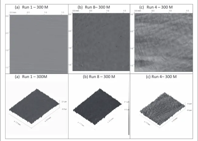
Figure3depicts typical 2 and 3-dimensional micrographies of 300M steel samples after electropolishing according to experimental design runs(runs 1, 4 and 8).

The topography of the surface has been considerably modified and surface roughness is reduced or increased according to the operating conditions. As observed infigure3(c), peaks and valleys are clearly observed. On the contrary, forfigure3(a) with a lower Ra value, the surface is flat due to a uniform dissolution. Similar profiles are observed for 4340 steel samples.

Figure 2. Surface responses:(a) dissolved thickness, (b) Ra for 300M Steel- with X3=+1.

Table 8. Compromise domain fulfilling the requirements for AISI 4340 and 300 M steels.

AISI 4340 300 M

Requirements Y1ò [15; 17]/μm Y2„0.06/μm Y3ò [15; 17]/μm Y4„0.06/μm

Xicombinations fulfilling each Yi X1ò [−1.00; −0.60], X1ò [−1.00; −0.40], X1ò [−1.00; −0.65], X1ò [−1.00; −0.9],

requirement(i=1 to 4) X2ò [0.74; 1.00], X2ò [0.60; 1.00], X2ò [0.75; 1.00], X2ò [0.84; 1.00],

X3=1.00 X3=1.00 X3=1.00 X3=1.00

Compromise domain fulfilling X1ò [−1.00; −0.60], X1ò [−1.00; −0.9],

Yiò [15; 7] with i=1;3 and X2ò [0.74; 1.00], X2ò [0.84; 1.00],

4. Conclusion

The electropolishing technique is a surface treatment that used to remove the metal surface rough irregularities without creation of internal stresses. The present study shows that AISI 4340 and 300M steel electropolishing can be achieved in a perchloric/acetic acid electrolyte using statistical methods. The effects of the operating conditions(current density, electrical charge, temperature) and electrolyte composition (Iron ions

concentration) are studied using two-level fractional factorial design (FFD). Using the sequential experiment strategies(i.e., the fractional factorial design), the factors and interactions for the EP process with the dissolved thickness and the roughness criterium(Ra) varying respectively from ca. 10.5 to 24.3 μm and 0.06 to 0.22 μm for AISI 4340 and from ca. 10.1 to 24.7μm and 0.04 to 0.19 μm for 300M steels are clearly demonstrated. The dissolved thickness and roughness criterium(arithmetic average of the absolute values (Ra)) are described using fitted models. Model validation using ANOVA analyses, check point-tests confirmed that the results are reliable and accurate. The predicted values obtained with models are in close agreement with the experimental data. As expected, these valuable results show that, dissolved thickness and Ra strongly depend on the polarization conditions(I and Q) effects for the two ferrous metals even if Iron ions concentration also affects the EP behaviors of steels. For all responses, the positive coefficients of X1(Q), X2(I), and X1X2indicate a constructive contribution and the negative coefficient of X3(Iron ions concentration), an antagonistic effect. Temperature (X4) has no effect in the domain studied.

The contour plots for the dependence of thickness and Ra on factors X1(electrical charge) and X2(current density) while keeping X3(Iron ions concentration) constant were constructed by using the regression model for each substrate. This allowed us to define a compromise zone where all the experimental responses fulfill the specifications imposed by the researchers to achieve the aims proposed, i.e. a dissolved thickness comprised between 15–17 μm and arithmetic roughness criteria less than 0.06 μm.

ORCID iDs

V Roscol https://orcid.org/0000-0002-5978-3308

W Bensalah https://orcid.org/0000-0003-2167-3936

M Depetris-Wery https://orcid.org/0000-0001-7997-9749

H F Ayedi https://orcid.org/0000-0002-3062-264X

References

[1] Spitalsky E 1910 German Patent 225873 [Original not available; cited by R. Pinner, Electroplating and Metal Finishing, 7 (1954) 295] [2] Jacquet P A and Figour H 1931 French Patent 707526

[3] McG Tegart W J 1959 The Electrolytic and Chemical Polishing of Metals in Research and Industry 2nd edn (Oxford: Pergammon P.) [4] Padamsee H 2009 RF Superconductivity: Volume II: Science, Technology, and Applications (New York: Wiley)

[5] Abbott A P, Ryder K S and König U 2008 Electrofinishing of metals using eutectic based ionic liquids Trans. IMF86 196–204 [6] Patil Y B and Dulange S R 2014 A review on electropolishing process and its affecting parameters international IJARSE 3 246–52 [7] Schwartz W 2003 Electropolishing Plating and Surface Finishing 3 8–12

[8] Chang S-C, Shieh J-M, Dai B-T, Feng M-S, Li Y-H, Shih C-H, Tsai M-H, Shue S-L, Liang R-S and Wang Y-L 2003 Superpolishing for planarizing copper damascene interconnects Electrochem. Solid-State Lett.6 G72_–4

[9] Landolt D, Chauvy P-F and Zinger O 2003 Electrochemical micromachining, polishing and surface structuring of metals: fundamental aspects and new developments Electrochimica Acta48 3185–201

[10] Huo J, Solanki R and McAndrew J 2005 A novel electroplanarization system for replacement of CMP Electrochem. Solid-State Lett.8 C33–5

[11] Suni I I and Du B 2005 Cu planarization for ULSI processing by electrochemical methods:a review IEEE Trans Semicond. Manufacturing 18 341–9

[12] Tajima K, Hironaka M, Chen K-K, Nagamatsu Y, Kakigawa H and Kozono Y 2008 Electropolishing of CP Titanium and its alloys in an alcoholic solution-based electrolyte Dental Materials J.27 258–65

[13] Lin C and Hu C 2009 Electropolishing of 304 stainless steel: surface roughness control using an experimental design and a summarized electropolishing model Surf. & Coatings Techno.204 448–54

[14] Yang G, Wang B, Tawfiq K, Wei H, Zhou S and Chen G 2016 Electropolishing of surfaces: theory and applications Surface Engineering 33 1–8

[15] Mohan S, Kanagaraj D, Sindhuja R, Vijayalakshmi S and Renganathan N G 2001 Electropolishing of stainless steel—a review Trans IMF.79 140–2

[16] Rokicki R and Hryniewicz T 2012 Enhanced oxidation-dissolution theory of electropolishing Trans IMF.90 188–96

[17] Shuo-Jen L, Yi-Ho C and Jung-Chou H 2012 The investigation of surface morphology forming mechanisms in electropolishing proces Int. J. Electrochem. Sci. 7 12495_–506

[18] Awad A M, Ghazy E A, Abo El-Enin S A and Mahmoud M G 2012 Electropolishing of AISI 304 stainless steel for protection against SRB biofilm, Surf. & Coatings Techno.206 3165–72

[19] Bonaccorso A, Schäfer E, Condorelli G G, Cantatore G and Trip T R 2008 Chemical analysis of nickel-titanium rotary instruments with and without electropolishing after cleaning procedures with sodium hypochlorite Journal of Endodontics34 1391–5

[20] Palmieri V 2003 Proc. of 11th Workshop on RF Superconductivity Travermünde paper WeT02

[21] Hryniewicz T, Rokicki R and Rokosz K 2008 Co-Cr alloy corrosion behaviour after electropolishing and magnetoelectropolishing treatments Mater. Lett.62 3073–6

[22] Bourscheid G and Bertholdt H 1990 How production technologies influence the surface quality of ultraclean gas-supply equipment Microcontamination 8 43–6

[23] Landolt D 1987 Fundamental aspects of electropolishing Electrochemica Acta32 1–11

[24] Datta M and Landolt D 2000 Fundamental aspects and applications of electrochemical microfabrication Electrochimica Acta45 2535–58

[25] Wang P 2011 Mechanistic study of copper electropolishing Ind. Eng. Chem. Res.50 1605–9

[26] Piotrowski O, Madore C and Landolt D 1998 The mechanism of electropolishing of titanium in methanol-sulfuric acid electrolytes J. Electrochem. Soc.145 2362–8

[27] Neelakantan L and Hassel A W 2007 Rotating disc electrode study of the electropolishing mechanism of NiTi in methanolic sulfuric acid Electrochimica Acta53 915–9

[28] Abbott A P, Capper G, Swain B G and Wheeler D A 2005 Electropolishing of stainless steel in an ionic liquid Trans. IMF83 51_–3 [29] Abbott A P, Capper G, McKenzie K J, Glide A and Ryder K S 2006 Electropolishing of stainless steels in a choline chloride based ionic

liquid: an electrochemical study with surface characterisation using SEM and atomic force microscopy Phys. Chem.8 4214_–21 [30] Lee S-J and Lai J-J 2003 The effects of electropolishing process parameters on corrosion resistance of 316 L stainless steel Journal of

Materials Processing Technology140 206–10

[31] Shigolev P V 1974 Electrolytic and Chemical Polishing of Metals 2nd edn (Israël: Freund Pub.) [32] Box E P, Hunter W G and Hunter J S 1978 Statistics for Experimenters (New York: Wiley) [33] Montgomery D C 1991 Design and Analysis of Experiments (New York: Wiley) [34] Goupy J 1999 Plans d’expériences pour surfaces de réponse (Paris: Dunod)

[35] Mathieu D and Phan Tan-Luu R 1997 Approche méthodologique des mélanges Plans d’expériences: Application à l’entreprise (Paris: Technip) 5

[36] Lewis G A, Mathieu D and Phan-Tan-Luu R 1999 Pharmaceutical Experimental Design (New York: Marcel Dekker)