Science Arts & Métiers (SAM)
is an open access repository that collects the work of Arts et Métiers Institute of
Technology researchers and makes it freely available over the web where possible.
This is an author-deposited version published in:
https://sam.ensam.eu
Handle ID: .
http://hdl.handle.net/10985/19543
To cite this version :
Charles FOULQUIÉ, Sofiane KHELLADI, Michael DELIGANT, Luis RAMÍREZ, Xesús
NOGUEIRA, Jacky MARDJONO - Numerical assessment of fan blades screen effect on fan/OGV
interaction tonal noise - Journal of Sound and Vibration - Vol. 481, p.1-20 - 2020
Any correspondence concerning this service should be sent to the repository
Administrator :
[email protected]
Numerical assessment of fan blades screen effect on fan/OGV
interaction tonal noise
Charles Foulquié
a,c, Sofiane Khelladi
a,∗, Michael Deligant
a, Luis Ramírez
b,
Xesús Nogueira
b, Jacky Mardjono
caArts et Metiers Institute of Technology, CNAM, LIFSE, HESAM University, F-75013, Paris, France bGroup of Numerical Methods in Engineering, GMNI, Universidade da Coruña, A Coruña, Spain cSafran Aircraft Engines, Rond-point René Ravaud, 77550, Reau, France
Keywords:
Aeroacoustics Turbojet fan noise Outlet guide vane Turbomachines Linearized Euler equations Screen effect
Fan
High order finite volumes
a b s t r a c t
This work deals with sound generation and transmission in a fan stage. The study is done on a subsonic Fan stage and interaction noise between the fan wakes and the Outlet Guide Vanes (OGV) is considered. For this purpose, the Linearized Euler Equations (LEE) are solved with a steady axisymmetric flow. The acoustic sources are modelled by a scattering approach. Numerical simulations are carried out in an unwrapped cylindrical layer using a high-order finite volume solver. In order to explicitly take into account the moving fan blades into the propagation medium, a high-resolution sliding mesh technique is used. The simulation results, which highlight the screen effect of moving fan blades on fan/OGV interaction tones, are consistent with analytical literature.
1. Introduction
The increase in the turbojet bypass ratio has resulted in the relative emergence of fan noise by comparison with other noise sources. On modern architectures, Fan noise is practically predominant at all operating engine speeds. Many aeroacoustic mech-anisms are at the origin of Fan noise. Their occurrence and their intensity are strongly correlated with the system configuration and the operating conditions. In particular in subsonic Fan stages, the interaction noise generated by the fan wakes impinge-ment on downstream Outlet Guide Vanes (OGV) is predominant. This source of noise has been widely studied using analytical, semi-analytical or more advanced numerical methods [1].
The increase in the turbojet bypass ratio has resulted in the relative emergence of fan noise by comparison with other noise sources. On modern architectures, Fan noise is practically predominant at all operating engine speeds. Many aeroacoustic mech-anisms are at the origin of Fan noise. Their occurrence and their intensity are strongly correlated with the system configuration and the operating conditions. In particular in subsonic Fan stages, the interaction noise generated by the fan wakes
impinge-∗
Corresponding author.
ment on downstream Outlet Guide Vanes (OGV) is predominant. This source of noise has been widely studied using analytical, semi-analytical or more advanced numerical methods [1].
The screen effect of fan blades rotation on acoustic waves generated by the fan/OGV interaction remains difficult to take into account outside analytical studies [2–6]. These works, which are theoretically useful to understand acoustic transmission through the fan stage, suffer from consequent limitations on the geometry representation and the flow intricacy. In most current numerical models, the screen effect is either neglected [7] or implicitly taken into account [8–10].
In the case of hybrid approaches based on acoustic analogies, the calculations are performed in two steps. In the first step, an unsteady CFD analysis is conducted to obtain the acoustic sources. In the second step, the propagation of acoustic waves from these sources is either modelled by a Green’s function [7] or calculated using a propagation operator [11]. As far as semi-analytical methods are concerned, the use of a suitable analogy [12] certainly allows us to take into account the effect of the rotating average flow (swirl). However, the formalism using analytical Green’s functions, in their usual form, does not allow to include the fan blades screen effect.
The numerical resolution of a propagation operator allows to reproduce sound propagation from sources through the fan. However, the use of a propagation operator with source terms involves the risk of counting some propagation effects several times, due to the lack of an adapted theoretical basis which permits the clean separation of the mechanisms of generation and propagation in the presence of swirling flow. Moreover, and beyond this consideration, the question of the stability of the operator arises. Despite these drawbacks, approaches based on acoustic analogies have been used in Ref. [10] for instance. In their work, the effect of the fan is not explicitly taken into account. Instead, the authors integrate in the source term all the mechanisms of generation and propagation inside the Fan-OGV stage.
An alternative to the approaches based on acoustic analogies is the direct resolution of Navier-Stokes equations. For obvious reasons of calculation cost, the “zonal” approach is considered in most cases. Simulations using Navier-Stokes equations are restricted to the Fan-OGV region, whereas the propagation inside the terminations (inlet/outlet), is taken into account by a non-viscous model. The connexions between the regions are done by using a mode-matching technique [8,9,13]. Using high-fidelity simulation of coupled Fan/OGV system [13], most of underlying physics is taken into account. In particular, it allows to capture both the screen effect of the fan on the acoustic waves and the feedback of acoustic waves on the fan wakes generation [1].
High-fidelity direct computation of radiated noise is still expensive and hypothesis on the flow can be done to make it more accessible [14]. Considering only the sound generation, Fan/OGV interaction tones are often modelled with inviscid flows [15–19]. The calculations can be carried out with linear equations when the hypothesis of small perturbations is verified [19,20]. Often, a non-linear computation is performed to take into account the nonlinear interactions due to the perturbations of large amplitudes [15–18]. A linearized viscous equation system has also been employed with no significant improvement in accuracy [21].
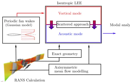
In this work we present a numerical strategy based on the linearized Euler equations (LEE) which explicitly takes into account the screen effect of the fan blades on the fan/OGV interaction tones. In the context of linearized approaches, a steady state simulation is required to characterize the mean flow field [21]. Here, we propose to use a RANS calculation with a mixing plane interface to characterize a theoretical average flow field which is supposed axisymmetric. This simulation is also exploited to extract speed deficits downstream of the fan. The obtained velocity profile feeds a Gaussian wake model which only accounts for the coherent part of the wake. In this type of computation, the vortical-mode scattering on the OGV vanes is usually calculated by convection of the perturbation. Here, in order to simplify the numerical implementation, the disturbance is imposed on the OGV by using a scattering approach based on the frozen gust assumption. No simplifying hypothesis were formulated on the geometry of the blades. The whole strategy of simulation is sketched inFig. 1.
The calculations are carried out in an unwrapped cylindrical layer of a representative fan stage for two subsonic operating points.1 The two dimensional approximation of the steady flow is done by assuming an equilibrium between the pressure and
the centrifugal forces along the cylindrical layer. The numerical simulation is done in the time domain by using a high-order finite volume solver based on Moving Least Squares (MLS) approximations. The relative motion between the fan blades and the OGV blades is handled through a high-resolution sliding mesh technique. A novel technique for considering periodic boundary conditions in turbofan simulations is also proposed.
The proposed approach aims to highlight some key mechanisms, often not discussed in the literature. It concerns the trans-mission of modes through a rotating blade cascade. An incident mode on a rotor experiences frequency and modal scattering where scattered modes can be regenerated at other harmonics of the blade-passing frequency (BPF) and orders shifted by a multiple of the blade number.
This paper is organized as follows. The modelling and the calculation procedure are presented in sectionII. The numerical method used to solve LEE in presence of rotating bodies and complex geometries is then briefly described in sectionIII. The last section presents the numerical simulations and the assessment of screen effect.
1The cylindrical layer is extracted at 80% of the fan leading edge radius. The study is done with 41% and 61% of the fan nominal rotation speed where 61%Nm nominal rotation speed corresponding to the “approach point”.
Fig. 1. Sketch of the simulation strategy.
2. Modelling and calculation procedure
2.1. Governing equations
In the propagation medium, the effect of viscosity is neglected and small perturbations are assumed (|
𝜌
′|≪ 𝜌
,|p′|≪
p), sothe linearized Euler equations (LEE) are used. The steady part of the flow is written as U=[
𝜌, 𝜌
v,
p]Tand the fluctuating part read as U=[𝜌
′, 𝜌
v′,
p′]T. The LEE equations written in conservative variables form read:⎧ ⎪ ⎪ ⎪ ⎨ ⎪ ⎪ ⎪ ⎩
𝜕𝜌
′𝜕
t + ∇ · (𝜌
v′+𝜌
′v)=0𝜕
(𝜌
v′)𝜕
t + ∇ · (𝜌
v⊗
v′+p′I)+(∇⊗
v)T· (𝜌
′v+𝜌
v′) =0𝜕
(p′)𝜕
t + ∇ · ( p′v+𝛾
v′)+ (𝛾
−1)(p′∇ ·v−v′· ∇(p))=0 (1) 2.1.1. Two-dimensional assumptionThe LEE system 1 is considered along a cylindrical layer of the fan-OGV stage. This two-dimensional analysis assumes that there is an equilibrium between the pressure and the centrifugal forces along the cylindrical layer. In other words, this approach is only valid for cases with no radial shifts of the meridional streamlines (for example configurations with constant hub and tip radius at the design point [22]). In a real fan stage, the angle of the spinner makes invalid this approach for low values of the radius. However, when the analysis is done for middle/high values of the radius of a conventional fan stage, the two-dimensional assumption remains acceptable.
The configuration investigated here is an industrial demonstrator of a conventional high bypass ratio fan OGV stage with a scale of 1∶2. As shown inFig. 2, the study is carried out on a cylindrical layer at 80% of the fan leading edge radius for two subsonic reduced speeds: 41% and 61% of the nominal rotation speed. Since the angle (
𝜑
) of the velocity of the steady flow is less than 5◦all along the axial direction in both operational points, the error introduced by the proposed approach is acceptable.2.1.2. Steady flow modelling
First, an axisymmetric modelling of the mean flow is done by averaging the flow in the azimuthal direction. Obviously, the two-dimensional assumption leads to neglect the radial component of the flow and the mean flow modelling reads:
Fig. 2. Fan-OGV geometry (courtesy of MAESTRO project of Safran Aircraft Engines). The cylindrical cut is made at 80% of the leading edge radius.
A uniform mean flow is considered in the axial direction all along the fan-OGV stage:
vz(z) =Vz (3)
The azimuthal component of the mean flow is assumed to be uniform inside of the fan region and equal to zero outside. A relatively weak gradient is applied to the interfaces between the regions using a hyperbolic tangent function. Finally the azimuthal component of the mean flow all along the fan-OGV stage is written as:
v𝜃(z) = V𝜃 2 ( tanh ( z−za ka ) −tanh ( z−zb kb )) (4)
where V𝜃is the uniform swirl component and za, zb, ka, kbare the hyperbolic tangent function parameters. The uniform swirl component of the mean flow V𝜃is modelled as a linear combination of a rigid body rotation and a free vortex [22] as
V𝜃= Ωfrc+ Γ∕rc (5)
whereΩfis the rotation speed of the fan,Γthe intensity of the free vortex and rcis the radius of the cylindrical layer. The parameters Vz,Γ, za, zb, ka, kbare obtained from a RANS simulation performed beforehand.
2.2. Source modelling
The acoustic sources are modelled in two steps. First, the fan wakes are approximated by using a Gaussian model. Then, in order to avoid computing the convection of the fan wakes, the scattering formulation of LEE equations is used to model the interaction noise generated by the fan wakes impingement on downstream OGV.
2.2.1. Wake modelling
We use a wake model initially proposed as part of an analytic methodology [23]. This model is based on the hypothesis that wakes are convected, incompressible and pressure-free. Furthermore, the incident speed deficit is modelled using a Gaussian distribution. The validity of this Gaussian modelling has been shown experimentally [24]. The wake of a fan blade k is defined as follows u′v,k=u0(z)exp { −
𝜉
( rc𝜃
+ Δ𝜃
(z) b(z) )2} e𝛽 (6)with
𝜉
= ln2. u0(z)and b(z)are the maximum deficit in the center of the wake and the half-width, respectively. Both of them are functions of axial position.Δ𝜃
(z) = z∕tan𝛽
is the azimuthal phase shift due to swirl.The vorticity field generated by the set of fan blades is expressed as an infinite sum of the elementary profile in which the azimuthal periodicity is introduced.Θ = 2
𝜋
∕B:u′v=
+∞
∑ k=−∞
Fig. 3. Fan-wakes modelling (cylindrical cut in the reference frame(z, 𝜃)).
The source model defined above must be fed by the functions describing the half-width of the wake b(z)and the maximum deficit in the center of the wake V0(z). In the set of calculations, we will consider a function b(z)as constant. The maximum deficit is modelled by a second Gaussian function centered on the leading edge of the OGV.
u0(z) =u0exp { −
𝜉
′ ( z−d b′ )2} (8)with
𝜉
′ = ln(2)and b′ = 0.
05. The distance between the leading edge of the stator blades and the half chord line of the rotor blades is given by d. The wake model and associated parameters are shown inFig. 3.2.2.2. Scattering formulation
The scattering formulation of LEE allows solving a problem of sound generation by a gust-airfoil interaction without comput-ing the convection of the gust. A major advantage of this formulation is that the treatment of boundary conditions is facilitated. The scattering formulation consists in rewriting the field of fluctuating velocities by separating the wakes velocity, denoted by u′
v, from the velocity field scattered by the OGV, denoted by u′a, as
v′=u′v+u′a (9)
By assuming that the wakes disturbances are solenoidal and convected with the mean flow (frozen gust assumption), this approach allows solving the system of equation(1)by considering only the scattered field [25], as follows
⎧ ⎪ ⎪ ⎪ ⎨ ⎪ ⎪ ⎪ ⎩
𝜕𝜌
′𝜕
t + ∇ · (𝜌
u′ a+𝜌
′v ) =0𝜕
(𝜌
u′ a)𝜕
t + ∇ · (𝜌
v⊗
u′ a+p′I ) +(∇⊗
v)T· (𝜌
′v+𝜌
u′ a) =0𝜕
(p′)𝜕
t + ∇ · ( p′v+𝛾
u′a ) + (𝛾
−1) ( p′∇ ·v−u′a· ∇(p) ) =0 (10)Using this system of equations, the scattered acoustic wave now originates from the boundary condition on the OGV. Note that the frozen gust assumption is valid only if the turbulence velocities are weak and the convected distance is not much greater than a blade chord, which is the case in the present study.2
By assuming that only velocity fluctuations normal to the OGV boundary are likely to interact with the OGV, the noise scattered on OGV from fan wakes disturbances can be computed. For this purpose we must consider that the total velocity on a point located on the OGV is given by v=v+u′
v+u′a. Since the normal component of the total velocity is zero (v·n = 0)
at the OGV boundaries and assuming that v·n=0 we obtain:
u′a·n= −u′v·n (11)
2In the present case, the turbulence is only a few per cent of the mean flow speed. Also, fan wakes are extracted from a RANS simulation at the mixing plane location which is located about one fan blade chord away from the OGV leading edge.
where n is a unit vector along the local normal of OGV boundaries and the wake velocity (u′
v) is given by the model introduced
in the previous paragraph.
Finally, the problem is to solve the system of equation(10)with the boundary condition on the surface of OGV prescribed by equation(11). It is important to note that this approach is exact only when a gust-plate interaction is considered. The compu-tation of noise radiated from a flat plate subjected to a normal incidence gust is proposed in theAppendix Aas a validation test case for this approach.
3. Numerical method
3.1. General framework
3.1.1. Finite volume discretization in ALE formulation
The finite volume formulation for LEEs in conservative form reads:
∫A
𝜕
U𝜕
t +H(U)dA= − ∮Γ (U) ·n dΓ (12)
where (U)is the flux matrix and the vector H(U)contains the refraction terms. (U) ·n is the normal flux crossing the
inter-cell boundary, A,Γand n are respectively the area, the contour and the normal to the control surface. In order to account for the relative motion of the rotor with respect to the stator, the sliding mesh technique is used. This technique requires the use of an Arbitrary Lagrangian-Eulerian (ALE) formulation. The equations are written in a reference frame which moves with the grid. The flux matrix (U)and the vector H(U)in ALE formulation read
(U) = ⎛ ⎜ ⎜ ⎜ ⎝
𝜌
v′+𝜌
′(v−v g)𝜌
(v−vg)⊗
v′+p′I p′(v−v g) +𝛾
pv′ ⎞ ⎟ ⎟ ⎟ ⎠,
H(U) = ⎛ ⎜ ⎜ ⎜ ⎝ 0 ( ∇⊗
v)T· (𝜌
′v+𝜌
v′) (𝛾
−1)(p′∇ ·v−v′· ∇(p)) ⎞ ⎟ ⎟ ⎟ ⎠where v and vgare, respectively, the mean flow velocity and the grid velocity at cell interface boundary. Note that the grid velocity vgis subtracted from the mean flow velocity v in the flux matrix, whereas the refraction vector H(U)remains unchanged.
3.1.2. Generalized Godunov-type scheme
The implementation of the finite volume method is done using a generalized Godunov-type scheme. This kind of scheme can be broken down into two stages: the “projection” stage, which is exclusively of numerical nature and the “evolution” stage which holds the physics.
In the original Godunov’s scheme [26] the projection stage is ensured by a piecewise constant approximation of the variables. Of course by doing a piecewise constant approximation (cell averages), part of the knowledge of the original initial data is lost. Thus, the original Godunov’s method, which is only first order accurate in space and time, introduces excessive numerical dissi-pation. To address this problem, a high-order extension of Godunov-type finite volume method is needed. The key ingredient in this type of scheme is the piecewise polynomial approximation. Here, Moving Least Squares (MLS) [27] approximations are used for the computation of a high order accurate piecewise polynomial approximation. For the sake of brevity, this approximation is shown inAppendix B.
The evolution step consists in resolving the Riemann problem at each integration points of inter-cell boundaries (Flux com-putation). The solution can be computed exactly as long as the governing equations are linear. Thus, the flux reads as follows
(U−
,
U+) ·n=1 2 ( (U−) + (U+))·n−1 2 4 ∑ k=1𝛼
k|𝜆
k|ek (13)where−and+refers respectively to the “left” and “right” Riemann states of the inter-cell boundaries. ekand
𝜆
kare theeigenvec-tor and the eigenvalues of the flux Jacobian [28] respectively.
𝛼
krepresent the wave strengths along the eigenvector direction. In the special case of grid motion, the set of eigenvalues becomes𝜆
1= (v−vg) ·n+c, 𝜆
2= (v−vg) ·n−c, 𝜆
3=𝜆
4= (v−vg) ·n (14)The wave strengths and the eigenvectors remain unchanged with respect to a static mesh formulation.
3.1.3. Semi-discretized form and mass matrix inversion
The complete process of spatial discretization (flux quadrature, volumic term discretization) is not described here for the sake of brevity. Readers can refer to Refs. [29] for more details. Let’s assume that the spatial discretization leads to the following
Fig. 4. Halo-cell method for flux computation. system: M· (
𝜕
U𝜕
t −H(U) ) =R(U) (15) where U= [U1,
…,
UN]T, H= [H(U1)
,
…,
H(UN)]T, R(U) = [(U1),
…,
(UN)]Tis the residual matrix and M is the mass matrix.System 15 is the semi-discretized form of system 3.1.1.
Using an explicit time integration scheme, it is required to compute the inverse of the mass matrix to solve the system
𝜕
U𝜕
t =M−1R(U) +H(U) (16)
In general, a diagonal structure is recovered by enforcing reconstructions that preserve the mean. But this technique induces a loss of accuracy of the reconstructed variables, and it is not suitable for very high-order reconstructions [30]. This is why we prefer to be as accurate as possible even though this procedure leads to solve a system with non-diagonal mass matrix, which is more expensive in terms of computation time.
The inverse matrix can be computed by using a low-complexity approximation which consist in: (i) rewriting matrix M as the subtraction of the matrix of perturbation E from the identity matrix I and by (ii) using the Neumann series [31]:
M−1= (I−E)−1= pInv ∑
k=0
Ek+o(pInv) (17)
The convergence criteria of this series expansion is verified as long as the spectral radius of the matrix E is less than unity (
𝜌
(E) =𝜆
max(E)<
1).3.1.4. Time integration
Time integration is performed by using a low storage five-stages fourth-order explicit Runge-Kutta scheme [32]. This scheme has a wider stability region than a standard explicit fourth-order Runge-Kutta scheme which allows using larger time steps.
3.2. Boundary conditions 3.2.1. Sliding mesh technique
In order to account for the relative motion between rotor and stator, here we use the sliding mesh technique proposed in Ref. [33]. In this technique, a halo-cell (or ghost-cell) is created as a mirror image of a given cell I. This is schematically presented inFig. 4. In order to solve the Riemann problem between the halo-cell and the cell I, it is required to compute the value of the variables at the centroid of the halo-cell, so that the mean is preserved. In order to do that, a MLS approximation is performed at the position of the halo cell. MLS-shape functions are computed by using the stencil of the closest cell. This technique induces an error of mass conservation, but numerical experiments have shown that this error is of the same order of magnitude as the error in the variables when a fixed grid approach is used and the order of accuracy of the numerical scheme is preserved [33]. This approach avoids the computation of intersections used by most of the sliding mesh approaches, which introduces additional complexity in the coding and a high computational cost.
We refer the interested reader to Ref. [33] for a complete description of the sliding mesh technique used in this work.
3.2.2. Natural periodic boundary conditions
Periodic boundary conditions are very useful in many situations where the geometry of the simulated problem has a certain periodicity. When dealing with large stencils (which is the case of high-order MLS stencils), the implementation of a peri-odic boundary condition is not straightforward [34]. When sliding meshes and periodic boundaries are considered together, the implementation becomes more complex. Here, we propose a simple workaround which consist in wrapping up the plane domain to a cylinder. Thus, the periodic boundary condition is naturally ensured. Actually, there is no more periodic interface:
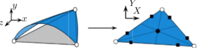
Fig. 5. Close up to facet and real face on cylinder quadrature points (▪), element centroid (•) and element nodes (◦).
the cells connections are natural. This means that there is no special requirement on the mesh for creating the linear interface. Wrapping rectangular plane domain into a cylinder allows us to take into account periodic domain with a linear sliding interface. The 3D cylinder and 2D unwrapped plane geometry are parametrized as
⎧ ⎪ ⎨ ⎪ ⎩ x=rccos
𝜃
y=rcsin𝜃
z⏟⏞⏞⏞⏞⏞⏞⏞⏟⏞⏞⏞⏞⏞⏞⏞⏟
⟹ { X=rc𝜃
[2𝜋
] Y=z⏟⏞⏞⏞⏞⏞⏞⏞⏞⏞⏟⏞⏞⏞⏞⏞⏞⏞⏞⏞⏟
3D cylinder geometry 2D unwrap plane geometry
(18)
This 3D cylinder surface geometry is easily created, meshed and exported. All cells are discretized facets of the cylinder. All exported points are on the surface of the cylinder with coordinates verifying the left part of (18). In order to avoid adding discretization errors due to the curvature of the surface, the area of each cell is considered as the area of the cell on the cylin-der surface (seeFig. 5). This area is computed using the{X
,
Y}variables. The positions of the cell centroid, face centroid and integration points are also computed to be on the cylinder surface. In order to compute the MLS shape functions it is required to determine the distance dA→B, between two points A = XA,
YAand B = XB,
YB. In the curved surface, this distance can be computed as ΔXA→B=rcsign(𝜃
B−𝜃
A)min { |𝜃
B−𝜃
A|,
|𝜃
B−𝜃
A−2𝜋
| } (19) ΔYA→B=zB−zA (20) dA→B= √ (ΔXA→B)2+ (ΔY A→B)2 (21)3.3. Numerical validation of the method
The purpose of this section is to test the accuracy of the numerical method. In particular, the order of accuracy of the method is monitored on a cylindrical computational domain with a sliding interface.
3.3.1. Test case description
The problem concerns the propagation of a Gaussian pulse in a medium at rest (without flow) through the reference domain
=x∈ [−l∕2
,
l∕2] ×y∈ [−L∕2,
L∕2]. In what follows, all variables are made non-dimensional by c(ambient sound speed) for the velocity scale,𝜌
(ambient density) for the density scale,𝜌
c2for the pressure scale,Δfor the length scale andΔ∕c for the timescale. The Gaussian pulse is introduced in non-dimensional LEE (
𝜌
=1, c=1, p=1∕𝛾
) by initializing the vector of conservative variables as following: Ux,y,t=0=𝜖
e− ln2 b ( 𝛿x2+𝛿y2) [1,
0,
0,
1]T (22)where
𝛿
x = x − x0,𝛿
y = y − y0and (x0,
y0) is the Gaussian impulsion location. b and𝜖
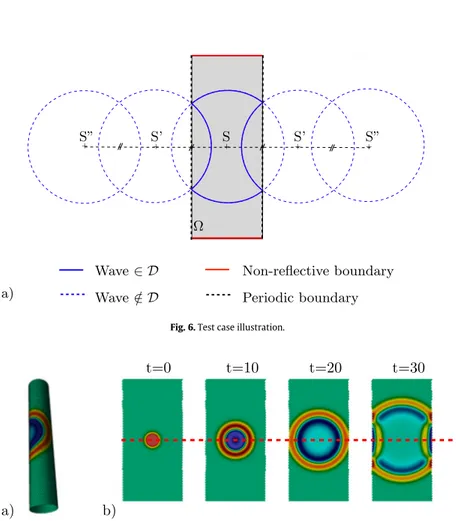
are respectively the half-width and the amplitude of the Gaussian pattern.As shown inFig. 6, the reference domain has periodic boundaries conditions at the borders x = ±l∕2 and non-reflecting ones at the borders y = ±L∕2. The impulsion is set at its center (x0 = 0
,
y0 = 0). This means that when the acoustic wave front reach the periodic boundaries a symmetric wave front enter the domain. The analytical solution of this test case is given by: p′ exact(x,
y,
t) = +∞ ∑ i=−∞ p′ gi(𝛿
x+l×i, 𝛿
y,
t) (23) with p′igthe analytical of a Gaussian impulsion alone: p′ gi(x
,
y,
t) =𝜖
2𝛼
∫ ∞ 0 exp(−𝜁
2 4𝛼
)cos(t𝜁
)J0(𝜁
r)𝜁
d𝜁
(24)Fig. 6. Test case illustration.
Fig. 7. 2D cylindrical computation with non-conform sliding interface (𝜔 =0.05): a) wrapped domain (t=15), b) unwrapped domain (t=0, 10, 20, 30), sliding interface location.
where J0is the Bessel function of the first kind and order zero, r=√
𝛿
x2+𝛿
y2. Please consult [35] for details and mathematicalproof.
The computational domain is obtained by wrapping the plane domain of referencer=x∈ [−l∕2
,
l∕2] ×y∈ [−L∕2,
L∕2]into the y-direction. The resulting domainc=
𝜃
∈ [−𝜋, 𝜋
] ×y∈ [−L∕2,
L∕2]is a cylinder with a radius of rc = l∕2𝜋
. Note that the cylindrical domain has a circular sliding interface located at y = 0. This way, the computational grid is decomposed into two parts: a fixed grid for the inferior part (y<
0) and a sliding grid for the superior part (y>
0) which rotates around its center with a non-dimensional rotational velocity𝜔
. Since the rotation is not physical, the acoustic wave must propagate through the sliding grid without any alteration. The computational configuration is shown inFig. 7.A cubic polynomial reconstruction (p = 3) is used with the purpose of reaching the 4th order of accuracy. The convergence study is performed on unstructured grids and the comparison with analytical solution is done at time tc = 30. The angular velocity of the sliding grid is set at
𝜔
= 0.
05. The time-step is set atΔt = 4.
0·10−1for each computation.3.3.2. Test case results
In order to quantify the numerical method accuracy, we define the local error at the center of an element of the mesh(
𝜃
i,
yi)at time tcas
𝛿
p′i=p′num(rc𝜃
i,
yi,
tc) −p′exact(xi,
yi,
tc) (25)The error norms L1, L2and L∞are defined as
L1= 1 A N ∑ i=1 Ai|
𝛿
p′i| L2= 1 A √ √ √ √∑N i=1 (Ai𝛿
p′i)2 L∞=max(|𝛿
p′i|) (26)Fig. 8. Accuracy curves for unstructured cylindrical grids with sliding interface. Test case parameters:𝜔 = 0.05, tc =30, b = 3,𝜖 = 1, l = 25, L =50; FV-MLS
parameters: p=3, nadd =4,𝜅=5, pi =1,Δt=4.0·10−1.
Table 1
Accuracy values for unstructured cylindrical grids with sliding interface. Test case parameters:𝜔 =0.05, tc =30, b=3,𝜖=1, l=25, L=50; FV-MLS parameters: p=3, nadd=4,𝜅=5, pi=1,Δt=4.0·10−1. k N h(k) L(k) 2 𝛼 (k) 2 L (k) 1 𝛼 (k) 1 L (k) ∞ 𝛼∞(k) 1 676 2.72 1.87·10−2 0 1.23·10−2 0 7.26·10−2 0 2 900 2.36 1.49·10−2 1.59 9.84·10−3 1.57 6.16·10−2 1.15 3 2288 1.48 5.14·10−3 2.28 3.1·10−3 2.47 2.8·10−2 1.69 4 4206 1.09 2.06·10−3 3.00 1.17·10−3 3.21 1.07·10−2 3.16 5 8218 0.78 5.49·10−4 3.95 3.04·10−4 4.02 3.03·10−3 3.76
where Aand Aiare respectively the surface of the whole domain and the surface of the element i. The point-by-point order of convergence
𝛼
∗(k+1)based on the L∗-norm which is computed from mesh resolution (k) and (k-1) is defined as:L(k)∗ = ( h(k) h(k−1) )−𝛼∗(k) L(k−1)∗ (27)
where h(k)is the characteristic element size of mesh resolution (k) and is given by h(k)=√A
∕N(k). The convergence curves and
values of the three error norms are given inFig. 8andTable 1. This study show both the validity of the approach and the high order of accuracy of the method. Readers can refer to Refs. [29,33] for more detail studies of the FV-MLS method in presence of sliding interface.
4. Numerical simulations and analysis of results
4.1. Numerical setting
The calculations are done at 80% of the fan leading edge radius of a representative fan stage designed by Safran Aircraft Engines. This fan stage has non-trivial common divisors between the number of fan blades (B=24) and the number of OGV blades (V=30). The greatest common divisor is gcd(B
,
V) =6. As a result, by introducing a periodicity condition in the com-putational domain, a simulation can be conducted on a reduced sector of angle𝜃
=𝜋
∕3. As shown schematically inFig. 9, the resulting cylinder sector of angle𝛼
=𝜋
∕3 and radius rcis wrapped into a full cylinder of radius r′c=2
𝜋
∕𝛼
×rc. This way anatural periodic condition appears. Note that the angular rotational velocity of the FanΩfshall be replaced byΩ′f=rc∕r′c× Ωf.
The sliding interface is located halfway between the fan and the OGV. The transfer of information through the interface is ensured by the method of the ghost cell [33]. Sponge zones upstream and downstream are used to dissipate some of the energy and thus avoid spurious reflections of the waves leaving the domain. In order not to compute the fan wakes convection into the simulation, the computation is carried out with the scattering formulation. Thus, the wakes speed deficits are applied directly to the skin of the OGV. Finally, reflective boundary conditions are used to model the action of fan blades on the acoustic mode. A sketch of the computational domain and the setup of the problem is shown inFig. 10.
The computational domain is divided into triangular element and a cell-centered configuration is adopted. The cylindrical computational mesh used for the computation is shown inFig. 11. The FV-MLS method is used with a cubic polynomial recon-struction (p=3) in order to reach the 4th order of accuracy. The number of elements of the computational mesh and the time step used depend on the engine speed. Thus, for the 41%Nm regime we choose N%13·103 elements and dt=3
.
5·10−3ms,whereas we choose N%23·103elements and dt=1
.
8·10−3ms for the 61%Nm regime.In order to study separately the effect of the swirl effect and the screen effect, the calculations were carried out on three configurations (seeFig. 12). In the first configuration we consider the OGV alone with axial flow (“OGV-axial”). In the second
Fig. 9. Natural periodicity condition by wrapping the calculation domain; Reduced computational domain a) Before transformation (cylinder sector of angle𝛼 = 𝜋∕3, radius rc, height h and angular rotational velocity of the sliding partΩf), b) After transformation (full cylinder of radius r′c =2𝜋∕𝛼× rc, height h and reduced angular
velocity of rotation of the sliding partΩ′f =rc∕r′c× Ωf).
Fig. 10. Schematic view of the flow and boundary conditions.
configuration, the OGV is considered alone with swirling flow (“OGV-swirl”). Finally, we consider the Fan-OGV with swirling flow (“FAN-OGV-swirl”).
4.2. Time-domain results
In this part, the results are presented in the time domain. First,Fig. 13presents a 360◦visualization of the pressure field in the FAN-OGV-swirl configuration for the two regimes 41%Nm and 61%Nm. This representation of the results is obtained by partially unwinding the computational grid so that it matches the curvature of the cylindrical layer of radius rc. Then, the domain 360◦ is reconstructed by reproducing the periodic pattern as many times as necessary (6) with the appropriate azimuth offset (
𝜋
∕3). Using this visualization, the acoustic screen effect appears important whatever the rotation regime.In order to analyse the pressure field, it is preferable to visualize the unrolled surface. In theFig. 14, the results are exposed for the 41%Nm regime by displaying the half (angle sector 180◦) of the cylindrical surface.
The OGV-axial configuration shows that some coherent wave fronts stand out. These wave fronts or azimuthal modes (m) can be numbered according to their orientation3 and number of pressure variation cycles (on 360◦in the azimuthal direction)
that compose them. By adopting this convention, one easily finds on the OGV-axial configuration at 41%Nm regime the modes
m = −6 and m = +18 propagating upstream of the OGV grid. At first sight, the presence of the tangential flow seems to cut out the mode m = +18 on the one hand (seeFig. 14-OGV-swirl−41%Nm) and the addition of the fan (seeFig. 14-FAN-OGV-swirl
−41%Nm) appears to disturb the wave fronts considerably.
3positive (+) if n·u
Fig. 11. View of the computational mesh used for the 61%Nm regime (N=23·103).
Fig. 12. The three different configurations selected for the study: a) OGV-axial, b) OGV-swirl, c) FAN-OGV-swirl.
Moreover, the checkerboard patterns shown inFig. 14illustrates clearly the interference between oblique waves of opposite rotation when unwrapped as two-dimensional maps. For instance, the Fan-OGV-swirl configuration seems to regenerate the mode m = +18 compared to the OGV-swirl configuration.
It can be seen from theFig. 15, with the same colour scale thanFig. 14, that the radiation structure for the 61%Nm regime is equivalent to that of the 41%Nm regime. The wave fronts are simply narrower and their inclination larger. The swirl and screen effects detected for the 41%Nm regime also appear in this configuration. Notice that the cut-off of the mode m= +18 does not occur anymore.
Fig. 13. Domain reconstruction 360◦(FAN-OGV-swirl configuration); visualization of the pressure at time t=10 ms for the two engine speeds: a) 41%Nm, b) 61%Nm. Cut radius rc =0.8·R.
Fig. 14. Results of acoustic pressure for 180◦in the unwrapped cut for the 41%Nm regime. From left to right: OGV-axial, OGV-swirl and FAN-OGV-swirl configurations. Cut radius at rc =0.8·R.
Fig. 15. Results of acoustic pressure for 180◦in the unwrapped cut for the 61%Nm regime. From left to right: OGV-axial, OGV-swirl and FAN-OGV-swirl configurations. Cut radius at rc =0.8·R.
In order to quantify the screen effect, the acoustic levels for the OGV-swirl and FAN-OGV-swirl configurations were calculated for three distinct azimuthal positions: a) upstream of the fan, b) between the fan and the OGV, c) downstream of the OGV.
Fig. 15also points out that at higher rotational velocity and corresponding axial-flow speed, the same modes are farther beyond the cut-off limit because their driving frequency increases, this is associated to shorter wavelength and smaller wave-front angles with respect to the vane-cascade wave-front.
The results are compiled inFig. 16. The average azimuthal acoustic level upstream of the fan is reduced by 1.6 dB for the 41%Nm regime and by 4.3 dB for the 61%Nm regime. Notice that sound is clearly increased downstream at 61%Nm regime.
The observation is limited because the superposition of acoustic modes makes it difficult to identify and quantify the physical mechanisms. A modal analysis is necessary in order to better analyse the evolution of the modal signature from one configura-tion to another.
4.3. Frequency-domain results
As it has been observed on the pressure field p(x
, 𝜃,
t), the response is not only periodic in time, but also periodic in the azimuthal direction. For a given axial position, the acoustic pressure, computed at Ntinstants samples a time interval T = k∕BPFand N𝜃angular positions, sampling a spatial intervalΘ = 2
𝜋
. Thus, the acoustic pressure can be decomposed using a Fourier series in space and time. This transform provides a representation of the solution as a function of the harmonic (n) and the azimuth modes (m) for each axial position (x):Pmn(x) = 2 N𝜃Nt N∑𝜃−1 l=0 N∑t−1 j=0 plj(x)exp ( −i2
𝜋
nj Nt ) exp ( −i2𝜋
ml N𝜃 ) (28)where plj(x)and Pmn(x)are the contractions of p(x
, 𝜃
l,
tj)and P(x,
m,
n). Moreover, n = 0,
…,
Nt∕2 and−N𝜃∕2<
m<
N𝜃∕2. Finally, the Fourier series in space and time allows to know the amplitude of each elementary wave, defined by its harmonic nFig. 16. Comparison of acoustic sound pressure levels on three successive cross sections ((a) z=20 mm, (b) z= −10 mm, (c) z= −40 mm) and for each regime; 41%Nm (left) and 61%Nm (right). FAN-OGV-swirl OGV-swirl.
Fig. 17. Modal analysis along the z-axis for the blade passing frequency (n =1) and the first two harmonics (n=2,3): a) 41% Nm regime, b) 61% Nm regime.
and its azimuth mode m, according to the axial position x. The results of the modal analysis as a function of the axial position z for each regime and each configuration are presented inFig. 17.
The tonal interaction noise resulting from the interaction mechanism between a rotor and a stator (both homogeneous) is modelled analytically by Tyler-Sofrin’s rule [36]. This rule, verified experimentally, predicts the modal structure of the radiated noise. According to it, the excited azimuthal modes are:
m=nB−lV (29)
where B and V are respectively the number of fan blades and the number of OGV blades, n is the harmonic of the blade passing frequency (BPF) tone and l∈ℤis an arbitrary integer. This result can be interpreted as a phenomenon of interference between the phase-shifted pressure fields coming from each OGV blade.
Fig. 18. Distribution of acoustic energy on mode-harmonic diagram(m,n)at the axial location z=0 mm and 41%Nm regime for configuration: a)OGV-axial, b)OGV-swirl. The expected position of Taylor and Sofrin’s modes are spotted by a circle on the diagram. The “V-shape” cut-off limit is represented by red lines. Colour scale is arbitrary in this illustration. (For interpretation of the references to color in this figure legend, the reader is referred to the Web version of this article.)
As shown inFig. 17, the computed modal signature respects the Tyler-Sofrin’s rule (hot colors correspond to dominant modes). Considering the OGV-axial configuration, we find in particular the dominant mode m = −6 which propagates at the blade passing frequency (n = 1) that have been previously identified on the time-domain results. The screen effect on this mode is even more important than the effect of swirl. Indeed, we note for both rotation regimes a very clear decrease in amplitude around the fan (configuration FAN-OGV-swirl). Whatever the configuration considered, the interaction mode m = +24, which is generated at the blades passing frequency (n = 1) is cut-off. Cut-on modes of higher harmonics (m = −12, m = +18,
m = −18, m = +12) are all affected by swirl on the one hand and by the screen effect on the other hand:
1. The mode m = −12 (n = 2) behaves independently of the regime and very similarly to the mode m = −6 (n = 1). 2. The mode m = +18 (n = 2) is cut-off by the swirl for the 41%Nm regime while remaining cut-on in presence of swirl for
the 61%Nm regime. This mode is then, independently of the regime, fed by the fan.
3. The mode m = −18 (n = 3) is not affected by the swirl and a reflection mechanism on the fan is visible for the 41%Nm regime. Considering the 61%Nm regime, the mode m = −18 is fed by the swirl.
4. The mode m = +12 (n = 3) has a very low intensity for the first two configurations. The amplitude of the mode increases as the fan passes for 41%Nm regime while remaining stable for the 61%Nm regime.
4.3.1. Cut-off condition and swirl
The azimuthal interaction modes are generated at the harmonic of the blade passing angular frequency nBΩfwith a speed
of rotation nBΩf∕m. The cut-off condition can be expressed as a function of the relative Mach number of the spinning mode Mrm
[37,38] which is defined as:
Mrm= √
Mz2+(M𝜃+Mm )2
<
1 (30)where Mz=Vz∕c is the axial Mach number, M𝜃=V𝜃∕c is the maximum azimuthal Mach number and Mm=nBΩfrc∕mc is the
absolute Mach number of the spinning mode. The mode is cut-off if the relative Mach number of mode Mrmis subsonic4(Mrm
<
1) [37,38].TheFig. 18-a) shows the classical mode-frequency diagram for the OGV-axial - 41%Nm configuration. The branches of the “V-shape” (which are based on the cut-off relation 30) point the limits of the cut-off zone (outside the “V”). For example, the interaction mode m = +24 (n = 1) which is outside the “V” is cut-off. Note that in pure axial flow (M𝜃 = 0) the branches of the “V-shape” are symmetric.
In accordance with the cut-off relation 30, a mode close to a branch turns from cut-on to cut-off or vice versa because of the swirl, depending on its either co-rotating or contra-rotating spinning phase. This is the case of the mode m = +18. As shown inFig. 18-b), in the presence of swirl the “V-shape” rotates counter-clockwise around its apex and the mode m = +18 turns from cut-on to cut-off. This way, the present numerical results in both OGV-axial and OGV-swirl are consistent with the cut-off relation 30. Note that the relative Mach number of spinning modes increase for the 61%Nm regime and the mode m = +18 remains cut-on in the presence of swirl.
4.3.2. Fan blades screen effect
The computed modal signature highlight two distinct mechanisms: a frequency and modal scattering and a reflection mech-anism. The frequency and modal scattering of the rotor is known to obey to a simple relationship. The incident azimuthal modes nB − lV which are generated at the harmonic of the blade passing angular frequency nBΩfare regenerated in scattered
azimuthal modes(n + 1)B − lV at associated angular frequencies(n + 1)BΩf. A detailed analysis has been published in a report by Hanson [39].
4Note that the converse of this assertion is not true: A supersonic relative Mach number is a necessary but not a sufficient condition allowing a mode to be cut-on.
Fig. 19. Frequency and modal scattering of the mode m = −6(n=1) into the mode m= +18(n=2) for the 41%Nm regime. FAN-OGV-swirl OGV-swirl.
Fig. 20. Reflection mechanism for modes m= −18 at 41%Nm regime (top) and m= −12 at 61%Nm regime. FAN-OGV-swirl OGV-swirl.
As shown inFig. 19, the scattering rule makes the mode m = +18 indeed expected at 2BPF(n = 2) from the mode m = −6 at BPF(n= 1) in both configurations. It should be noted that at 41%Nm regime the mode m = +18 (which is cut-off in the presence of swirl) turns cut-off to cut-on in the fan region because of the swirl reduction. Considering the fundamental frequency (n = 1) and the first harmonic (n = 2),Fig. 17actually evidences behaviour expected from basic mode/frequency scattering.
Following the scattering mode/frequency scattering rule, the mode m = +12 is also expected at 3BPF (n = 3) from the mode m = −12 at 2BPF (n = 2). This is the case for the 41%Nm regime but not for the 61%Nm regime. This difference between the two configurations is not well understood. It may be due to a limited time resolution for the 61%Nm regime that does not capture well the higher frequencies.
Secondly, we identify a reflection mechanism of less magnitude for the modes m = −18 and m = −12.Fig. 20illustrates this mechanism for both regimes.
5. Conclusion
In this paper, a numerical strategy to investigate the fan’s screen effect on fan/OGV interaction tones was proposed. This strategy is based on the resolution of the two-dimensional linearized Euler equations in presence of axisymmetric swirling mean flow. To assess the source mechanism a scattering approach based on a fan wake model was employed.
Time-domain simulations were carried out on an unwrapped cylindrical layer using a high-order finite volume method based on Moving Least Squares approximations. The relative motion between the fan blades and the OGV blades was modelled using a high resolution sliding mesh technique.
The numerical results showed that the acoustic signature is clearly impacted by the presence of the fan in the computational domain. The modal analysis highlighted for the blade passing frequency (BPF) and the first harmonic the existence of key mech-anisms: Tyler and Sofrin’s modes experiences frequency and modal scattering where scattered modes are regenerated at other harmonics of the blade-passing frequency (BPF) and azimuthal orders shifted by a multiple of the fan blade number.
The obtained two-dimensional results are in accordance with analytical literature and they should not be fundamentally questioned when going to three-dimensional computations (only quantitatively modified). In spite of that, three-dimensional calculations are needed to reinforce the conclusions of this study. These calculations will also make it possible to analyse the behaviour of radial modes through the fan stage, which are a first concern in designing UHBR turbofans.
CRediT authorship contribution statement
Charles Foulquié: Writing - original draft, Conceptualization, Methodology, Software. Sofiane Khelladi: Conceptualization,
Methodology, Software, Supervision, Writing - review & editing. Michael Deligant: Software, Validation, Writing - review & editing. Luis Ramírez: Visualization, Investigation. Xesús Nogueira: Writing - review & editing. Jacky Mardjono: Supervision.
Declaration of competing interest
The authors declare that they have no known competing financial interests or personal relationships that could have appeared to influence the work reported in this paper.
Acknowledgements
Xesús Nogueira and Luis Ramírez acknowledge the support given by FEDER funds of the European Union, Grants #DPI2015-68431-R of the Ministerio de Economía y Competitividad and #RTI2018-093366-B-I00 of the Ministerio de Ciencia, Innovación y Universidades of the Spanish Government, and by the Consellería de Cultura, Educación e Ordenación Universitaria of the Xunta de Galicia (program Axudas para potenciación de grupos de investigación do Sistema Universitario de Galicia 2018, grant #ED431C 2018/41).
Appendix A. Radiation from a flat plate subjected to a normal incidence gust
Let us consider the interaction between a x-direction flat plate airfoil of length l and a normal sinusoidal gust convected with the mean flow v= (u
,
0). The flow velocity in the x-direction is given by u=M×c and the gust is defined as follows:v(x) =
𝜖
cos(kxx−𝜔
t) (31)where
𝜖
is the gust amplitude, kxis the wave number in the x-direction. The frequency of the gust is directly related to the wave-number in the x-direction through Taylor’s hypothesis, as𝜔
= u × kx.Let us now write the LEE in conservative variables form in this specific case (uniform mean flow in the x-direction):
(U) = ⎧ ⎪ ⎪ ⎪ ⎨ ⎪ ⎪ ⎪ ⎩ d
𝜌
′ dt +𝜌
∇ ·v ′=0 d𝜌
v′ dt + ∇(p ′) =0 dp′ dt +𝛾
p∇ ·v ′=0 (32)where U= [
𝜌
′, 𝜌
v′,
p′]Tis the vector of conservative variables and d dt =𝜕 𝜕t +u
𝜕
𝜕xis the convective derivative.
Starting from these equations, the field of fluctuating velocities is rewritten by separating the incident gust velocity, denoted by u′
v= (0
,
v(x)), from the velocity field scattered by the plate, noted as u′a= (u′,
v′). Thus, we write: v′=u′v+u′a (33)
Since the gust is solenoidal and convected by the mean flow as a “frozen” pattern, it is possible to write the two following equations: ∇ ·u′ v=0 (34) du′ v dt =0 (35)
By substituting the decomposition of the field of fluctuating velocities 33 into the LEE system 32 and by using identities 34 and 35, we obtain: (Ua) = ⎧ ⎪ ⎪ ⎪ ⎨ ⎪ ⎪ ⎪ ⎩ d
𝜌
′ dt +𝜌
∇ ·u ′ a=0 d𝜌
u′ a dt + ∇(p ′) =0 dp′ dt +𝛾
p∇ ·u ′ a=0 (36)Identifying(U)and(Ua)means that the scattered field is only considered in the system of equationsand its originates
from the boundary condition on the flat plate airfoil [25]. It is in this sense that this method is called “scattering formulation”. To compute the noise scattered on the flat plate from gust disturbances, one has to look at the expression of total velocity:
v=v+ui+us= (u+u′
,
v′+v(x)) (37)By exploiting the nullity of the normal component of the total velocity on the wall (v·n = 0), the boundary condition to apply follows as
v′= −v(x) (38)
This validation case is carried out considering a length of the plate l equal to 1 m. The Mach number of the mean flow is 0
.
5 while the relative amplitude of the gust𝜖
is set to 0.
02. In order to address a non-compact plate case (𝜆
gust = 2𝜋
∕kx ≃ l) theaxial wave number kxis set to 6 m−1. To reach the steady-state more quickly the incident gust is introduced gradually using the
factor(1 − et/𝜏).
The computational domain is reduced to a half disk using the symmetry along the x-direction. It is divided in two parts: the physical zoneΩu = [0
, 𝜋
] × [0,
r1]and the sponge zoneΩs = [0, 𝜋
] × [r1,
r2]which is added to dissipate the energy ofacoustic waves before waves fronts reach the boundary. The total number of element is noted N.
We introduce the characteristic element size h to give a local measure of the mesh refinement. The characteristic element size on the plate is defined as hp = Np∕l with Npthe number of element along the plate, whereas the characteristic element
size on a half-circle at constant radius riis defined as hr
i =Nri∕
𝜋
riwith Nri the number of element along the half-circle. Thesimulation parameters and the computational domain are shown inFig. 21.
Fig. 21 Computational domain: r1 =5l, r2 =7l. Numerical parameters:Δt= 2.0e−5s,CFL=0.68,N= 18700, Physical zone (Ωu): hp ≃ 0.01,
hr1≃0.13𝜒=1.05, Sponge zone (Ωs): hr1≃0.13, hr2≃0.324𝜒=1.1. Gust’s parameters:𝜖= 0.02, M =0.5, kx =6 m−1, l= 1 m.
The numerical implementation of the scattering formulation is validated in comparison with Amiet’s model which is based on the same assumptions. The directivity pattern of this interaction is computed by using the RMS pressure along the radius
rRMS = 4l = 4 m. As shown inFig. 22, it is in good agreement with Amiet’s directivity. In particular, the side lobe which is caused by the non compactness of the plate, is captured by the numerical scheme.
Fig. 22 Directivity diagram: RMS pressure over 50 periods compared to Amiet’s solution (from Ref. [16]).
Appendix B. Moving Least Squares approximations
The Moving Least Squares approximation is a very usual technique in the meshless community. It is very well suited for the approximation of scattered data. For the sake of brevity, this numerical scheme will be summarized here, and we refer the reader to Refs. [30,40–42] for further details. The main feature is that the MLS functions are used to construct a high order continuous representation of the solution U(x)and then its space derivatives. The general representation of U(x)is a continuous function
̂
U(x)of the form̂
U(x) = ∑ J∈x NJ(x)UJ (39)wherexis the neighborhood or stencil of the approximation point, J is the identifier of the cells inside the stencil, UJis the
centroid variable of the J-cell and NJ(x)is the MLS-shape function which weighs the J-cell.
To compute the MLS shape functions we define a nmin-dimensional basis, which in this case is defined as pT(x) = (1
,
x,
y,
z,
x2,
y2,
z2,
xy,
…) ∈Rnmin. Shape functions are computed on the J-cell by using a weighted least-squares fittingpro-cedure centered at the point x. In this work, the stencil of the J-cell is comprised by ntneighbors, including the J-cell itself. Thus, ∀J, card(x) =nt. The minimum number of points in the stencil corresponds to the dimension of the polynomial basis used in
the interpolation. It is given by nmin= (pMLS+ 1)(pMLS +2)∕2(in 2D) where pMLSis the polynomial order of the approximation. Here we use a cubic reconstruction polynomial for the computations. If nt = nmin, the FV-MLS scheme becomes unstable. To solve this problem, we introduce an additional number of points nadd = 10 such as nt = nmin + naddwhich depends on both the reconstruction order and skewness of the grid. Details can be found in Ref. [30,40–42].
Thus, the ntMLS-shape functions associated with the J-cell, in equation(39)are defined as [40]
NT(x) =pT(x)C−1(x)P(x)W(x) (40)
where P= [pT(x
j)]j, is a nmin × ntmatrix where the basis functions are evaluated at each point of the stencil, and C(x)is the
nmin × nminmoment matrix given by
C(x) =P(x)W(x)PT(x)
.
(41)The nt-diagonal matrix W(x)is built by evaluation of a kernel function (W) at the point x. This function weight the values of
each centroid inside the stencil. In this work an exponential kernel function [41] is used. It reads as
W(x
,
x2, 𝜅
x) = e− (s c )2 −e− (dm c )2 1−e− (dm c )2 (42) with s= |||xj−x2|| |, dm=max(|||xj−x2||| ) , with j=1,
…,
nx∗, c= dm2𝜅, x is the position of every cell centroid of the stencil and
𝜅
is a shape parameter. The dispersion and dissipation properties of the FV-MLS method are strongly related to the choice of the shape parameter
𝜅
[41] of the exponential kernel. A value of𝜅
= 5 is used here.The derivatives of the function can also be computed by using the derivatives of the MLS-shape functions
∇
̂
U(x) = ∑ J∈x∇NJ(x)UJ (43)
References
[1] E. Envia, A.G. Wilson, D.L. Huff, Fan noise: a challenge to caa, Int. J. Comput. Fluid Dynam. 18 (6) (2004) 471–480.
[2] D.B. Hanson, Acoustic reflection and transmission of rotors and stators including mode and frequency scattering, in: 3rd AIAA/CEAS Aeroacoustics Confer-ence, 1997, p. 1610.
[3] P.D. Silkowski, K.C. Hall, A coupled mode analysis of unsteady multistage flows in turbomachinery, in: ASME 1997 International Gas Turbine and Aero-engine Congress and Exhibition, American Society of Mechanical Engineers, 1997, V004T14A033V004T14A033.
[4] D.B. Hanson, Broadband noise of fans-with unsteady coupling theory to account for rotor and stator reflection/transmission effects, NASA/CR-2001-211136. NTRS, 2001https://ntrs.nasa.gov/archive/nasa/casi.ntrs.nasa.gov/20020006940.pdf.
[5] H. Posson, S. Moreau, Effect of rotor shielding on fan-outlet guide vanes broadband noise prediction, AIAA J. 51 (7) (2013) 1576–1592.
[6] S. Bouley, B. Franois, M. Roger, H. Posson, S. Moreau, On a two-dimensional mode-matching technique for sound generation and transmission in axial-flow outlet guide vanes, J. Sound Vib. 403 (2017) 190–213.
[7] J. De Laborderie, S. Moreau, Prediction of tonal ducted fan noise, J. Sound Vib. 372 (2016) 105–132.
[8] N.C. Ovenden, S.W. Rienstra, Mode-matching strategies in slowly varying engine ducts, AIAA J. 42 (9) (2004) 1832–1840.
[9] C. Weckmller, S. Gurin, G. Ashcroft, Cfd/caa coupling applied to dlr uhbr-fan: comparison to experimental data, in: 15th AIAA/CEAS Aeroacoustics Confer-ence (30th AIAA Aeroacoustics ConferConfer-ence), 2009, p. 3342.
[10] C. Polacsek, S. Burguburu, S. Redonnet, M. Terracol, Numerical simulations of fan interaction noise using a hybrid approach, AIAA J. 44 (6) (2006) 1188–1196.
[11] X. Zhang, X. Chen, C. Morfey, P. Nelson, Computation of spinning modal radiation from an unflanged duct, AIAA J. 42 (9) (2004) 1795–1801. [12] H. Posson, N. Peake, The acoustic analogy in an annular duct with swirling mean flow, J. Fluid Mech. 726 (2013) 439–475.
[13] T. Suzuki, P.R. Spalart, M. Shur, M. Strelets, A. Travin, Unsteady simulations of a fan/outlet-guide-vane system. part 2: tone noise computation, in: 23rd AIAA/CEAS Aeroacoustics Conference, 2017, p. 3876.
[14] H. Atassi, A. Kozlov, A. Ali, D. Topol, Coupled fanstator aerodynamic and acoustic response to inflow distortion, J. Turbomach. 141 (10).
[15] M. Nallasamy, R. Hixon, S. Sawyer, Computed linear/nonlinear acoustic response of a cascade for single/multi frequency excitation, in: 10th AIAA/CEAS Aeroacoustics Conference, 2004, p. 2998.
[16] V. Clair, Calcul numrique de la rponse acoustique dun aubage soumis un sillage turbulent (numerical computation of the acoustic response of a vane under the action of a turbulent wake), vol. I, Universit Claude Bernard-Lyon, 2013. Ph.D. thesis.
[17] A. Sescu, R. Hixon, S. Sawyer, Validation of a Caa Code Using a Benchmark Wake-Stator Interaction Problem, 2009, 2009. AIAA Paper 3340.
[18] R. Hixon, A. Sescu, V. Allampalli, Reprint of: towards the prediction of noise from realistic rotor wake/stator interaction using caa, Procedia IUTAM 1 (2010) 203–213.
[19] E. Envia, Benchmark solution for the category 3, problem 2: cascade-gust interaction, in: Milo D. Dahl (Ed.), Fourth Computational Aeroacoustics (CAA) Workshop on Benchmark Problems, NTRS, 2004, pp. 59–65 NASA/CP-2004-212954. URL,https://ntrs.nasa.gov/archive/nasa/casi.ntrs.nasa.gov/ 20040182277.pdf.
[20] T. Hainaut, G. Gabard, V. Clair, A caa study of turbulence distortion in broadband fan interaction noise, in: 22nd AIAA/CEAS Aeroacoustics Conference, 2016, p. 2839.
[21] H.-n. Chen, A. Sharma, C. Shieh, S. Richards, Linearized Navier-Stokes analysis for rotor-stator interaction tone noise prediction, in: 16th AIAA/CEAS Aeroa-coustics Conference, 2010, p. 3744.