Multistability and localization in forced cyclic symmetric structures modelled by weakly-coupled Duffing oscillators

Science Arts & Métiers (SAM)

is an open access repository that collects the work of Arts et Métiers Institute of Technology researchers and makes it freely available over the web where possible.

This is an author-deposited version published in: https://sam.ensam.eu

Handle ID: .http://hdl.handle.net/10985/16779

To cite this version :

Antonio PAPANGELO, Filipe FONTANELA, Aurélien GROLET, Michele CIAVARELLA, Norbert HOFFMANN - Multistability and localization in forced cyclic symmetric structures modelled by weakly-coupled Duffing oscillators - Journal of Sound and Vibration - Vol. 440, p.202-211 - 2019

arXiv:1810.07441v1 [nlin.PS] 17 Oct 2018

Multistability and localization in forced cyclic

symmetric structures modelled by weakly-coupled

Duffing oscillators

A. Papangelo(1,2,∗)_{, F. Fontanela}(3)_{, A. Grolet}(4)_{, M. Ciavarella}(1,2)_{, N.}

Hoffmann(2,3)

(1)_{Politecnico di BARI. DMMM dept. V Gentile 182, 70126 Bari, Italy} (2)_{Hamburg University of Technology, Department of Mechanical Engineering, Am}

Schwarzenberg-Campus 1, 21073 Hamburg, Germany

(3)_{Imperial College London, Exhibition Road, London SW7 2AZ , UK}

(4)_{Arts et M´etiers ParisTech, Department of Mechanical Engineering, 8 Boulevard Louis}

XIV, 59000 Lille, France

(∗)_{email: antonio.papangelo@poliba.it}

Abstract

Many engineering structures are composed of weakly coupled sectors assem-bled in a cyclic and ideally symmetric configuration, which can be simplified as forced Duffing oscillators. In this paper, we study the emergence of local-ized states in the weakly nonlinear regime. We show that multiple spatially localized solutions may exist, and the resulting bifurcation diagram strongly resembles the snaking pattern observed in a variety of fields in physics, such as optics and fluid dynamics. Moreover, in the transition from the linear to the nonlinear behaviour isolated branches of solutions are identified. Local-ization is caused by the hardening effect introduced by the nonlinear stiffness, and occurs at large excitation levels. Contrary to the case of mistuning, the presented localization mechanism is triggered by the nonlinearities and arises in perfectly homogeneous systems.

Keywords: nonlinear vibrations, nonlinear normal modes, multistability,

1. Introduction

The aerospace and aeronautical industries face an increasing effort to improve machine performances [1]. Within this scenario, several new designs have been proposed, some of which relying on lightweight materials applied to e.g. bladed disks, satellites, and space antennas. The resulting slender structures may undergo large deflections and nonlinear phenomena such as energy localization may be observed.

The problem of energy localization is a well-known phenomenon within the vibration engineering community, particularly in turbomachinery [2, 3], aerospace structures [4] but also in microelectromechanical systems [5, 6]. In the linear framework, indeed, that community usually refers to the behaviour as a mistuning problem due to its relevance for the design of bladed disks [2, 7]. In this case, localization arises due to the break of symmetry induced by inhomogeneities from manufacturing variability or wear. From the mod-elling perspective, the capability of computing the level of localization has been extensively addressed [8, 9], although a real solution to the problem has not been found: small changes of the mass distribution (due to erosion or wear) during service make any clever solution impossible, and design has to take into account worst case scenarios involving significant amplification of vibration with respect to the homogeneous case. Linear energy localization is known also more in general in other research fields. For example, in the solid state physics community, it is known as ”Anderson localization”, as the phe-nomenon was firstly studied by Anderson [10] in the context of a diffusion wave problem, and was a Nobel-prize discovery. Nevertheless, in complex engineering applications the linear behaviour has to be seen as an approxi-mation, as non-linearities emerge in either stiffness or damping elements. In the case of energy dissipation in bladed disks, for example, vibration control usually relies on passive components, such as frictional dampers and this induces both non-linearities due to the contact status and to the frictional law [11–16]. Therefore, even the standard vibration control technique imple-mented in the aerospace industry inherently introduces nonlinearity to the physical systems.

For aeronautical applications the so-called ”blisk” have been developed, where contact surfaces between the disk and the blade root are avoided as the whole structure is built monolithically. Due to the lack of frictional dissi-pation in joints, blisks suffer the lack of sufficient damping, which can expose the structures to large deformation regimes, where geometric nonlinearities

have an important role. In this case, energy localization goes much beyond mistuning (see e.g. [17, 18]). It is well-known, for example, that even perfect cyclic and symmetric structures may localize energy, due to the evolution of non-similar modes or due to bifurcations, i.e. qualitative changes in system dynamics (see e.g. [19–28]). Nonlinear localization has been shown to ap-pear not only in conservative systems [19] but also in friction-excited chains of weakly coupled oscillators [20, 21], where the authors showed that the localization phenomenon is strongly related to the bistable behaviour of the single oscillator in the chain. In the bifurcation diagram snaking-like bifur-cations appear that strongly resemble the ”snaking bifurbifur-cations” observed in different physics fields, such as fluid dynamics [29–31] and nonlinear optics [29].

In this paper, we study an harmonically forced cyclic and symmetric system made of a chain of Duffing oscillators with weak nearest-neighbour elastic coupling. The system can be seen as a minimal model for several cyclic and symmetric structures in the weakly nonlinear regime. It will be shown that the level of vibration localization depends on the forcing level, and it disappears in the case of low excitation when the system tends to the linear behaviour. Moreover, in the transition from low to high excitation, isolas of solutions appear. When the forced response is compared with the nonlinear normal modes of the system, it is shown that local resonances perfectly overlap with a particular backbone curve.

Notice that the mechanical system under study is homogeneous in space, thus the localization phenomenon occurs due to the inherent nonlinearities in the system (cubic stiffness terms) and is not related to any kind of inho-mogeneity. In the last part of the paper we discuss the results obtained and point to possible further extension of this work.

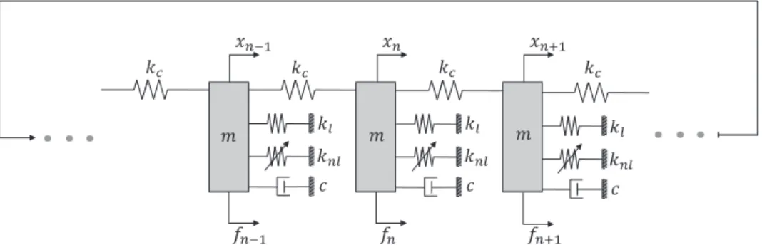
2. A lumped nonlinear model for cyclic symmetric structures The model under study consists of Ns identical oscillators with mass m,

cyclically connected to each other by linear springs kc, and also attached to

the ground by linear springs and viscous dampers kland c, respectively (Fig.

1). Each oscillator is also excited by an external force fn(t) and is subjected

to nonlinear forces induced by the cubic stiffness knl. The physical system

in Fig. 1 can be considered a minimal model for aerospace structures, e.g. blisks, antennas, or reflectors, undergoing large deformations.

݉ ݇௡௟ ݇௟ ܿ ݇௡௟ ݇௟ ܿ ݇௡௟ ݇௟ ܿ ݇௖ ݇௖ ݇௖ ݇௖ ݂௡ିଵ ݂௡ ݂௡ାଵ ݔ௡ିଵ ݔ௡ ݔ௡ାଵ ݉ ݉

Fig. 1 - Minimal model for a cyclic and symmetric structure undergoing large displacements

The equation of motion for the n-th oscillator is written as

m¨xn+ c ˙xn+ klxn− kc(xn+1+ xn−1− 2xn) + knlx3n= fn(t) (1)

where ¨xn, ˙xn, and xn are the acceleration, velocity, and displacement,

respec-tively, while fn(t) represents the corresponding external force applied to the

n-th mass. Equation (1) is rewritten, for convenience, such that ¨ xn+ 2ξω0˙xn+ ω₀2xn− ωc2(xn+1+ xn−1− 2xn) + γx3n = fn(t) m , (2) where ω2 0=k l m, ω 2 c= kc m, γ= knl m , and ξ= c

2√mkl. Finally, the set of nonlinear

differential equations is expressed in non-dimensional form as ¨

un+ 2ξ ˙un+ un− α(un+1+ un−1− 2un) + u3n = gn(τ ), (3)

where the dots represent the derivative with respect to the new time scale τ = ω0t, α = ω 2 c ω2 0, A = ω0 √γ, gn(τ ) = fn(t)

klA, and xn(t)=Au(τ ). Moreover, one

has the cyclic boundary condition uNs+1 = u1 and u0 = un.

3. Conservative regime: linear analysis

The linear and conservative regime of Eq. (3), for which the equation of motion is given by:

¨

has been previously studied in the literature (see e.g. Refs. [22]). The system has analytical travelling wave solutions such that

un(τ ) = Unkexp{i [k(n − 1)a − ωkτ ]} + c.c, (5)

where Uk _{is the complex wave amplitude, a = 2π/N}

s is the sector angle, k is

the wave number, ωk is the natural angular frequency, while c.c. states the

complex-conjugate of the first expression. After inserting Eq. (5) into Eq. (4), it is possible to demonstrate that the linear dispersion relation is given by

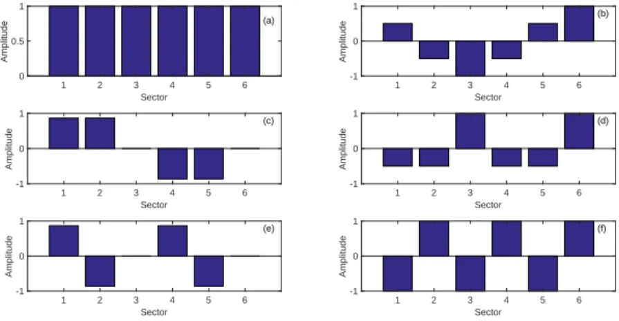
ω2_k= 1 + 2α [1 − cos(ka)] , (6) which represents the natural angular frequencies of Eq. (4). Moreover, the corresponding eigenvectors are obtained by substituting Eq. (6) into Eq. (5), and three different solutions are possible: (1) if k = 0 all masses move in phase such as Uk=0

n = 1; (2) if Ns is even k ∈ [1,N₂s − 1] (if Ns is odd k ∈

[1,(Ns₋₁₎

2 − 1]) two sets of solutions are possible such as U k,cos

n =cos((n − 1)ka)

and Uk,sin

n =sin((n − 1)ka); while (3) if k = N

s

2 the masses move out of phase

such as Uk=

n 2

n =(−1)n. In Fig. 2 the linear mode shapes are shown assuming

Ns = 6. Notice that the mode shapes (eigenvectors) do not depend on the

coupling parameter α. (a) 1 2 3 4 5 6 Sector 0 0.5 1 Amplitude (b) 1 2 3 4 5 6 Sector -1 0 1 Amplitude (c) 1 2 3 4 5 6 Sector -1 0 1 Amplitude (d) 1 2 3 4 5 6 Sector -1 0 1 Amplitude (e) 1 2 3 4 5 6 Sector -1 0 1 Amplitude (f) 1 2 3 4 5 6 Sector -1 0 1 Amplitude

4. Nonlinear normal modes

4.1. General analysis

In the nonlinear and conservative regime our investigation is based on the concept of nonlinear modes ([32],[33]). Therefore, periodic vibrations in the form of

¨

un+ un− α(un+1+ un−1− 2un) + u3n= 0 (7)

are computed using only one harmonic such as

un = Unexp{ωτ } + c.c., (8)

where Un is the complex-valued amplitude and ω is the nonlinear natural

angular frequency. The previous expression (8) is inserted into Eq. (7) and the resulting equation is projected into the Fourier basis which, neglecting higher order harmonics, leads to the following set of algebraic equations

(1 + 2α − ω2)Un+ 3Un3− α(Un+1+ Un−1) = 0. (9)

The solutions of Eq. (9) define the nonlinear normal modes (NNMs) of the physical system depicted in Fig. 1. Moreover, due to the amplitude de-pendency of the natural angular frequencies, some of the nonlinear mode shapes loose their homogeneity. Some modes can localize when the ampli-tude increases, i.e. only a small subset of the oscillators are vibrating with significant amplitudes.

The computation of the non-linear modes is carried out by solving Eq.(9) using a continuation procedure. In this study we used the numeric asymptotic method presented in ([34],[35]), and implemented in the MANLAB package. It is common to assume at low amplitude the initial points of the continuation procedure are given by the linear mode shapes, whereas other possible start-ing points at high amplitude will be described later. The results of the con-tinuation procedure provides the evolution of the natural angular frequency with respect to the amplitude of motion. One also obtains the evolution of mode shapes as the amplitude of vibration increases ([32],[33]). From the results, one can see that some mode shapes are similar (i.e. the shape does not depend on the amplitude of motion), and some others are non-similar. Potential bifurcation points of a given non-linear mode are computed search-ing for points where the determinant of the Jacobian matrix vanishes. The

Jacobian matrix of Eq. (9) is given by J =         ξ1 −α 0 . . . 0 −α −α ξ2 −α 0 . . . 0 . . . 0 . . . 0 −α ξ_{N −1} −α −α 0 . . . 0 −α ξN         (10)

with ξn = 1 + 2α − ω2+ 9Un2. At high amplitude the nonlinear term will be

dominant, hence the linear coupling between the oscillators can be neglected, therefore the system is equivalent to a series of uncoupled Duffing oscillators (for n ∈ [1, N]):

¨

un+ un+ u3n = 0 (11)

The eigen-shapes of such a system are given by the vectors of the canonical basis of RN_{, and the evolution of the angular frequency (for oscillator n) using}

a single harmonic HBM is given by ω2

n = 1 + 3Un2.

In the case of a non-linear modes motion, all (uncoupled) oscillators must have the same frequency, this is possible only if the amplitude are the same for all oscillators (Un = U0 or Un = −U0) or if some amplitudes are zero.

Therefore, at high amplitude, one expects that the mode shape will have the following general form:

φn= un, with un∈ {−1, 0, 1} (12)

In other words, there are three choices for each component of the mode shape. This leads to 3Ns different mode shapes at high amplitude. Those

mode shapes can be used as starting points for relatively high amplitude of motion to initiate the continuation procedure, which is carried out backward, i.e. in the direction of decreasing frequency. However, due to the symmetry of the system, several of those shapes belong to the same ”family”, i.e. they differ only by a rotation or by a change of sign (see Appendix - A). Without loss of generality, in the following we will choose only one representative for each ”family” to drastically decrease the number of possible initial points.

4.2. Nonlinear normal modes analysis for the present system

We start our investigation focusing on periodic solutions from the un-damped and unforced nonlinear system (9) assuming Ns = 6 and α = 0.01.

Therefore, the strategy proposed in Sub. 4.1 is employed to compute the NNMs of the underling conservative regime. The details of the derivation are not reported, while the main results are highlighted here:

• the first NNM Uk=0

n , when all masses vibrate in phase, is similar (its

shape does not change with amplitude) and does not bifurcate; • the NNM Uk=1,cos

n is non-similar and bifurcate twice;

• the NNM starting from Uk=1,sin

n is similar and does not bifurcate;

• the NNM starting from Uk=2,cos

n is similar and does not bifurcate;

• the NNM starting from Uk=2,sin

n is non-similar and bifurcates twice;

• the last NNM Uk=3

n , when all masses vibrate out of phase, is similar

and bifurcates eleven times.

Starting from the linear mode, and following the bifurcations, 22 classes of solutions have been computed (thin solid lines in Fig. 3). From symmetry consideration the number of possible solutions can be reduced from 3Ns = 729

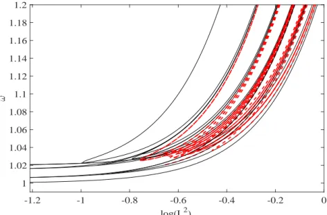
to 52 (including the trivial solution, see Appendix - A) 22 of which have been computed continuing the linear modes. In order to compute the remaining 30 modes, we use the corresponding shapes as a starting point at high amplitude for the continuation algorithm, and we start the continuation ”backward” (i.e. in the direction of decreasing frequency). This allows to compute new branches of solution in the Frequency Energy Plot (FEP) diagram (Fig. 3), where the L2 _{norm is defined as}

L2 = v u u t Ns X i=1 U2 n, (13)

The non-linear modes corresponding to those new branches are not con-nected to the other modes through bifurcation and appear as isolated branches on the FEP diagram (dashed thick red lines in Fig. 3). Those modes do no exist at low amplitude, but appear only after the energy is greater than a given threshold (depending on the mode). At high energy the nonlinear term is dominant and the oscillators behave as isolated. In fact the correspond-ing NNMs cluster into 6 groups, which energy depends on the number of oscillators vibrating with no negligible amplitude.

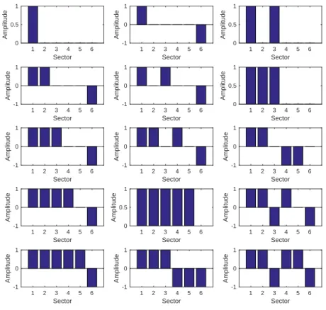
Fig. 4 reports some NNMs shapes (we have selected 15 out of the 52 solutions). Notice that possible solutions involve high localized ones with very few oscillators vibrating with appreciable amplitude.

-1.2 -1 -0.8 -0.6 -0.4 -0.2 0 log(L2) 1 1.02 1.04 1.06 1.08 1.1 1.12 1.14 1.16 1.18 1.2

Fig. 3 - FEP diagram of the nonlinear modes with their bifurcation. Thin solid black lines represent the solution of (9) starting, at low energy, from

the linear modes. Thick dashed red lines represent the solution of (9) starting at high energy and continuing them towards lower frequency (see

1 2 3 4 5 6 Sector 0 0.5 1 Amplitude 1 2 3 4 5 6 Sector -1 0 1 Amplitude 1 2 3 4 5 6 Sector 0 0.5 1 Amplitude 1 2 3 4 5 6 Sector -1 0 1 Amplitude 1 2 3 4 5 6 Sector -1 0 1 Amplitude 1 2 3 4 5 6 Sector 0 0.5 1 Amplitude 1 2 3 4 5 6 Sector -1 0 1 Amplitude 1 2 3 4 5 6 Sector -1 0 1 Amplitude 1 2 3 4 5 6 Sector -1 0 1 Amplitude 1 2 3 4 5 6 Sector -1 0 1 Amplitude 1 2 3 4 5 6 Sector 0 0.5 1 Amplitude 1 2 3 4 5 6 Sector -1 0 1 Amplitude 1 2 3 4 5 6 Sector -1 0 1 Amplitude 1 2 3 4 5 6 Sector -1 0 1 Amplitude 1 2 3 4 5 6 Sector -1 0 1 Amplitude

Fig. 4 - A selection of 15 (out of 52) nonlinear normal mode shapes with different degree of localization

5. Nonlinear forced and damped regime

5.1. Solution approach

In the present analysis we investigate the system described by Eq. (3) subjected to an external force

gn(τ ) = ˜Gnexp{iωFτ } + c.c., (14)

where ωF is the external force angular frequency and ˜Gn is the force

ampli-tude. To find the steady state periodic solutions of the system we adopt the harmonic balance method. Assume that, in the weakly nonlinear regime, the response un(τ ) is well approximated by a single harmonic such as

where ˜Un is a constant amplitude. After inserting Eqs. (14) and (15) into

Eq. (3) and projecting onto the truncated Fourier basis, the following set of nonlinear algebraic equations is obtained

(−ωF2 + 2iξωF + 1 + 2α) ˜Un− α( ˜Un+1+ ˜Un−1) + 3| ˜Un|2U˜n= Gn (16)

is obtained. Therefore, the amplitudes and phases of un(τ ) are defined by

the solutions of the algebraic system in Eq. (16).

5.2. Nonlinear forced responses

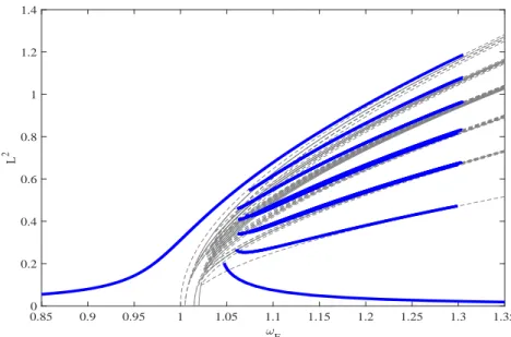
In this subsection we simulate the system in Fig. 1, as described by the non-dimensional form in Eq. (3), assuming Ns = 6 masses, ξ = 0.005

and weak coupling condition α = 0.01. A harmonic force is applied to each oscillator assuming a constant amplitude and phase value, such as

g(τ ) = G0exp{iωFτ } + c.c., (17)

where G0 is the force amplitude. One should note that the excitation is

perfectly orthogonal to all linear normal modes, except the first one which represents vibrations with all masses moving in phase. However, due to the presence of damping, the responses may vibrate with different phase values. For this purpose we used the continuation package AUTO, using as initial conditions highly loacalized guess for the vibration shape (e.g. [0,1,0,0,-1,0]) The system frequency response function (L2_{-norm vs angular frequency}

0.85 0.9 0.95 1 1.05 1.1 1.15 1.2 1.25 1.3 1.35 F 0 0.2 0.4 0.6 0.8 1 1.2 L 2 Unstable Stable

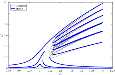
Fig. 5 - Frequency response function obtained for the chain of weakly coupled Duffing oscillators computed for three different force levels

G0 = [0.32, 1.3, 6.3] × 10−3

The results were computed using three different force levels, while blue thick lines indicate linearly stable solutions. The first response, computed for G0 = 3.2×10−4, illustrates the response when the nonlinear force is

negli-gible. The response is linear and single-valued. The second curve, computed for G0 = 1.3 × 10−3, shows already the stiffening effect induced by the cubic

stiffness. However, the responses are still homogeneous and no localization is observed. In the last case, when G0 = 6.3 × 10−3, the response shows

several bifurcated branches. The forced response shows multiple solutions within the frequency interval where the forced single oscillators exhibit two stable solutions for a given exciting frequency. Hence the forced response of the whole system is multivalued with many intertwining branches. The new branches seem to organize themselves similarly to snaking bifurcations ([36–38],[29]). In fact they fold alternating each individual oscillator from an upper branch to a lower one. Therefore, it is possible to observe solutions varying from states where energy is localized in just one oscillator, to solu-tions when energy is equally spread along the structure. This pattern is not much affected by the particular choice of cyclic (which we are using here) or free-free boundary conditions. Notice that, although the branches seem to

be all connected, in fact they aren’t, but appear as isolas of solutions, which get superposed in a two dimensional representation.

In order to provide a closer look at the transition from homogeneous states to localized ones, eq. (3) is solved for four different excitation levels. The results are depicted in Fig. 6 increasing the exciting force from panel (a) to panel (d) respectively. On the left column the frequency response function is reported, while, on the right column, the modulus of the vibration amplitude is shown for the labeled solutions. Linearly stable solutions are drawn with thick blue lines, unstable solutions with thin gray lines. Results in panel (a) have been computed for G0 = 1.6 × 10−3. It is shown that for low excitation

the response is quite homogeneous (Fig. 6, panel (a), right column) and only the unstable solution labeled with ”P4” shows some degree of localization. When the force is slightly increased to G0 = 2.4 × 10−3 (Panel (b)) other

branches of solutions are identified. Moreover, spatially localized linearly stable states appear. The bifurcation picture is mainly composed of two localized states detaching from the homogeneous solutions (P1 and P2), and two isolas that do not bifurcate from the main solution (solutions P3 and P4). Panel (c) and (d) are computed for G0 = 3.2 × 10−3 and G0 = 6.4 ×

10−3 _{respectively. It is shown that increasing the external excitation more}

branches are identified, and the isolas seem to evolve towards a final states where they merge with the upper branch of localized solution. Finally the final ”snaking bifurcation pattern” appears where the vibration gets localized from one single oscillator to the final homogeneous configuration either in the upper or in the lower branches. Comparing Fig. 4 and Fig. 6 one also notice the similarities between the NNM and forced responses shapes. Indeed, this behavior should be expected, as it is well known that the NNMs are the ”backbone curves” of the forced response and, at the resonance point, the forced system behaves alike the underlying NNM.

0.95 1 1.05 F 0 0.05 0.1 0.15 0.2 0.25 0.3 0.35 0.4 L 2 P1 P2 P3 P4 (a) P1 0 0.1 0.2 |x i | P2 0 0.1 0.2 |x i | P3 0 0.1 0.2 |x i | P4 1 2 3 4 5 6 Sector number 0 0.1 0.2 |x i | 0.95 1 1.05 1.1 F 0 0.1 0.2 0.3 0.4 0.5 L 2 P1 P2 P3 P4 (b) P1 0 0.1 0.2 |x i | P2 0 0.1 0.2 |x i | P3 0 0.1 0.2 |x i | P4 1 2 3 4 5 6 Sector number 0 0.1 0.2 |x i | 0.95 1 1.05 1.1 F 0 0.1 0.2 0.3 0.4 0.5 L 2 P1 P2 P3 P4 P5 (c) P1 0 0.2 |x i | P2 0 0.2 |x i | P3 0 0.2 |xi | P4 0 0.2 |x i | P5 1 2 3 4 5 6 Sector number 0 0.2 |x i | 1 1.1 1.2 1.3 F 0 0.2 0.4 0.6 0.8 1 1.2 L 2 P1 P2 P3 P4 P5 (d) P1 0 0.5 |x i | P2 0 0.5 |x i | P3 0 0.5 |xi | P4 0 0.5 |x i | P5 1 2 3 4 5 6 Sector number 0 0.5 |x i |

Fig. 6 - Form panel (a) to panel (d) the excitation force is G0 = [1.6, 2.4, 3.2, 6.4] × 10−3 respectively. For each panel on the left

column: frequency response function (blue thick lines for linearly stable solutions, thin gray lines for unstable solutions). For each panel on the

right column: vibration amplitude (in modulus) for each sector In Fig. 7 the nonlinear normal modes of the dynamical system (thin dashed lines) are superposed on the forced response (only stable solutions are reported with thick solid lines) for G0 = 6.3 × 10−3. It is clearly shown that

the local resonances of the mechanical systems are associated to a particular backbone curve. At high energy the response clearly clusters into 6 groups which correspond to the number of oscillators involved in the vibration.

0.85 0.9 0.95 1 1.05 1.1 1.15 1.2 1.25 1.3 1.35 F 0 0.2 0.4 0.6 0.8 1 1.2 1.4 L 2

Fig. 7 - The frequency response function of the mechanical system for G0 = 6.3 × 10−3 is superposed to the NNMs. Only the stable solutions of

the forced response are reported, while dashed lines represent the NNMs. 6. Conclusions

In this paper, the problem of vibration localization in externally excited weakly-coupled cyclic symmetric structures affected by geometrical nonlin-earities has been considered. The model we have set-up is constituted by a cyclic symmetric chain of six Duffing oscillators, where stiffening effects have been considered via a cubic stiffness term. The nonlinear normal modes have been computed. Due to symmetry considerations, the system periodic solu-tions can be classified into 52 different shapes (including the trivial one). It has been shown that 22 of them are obtained starting from the linear modes and following their bifurcation from low to high amplitude. The remaining 30 solutions, instead, appear to be isolated branches, detached from the other modes. The isolated branches exist only after a certain energy threshold is reached and disappear at low energy.

When the cyclic symmetric chain is forced with the first linear mode shape (all the oscillators are excited with the same force) spatial localized vibrating states appear. The degree of localization is strongly dependent on the excitation strength. For strong excitation more localized branches

appear, which, in the bifurcation diagram arrange similarly to snaking bi-furcations. When the backbone curves of the nonlinear normal modes are superposed with the forced response they appear to match almost exactly, showing that the intermediate states between the low and high energy states correspond to local resonances of the system. We have shown that this be-haviour is strongly related to the bistable bebe-haviour of the single nonlinear oscillators from which the chain is formed: if the excitation level is low, the bistable range disappears, the system behaves nearly linearly and there is no localization. In the latter case, there is no localization.

The results of the present study may be of interest for aerospace/aeronautical applications, where the quest of high performance is leading to lightweight and slender structures, often characterized by weak nearest neighbor coupling (e.g. fan blades or antennas). Due to high flexibility, the latter are prone to large oscillations thus to nonlinear stiffening effects. This work shows that vibration localization in space can arise due to nonlinear phenomena, which represents a different mechanism with respect to mistuning. Further studies are needed to better understand how the presently demonstrated nonlinearly triggered localization effect interacts with linear localization phenomena such us mistuning.

Author Contribution Statement

AP and FF conceived the work. FF computed the numerical results. AG did the NNM analysis. AP wrote the paper and coordinated all the work. MC and NH supervised the work.

Acknowledgements

AP is thankful to the DFG (German Research Foundation) for funding the projects PA 3303/1-1 and HO 3852/11-1.

Appendix A: sorting initial points using symmetry

Denote E the set of all possible initial points at high amplitude. There are |E| =card(E) = 3Ns

possible choices, i.e. 3 choices [1, 0, −1] for the Ns

components.

In order to reduce the number of initial points, one can use the fact that the algebraic system defining the non-linear modes in Eq. (9) is equivariant under several groups:

• The cyclic group CN, which representation in a N dimensional space is

generated by the N × N matrix R given by the following:

R=            0 1 0 0 0 0 0 0 1 0 0 0 ... . .. ... 0 0 0 0 1 0 0 0 0 0 0 1 1 0 0 0 0 0            (18)

• The axial symmetry, generated by the N × N matrix S given as:

S=            1 0 0 0 0 0 0 0 0 0 0 1 0 0 0 0 1 0 ... ... ... 0 0 1 0 0 0 0 1 0 0 0 0            (19)

• The ”sign-change” symmetry (related to the fact that we are looking for ”symmetric” periodic solution such that u(t + T

2) = −u(t)), generated

by the N × N matrix C given as:

C=          −1 0 0 0 0 0 −1 0 0 0 ... . .. ... 0 0 0 −1 0 0 0 0 0 −1          (20)

To sum up the algebraic system is equivariant under a group G, having |G| = 4N elements, which can be represented as:

G = {gijk = SiCjRk, with (i, j, k) ∈ [0, 1] × [0, 1] × [0, N − 1]} (21)

For the case Ns= 6 taking into account the symmetry conditions, the number

of initial points reduces from |E| = 3Ns

= 729 to only 52, which includes the trivial one with all 0.

References References

[1] R. Bartels, A. Sayma, Computational aeroelastic modelling of airframes and turbomachinery: progress and challenges, Philos. Trans. R. Soc. A 365 (1859) (2007) 2469e2499, https://doi.org/10.1098/rsta.2007.2018 [2] D. J. Ewins, The effects of detuning upon the forced vibrations of bladed

disks. Journal of Sound and Vibration, 9(1) (1969) 65IN273-7279. [3] A. Martin, F. Thouverez, Dynamic Analysis and Reduction of a Cyclic

Symmetric System Subjected to Geometric Nonlinearities. ASME. Turbo Expo: Power for Land, Sea, and Air, Volume 7C: Structures and Dynamics ():V07CT35A015. doi:10.1115/GT2018-75709.

[4] O.O. Bendiksen, Mode localization phenomena in large space structures, AIAA Journal, Vol. 25, No. 9 (1987), pp. 1241-1248.

[5] A. J. Dick, B. Balachandran, & C. D. Mote, Intrinsic localized modes in microresonator arrays and their relationship to nonlinear vibration modes, Nonlinear Dynamics, 54.1-2, (2008), 13-29.

[6] A. J. Dick, B. Balachandran, & C.D. Mote, Localization in microres-onator arrays: influence of natural frequency tuning. Journal of Com-putational and Nonlinear Dynamics, 5(1), (2010), 011002.

[7] C. H. Hodges, Confinement of vibration by structural irregularity. Jour-nal of sound and vibration, 82(3) (1982) 411-424.

[8] D. S. Whitehead, (1966). Effect of mistuning on the vibration of turbo-machine blades induced by wakes. Journal of Mechanical Engineering Science, 8(1), 15-21.

[9] M.P. Castanier, P. Christophe, Modeling and analysis of mistuned bladed disk vibration: current status and emerging directions. Journal of Propulsion and Power 2 (2006) 384-396

[10] P.W. Anderson, Absence of diffusion in certain random lattices, Phys. Rev., 109(5) (1958) 1492-1505.

[11] K.Y. Sanliturk, D. J. Ewins, A. B. Stanbridge. Underplatform dampers for turbine blades: theoretical modelling, analysis and comparison with experimental data. ASME 1999 international gas turbine and aeroengine congress and exhibition. American Society of Mechanical Engineers, 1999.

[12] C. M. Firrone, S. Zucca,. Underplatform dampers for turbine blades: The effect of damper static balance on the blade dynamics. Mechanics Research Communications, 36(4) (2009) 515-522.

[13] A. Papangelo, M. Ciavarella, On the limits of quasi-static analysis for a simple Coulomb frictional oscillator in response to harmonic loads. Journal of Sound and Vibration, 339, (2015) 280-289.

[14] A. Papangelo, M. Ciavarella. Optimal normal load variation in wedge-shaped Coulomb dampers. The Journal of Strain Analysis for Engineer-ing Design, 51(4), (2016) 279-285.

[15] L. Pesaresi, L. Salles, A. Jones, J.S. Green, C.W. Schwingshackl. Mod-elling the nonlinear behaviour of an underplatform damper test rig for turbine applications. Mechanical Systems and Signal Processing, 85, (2017) 662-679.

[16] L. Pesaresi, L. Salles, R. Elliott, A. Jones, J. S. Green, C. W. Schwing-shackl. Numerical and experimental investigation of an underplatform damper test rig. In Applied Mechanics and Materials (849), (2016) 1-12 [17] A.F. Vakakis, L.I. Manevitch, Y.V. Mikhlin, V.N. Pilipchuk, A.A. Zevin, Normal Modes and Localization in Nonlinear Systems, John Wiley & Sons Inc, New York, 1996.

[18] G. Kerschen, M. Peeters, J.C. Golinval, A.F. Vakakis, Nonlin-ear normal modes, Part I: a useful framework for the structural dynamicist, Mech. Syst. Signal Process. 23 (1) (2009) 170e194, https://doi.org/10.1016/j.ymssp.2008.04.002.

[19] A. Papangelo, A. Grolet, L. Salles, N. Hoffmann, M. Ciavarella, Snaking bifurcations in a self-excited oscillator chain with cyclic symmetry. Com-munications in Nonlinear Science and Numerical Simulation, 44 (2017a) 108-119.

[20] A. Papangelo, M. Ciavarella, N. Hoffmann, Subcritical bifurcation in a self-excited single-degree-of-freedom system with velocity weakening-strengthening friction law: analytical results and comparison with ex-periments. Nonlinear Dynamics, 90(3) (2017b) 2037-2046.

[21] A. Papangelo, N. Hoffmann, A. Grolet, M. Stender, M. Ciavarella, M., Multiple spatially localized dynamical states in friction-excited oscillator chains. Journal of Sound and Vibration, 417 (2018) 56-64.

[22] A. Grolet, F. Thouverez, Free and forced vibration analysis of a non-linear system with cyclic symmetry: Application to a simplified model. Journal of sound and vibration, 331(12) (2012) 2911-2928.

[23] F. Fontanela, A. Grolet, L. Salles, A. Chabchoub, N. Hoffmann, Dark solitons, modulation instability and breathers in a chain of weakly non-linear oscillators with cyclic symmetry, Journal of Sound and Vibration, 413 (2018) 467-481.

[24] Y. Starosvetsky, L.I. Manevitch, On intense energy exchange and local-ization in periodic FPU dimer chains, Phys. D: Nonlinear Phenom. 264 (2013) 66-79, https://doi.org/10.1016/j.physd.2013.06.012.

[25] M.P. Castanier, C. Pierre, Using intentional mistuning in the de-sign of turbomachinery rotors, AIAA J. 40 (10) (2002) 2077e2086, https://doi.org/10.2514/3.15298.

[26] F. Georgiades, M. Peeters, G. Kerschen, J.C. Golinval, M. Ruzzene, Modal analysis of a nonlinear periodic structure with cyclic symmetry, AIAA J. 47 (4)(2009) 1014e1025, https://doi.org/10.2514/1.40461. [27] O.O. Bendiksen, Mode localization phenomena in large space structures,

AIAA J. 25 (9) (1987) 1241e1248, https://doi.org/10.2514/3.9773. [28] O.O. Bendiksen, P.J. Cornwell, Localization of vibrations

in large space reflectors, AIAA J. 27 (2) (1989) 219e226, https://doi.org/10.2514/3.10084.

[29] A.R. Champneys, Homoclinic orbits in reversible systems and their ap-plications in mechanics, fluids and optics. Physica D: Nonlinear Phe-nomena, 112.1 (1998) 158-186.

[30] O. Thual , and S. Fauve, Localized structures generated by subcritical instabilities. Journal de Physique 49.11 (1988) 1829-1833.

[31] C. Beaume, A. Bergeon, E. Knobloch, Homoclinic snaking of localized states in doubly diffusive convection. Physics of Fluids, 23(9) (2011) 094102.

[32] R. M. Rosenberg, The normal modes of nonlinear n-degree-of-freedom systems. Journal of applied Mechanics, 29(1) (1962) 7-14.

[33] S. W. Shaw, C. Pierre, Normal modes for non-linear vibratory systems. Journal of sound and vibration, 164(1) (1993) 85-124.

[34] B. Cochelin, N. Damil and M. Potier-Ferry. ” Asymptotic-Numerical Methods and Pad´e approximants for non- linear elastic structures” Int. J. Numer. Methods Engng , Vol 37, p 1187-1213, 1994.

[35] B. Cochelin. ” A path following technique via an Asymptotic-Numerical method” Computers & Structures, Vol 53, N◦ _{5, p 1181-1192, 1994.}

[36] Hunt, G. W., Lord, G. J., A.R. Champneys, Homoclinic and hetero-clinic orbits underlying the post-buckling of axially-compressed cylin-drical shells. Computer methods in applied mechanics and engineering, 170(3-4) (1999) 239-251.

[37] G.W. Hunt, M.A. Peletier, A.R. Champneys, P.D. Woods, M. A. Wadee, C.J. Budd, G.J. Lord, Cellular buckling in long structures. Nonlinear Dynamics, 21(1) (2000) 3-29.

[38] J. Burke, E. Knobloch, Homoclinic snaking: structure and stability. Chaos: An Interdisciplinary Journal of Nonlinear Science, 17(3) (2007) 037102.