Science Arts & Métiers (SAM)
is an open access repository that collects the work of Arts et Métiers Institute of Technology researchers and makes it freely available over the web where possible.
This is an author-deposited version published in: https://sam.ensam.eu Handle ID: .http://hdl.handle.net/10985/12794
To cite this version :
Etienne BALMES, Guillaume VERMOT DES ROCHES, Thierry CHANCELIER, Guillaume MARTIN - Squeal measurement using operational deflection shape. Quality assessment and analysis improvement using FEM expansion. - In: Eurobrake, Allemagne, 2017-05 - Proceedings Eurobrake - 2017
Any correspondence concerning this service should be sent to the repository Administrator : [email protected]
EB2017-VDT-018
Squeal measurement using operational deflection shape. Quality assessment
and analysis improvement using FEM expansion.
1,3Martin, Guillaume*; 1,3Balmes, Etienne; 1Vermot-Des-Roches, Guillaume ; 2Chancelier, Thierry
1SDTools, France; 2Chassis Brakes International, France; 3Arts & Metiers ParisTech, PIMM, France
KEYWORDS – Operational Deflection Shapes, limit cycle, shape expansion
ABSTRACT – In presence of squeal, Operational Deflection Shapes (ODS) are classically measured to gain understanding of brake behavior. A simple numeric example is analyzed to justify the use of time-frequency analysis and shows that two real shapes should probably dominate the response. Using measurements on a real brake, this expectation is shown to hold even in the presence of variations with wheel position as well as for reproducibility tests. For a proper relation with the model, it is desirable to also extract modes. The test campaign is used to illustrate how this can be quite difficult due to reproducibility problems. Finally, shapes characterizing the squeal event are fundamentally limited by measurable quantities. Minimum Dynamic Residual Expansion (MDRE), which estimates test motion at all FE degrees of freedom, is shown to be applicable for industrial models and gives insight of test and model imperfections.
INTRODUCTION
Squeal being an undesired condition, its appearance is never predicted by initial design models, when they exist, and experiments are needed to understand the exact conditions of occurrence. Models are however necessary to understand how measurements should be post-processed to obtain characteristic shapes that will later be used to propose design changes. Finite element models are also necessary to estimate unmeasured motion using expansion techniques that will be detailed here and evaluate the impact of modifications.
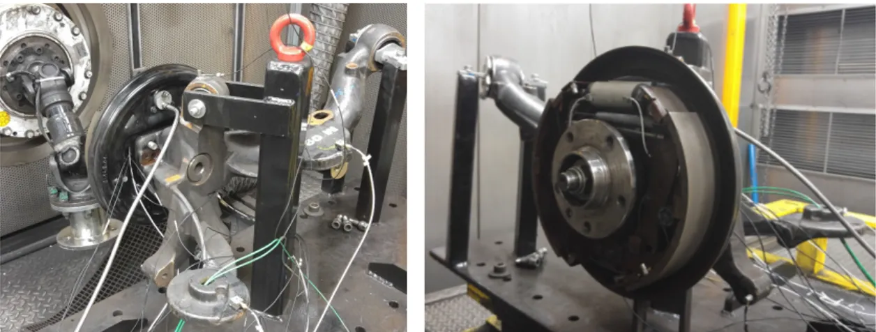
All measurements used throughout this paper have been performed on a drum brake system shown in Figure 1. On the pictures, the drum was removed to see the internal instrumentation. For this brake, a low frequency squeal occurrence (about 900Hz) has been found on vehicle and needed to be reproduced on bench for further analysis.
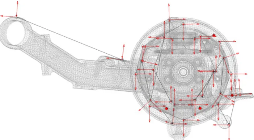
The measurement geometry has been built from the numerical mode shapes, using the MSeq algorithm [1], to distinguish the modes in a frequency band around 900Hz. The provided sensor placement was then adapted to the constraint of positioning feasibility and each sensor location was in finally measured using triax sensors to also permit the direct exploitation (at least visual) of the measurement without the use of expansion if needed : visual interpretation of shapes is very difficult with uniaxial sensors. The experimental wireframe geometry, on top of the FEM is shown in Figure 2
Figure 2 : Measurement wireframe on top of the FEM
Due to the high number of sensors and the limited number of measurement channels, 4 sequential measurement batches are needed and 4 uniaxial reference sensors will be used to control the merging quality.
The aim of the measurement campaign was to extract so called Operational Deflection Shapes (ODS) to characterize the limit cycle found during a squeal occurrence. The classic procedure at CBI is to generate a single spectrum associated with a squeal occurrence and extract a shape associated with a main resonance. The simple numerical model discussed in Section 1 illustrates that the shapes associated with squeal instabilities are expected to be dominated by the combination of two real modes but that the combination may be quite sensitive to changes.
Knowing that a limit cycle is expected to be composed of a time varying combination of two shapes, Section 2 exploits time-frequency analyses of the measurements to demonstrate that indeed two real shapes dominate the response and have variations that are coherent with the changes due wheel position. A reproducibility test further shows that, while different experiments can lead to notable frequency shifts, the shapes underlying the limit cycle are fairly constant.
Section 3 then illustrates that transfers measured to allow classical modal extraction show major shifts in reproducibility tests so that proper extraction of modeshapes appears as a challenge needing the development of novel methods.
Finally, the spatial resolution of the test remains quite low even if sequential measurement batches are merged. As a result, using modeshapes expansion techniques to estimate the full FE response from measurements appears as a necessity to provide understanding of
inconsistencies between model and test and thus pave the way for the proposition of
modifications. The Minimum Dynamic Residual (MDRE) method [2] is applied in Section 4 to illustrate the potential uses. It is shown that expanded shapes give better understanding of the brake motion and that repartition of the residual energy after expansion gives insight on modeling errors.
1. EXPECTED SHAPES IN A SQUEAL EVENT : A SIMPLE EXAMPLE
To motivate the procedure used to analyze shapes during a squeal event, a simple numeric example is analyzed here. Without going into the details, which can be found in [3], the complex mode shapes come from the linearization of the model around a chosen state (pressure, velocity…). The linearized model provides a system of the form
[𝑀]{𝑞̈(𝑡)} + [𝐶]{𝑞̇(𝑡)} + [𝐾 + 𝐾 ]{𝑞(𝑡)} = {𝑓 (𝑡)} (1) where 𝑞, 𝑞̇ et 𝑞̈ are displacements, velocities and acceleration, M, C, K are respectively the mass, damping and stiffness matrices supposed constant. The stiffness matrix can be decomposed in a symmetric part 𝐾 , coming from the elastic properties of each components and the linearization of the normal contact loads and a non-symmetric part 𝐾 linked to the fluctuation of the tangential loads induced by the fluctuation of the normal loads. It is classical to project the system in the so-called real mode basis [𝛷], found by solving the system with [𝐶] = 0 and 𝐾 = 0 (which is equivalent to consider a friction coefficient 𝜇 = 0). The system to solve is then
∖𝜔
\ + [𝛷 𝐾 𝛷] + 𝜆 [𝛷 𝐶𝛷] + 𝜆 [𝐼] 𝜓 = 0 (2)
with the spatial Degrees Of Freedom (DOFs) linked to the reduced ones by 𝜓 = [𝛷]{𝜓 }. The numeric case is a simplified brake of which the mesh geometry is shown in Figure 3. The disc (blue) and the backplate (yellow) materials is steel and the friction (green) is made of an orthotropic softer material, about 5GPa with an additional Rayleigh damping (see the
introduction of [3] for details). The model is clamped at 4 locations at the interface between the backplate and the friction (similar to the one circled in the figure).
Figure 3 : Simple brake model geometry (left) and real mode shapes #8 and #9. (right)
This model has an unstable (negative damping) complex mode at 5050Hz which corresponds to the interaction between the two real modes #8, with a mostly out-of-plane deformation, and #9 with mostly a deformation of the pads sliding on the disc.
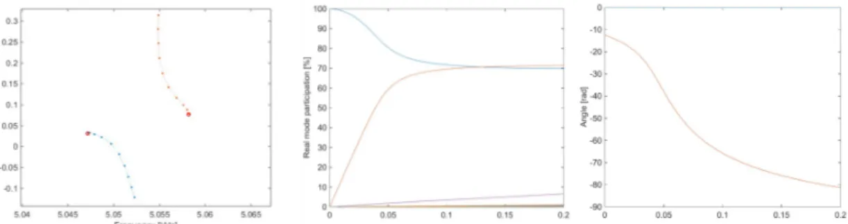
To confirm that the complex mode shape mainly comes from the interaction between the two real mod shapes, the friction coefficient is swept from 0 to 0.2 (not a physical value but still relevant for the interpretation). The left of Figure 4 shows that the two firstly stable (red circles) complex modes (#8 and #9) evolve with the increase of the friction coefficient. Mode #8 becomes unstable while the mode #9 is more and more damped.
Figure 4 : Evolution of complex modes with the friction coefficient: roots (left), real mode participation to the complex mode #8 (middle) and phase between real modes #8 and #9 (right)
From Equation 4, it is possible to look at the evolution of the real mode participation (𝜓 ) of each modal DOF with the normalization ‖𝜓 ‖ = 1. At the middle of Figure 4, the
participation of the real modes to the complex mode #8, which become unstable, evolves from 100% of real mode #8 (blue line) to 70% of real mode #9 (red line) and 70% of real mode #8. Dephasing also occurs: the left of Figure 4 shows the evolution of the phase between the real modes #8 and #9 in their contributions to the complex mode #8.
To evaluate the pertinence to use only two real modes to interpret the unstable modes, the Equation 4 is reduced on the 2 real mode shapes #8 and 9, leading (with the assumption of modal damping) to 1 0 0 1 𝜆 + 2𝜁 𝜔 0 0 2𝜁 𝜔 𝜆 + 𝜔 0 0 𝜔 + 𝑘 𝑘 𝑘 𝑘 𝜓 = 0 (3)
The comparison between the system reduced on the 2 real modes on the one hand and on all real modes on the other hand is provided by Figure 5. The precision on the complex mode frequencies is worst when considering two real modes for reduction, but the coupling still occurs and the damping computation is almost unchanged.
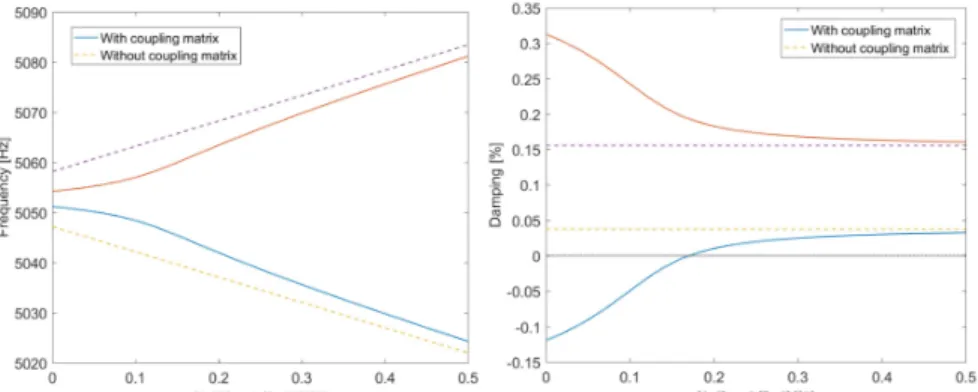
Figure 5 : Comparison between complex modes frequencies (left) and dampings (right) for reduction on 2 real modes (dashed lines) and on all real modes (full lines).
The common practice in presence of coupled modes is to try moving the frequencies away from each other. Doing so on the model reduced on two real mode shapes, by moving away their frequencies with the same percentage (modifying 𝑘 , 𝑘 , 𝑐 , 𝑐 but not the non-symmetric stiffness part), results in the evolution of the complex frequencies and damping shown in Figure 6. As mode #9 damping decreases, mode #9 one increases until it is no more unstable. The dot lines represent the values of the frequencies 𝑓 𝑓 and dampings 𝜁 𝜁 . When the frequencies are moved away, the influence of the coupling stiffness decreases and the mode parameters converge toward the ones without coupling at all.
Figure 6 : Evolution of the complex mode frequencies and dampings by moving away the frequencies of real modes #8 and #9
2. TIME FREQUENCY ANALYSIS
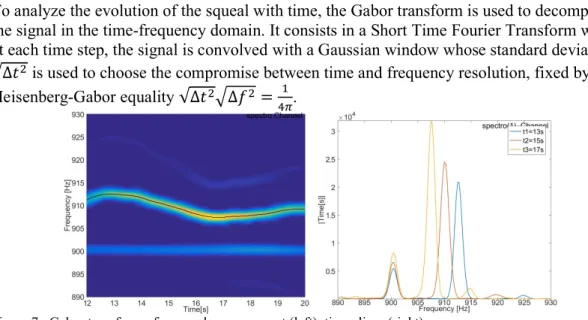
To analyze the evolution of the squeal with time, the Gabor transform is used to decompose the signal in the time-frequency domain. It consists in a Short Time Fourier Transform where at each time step, the signal is convolved with a Gaussian window whose standard deviation √∆𝑡 is used to choose the compromise between time and frequency resolution, fixed by the Heisenberg-Gabor equality √∆𝑡 ∆𝑓 = .
Figure 7 : Gabor transform of a squeal measurement (left), time slices (right)
The Gabor transform is applied to the measurement on an arbitrary sensor with a very good frequency resolution ∆𝑓 = 0.5𝐻𝑧 which induces a quite poor time resolution √∆𝑡 = 0.1592𝑠, acceptable because the squeal behavior evolution with time is slow. The Figure 7 left shows that during the squeal, the frequency shifts between 906Hz and 913Hz. Three time slices on the right of the figure also highlight the amplitude evolution of the main resonance. A smaller peak of amplitude, constant in frequency at 900Hz, is present for each measurement and is due to a harmonic of the power supply of the bench (50Hz).
To evaluate in detail the evolution of the behavior, at each instant 𝑡, the frequency where the amplitude is maximum 𝑓 (𝑡) is found, and the corresponding shape {𝑦(𝑓 (𝑡), 𝑡)} is extracted. All these shapes are concatenated and real plus imaginary parts are decomposed with the Singular Value Decomposition providing sorted real shapes 𝑈
[𝐹] = [ℜ(⋯𝑦(𝑓 (𝑡), 𝑡)⋯) ℑ(⋯𝑦(𝑓 (𝑡), 𝑡)⋯)] × = 𝑈 𝜎 𝑉 (4) with NS the number of sensors and NT the number of time steps.
The family [⋯𝑦(𝑓 (𝑡), 𝑡)⋯] can then be decomposed on these real shapes, leading to [⋯𝑦(𝑓 (𝑡), 𝑡)⋯] ≈ 𝑈
× 𝑎 (𝑡) × (5)
with 𝑎 (𝑡) = 𝜎 × (𝑣 (𝑡) + 𝑖𝑣 (𝑡 + 𝑁𝑇)).
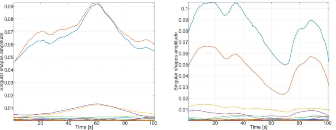
Figure 8 : Time evolution of the main real shapes 𝑎 (𝑡) (left) and relative evolution between the two main shapes 𝑎 (𝑡)/𝑎 (𝑡).
The Figure 8 shows on the left the time evolution of 𝑎 (𝑡) and it is clear that the limit cycle shapes rely only in a 2 dimension space engendered by the two main real shapes [𝑈 𝑈 ]. The relative evolution between the two main shapes 𝑎 (𝑡)/𝑎 (𝑡) is analysed in the right showing a quite high important evolution in amplitude in the range 0.75-1 and a low phase evolution between -85° and -100°. The variability of the limit cycle, despite the evolution of the complex shape, stays in the same subspace in an analogous way than the numerical result regarding the evolution of the unstable complex modes with the friction coefficient. The reproducibility needs then to be evaluated. For this purpose, a second squeal has been measured a day after the first measurement, leading to potential evolution of parameters such as pressure map, relative component placement or temperature. The time-frequency evolution of this second measurement and for the same sensor is shown on Figure 9. A quite important frequency shift is also found from 917Hz to 925Hz and is in average more than 10Hz higher than the first one.
Figure 9 : Gabor transform of the second squeal measurement.
The family containing the two measurement, normalized to have the same weight [𝑦(𝑡)] = [⋯𝑦 (𝑓 (𝑡), 𝑡)⋯]
‖⋯𝑦 (𝑓 (𝑡), 𝑡)⋯‖
[⋯𝑦 (𝑓 (𝑡), 𝑡)⋯]
‖⋯𝑦 (𝑓 (𝑡), 𝑡)⋯‖ (6)
is used and decomposed in the same way than previously with Equations 4 and 5. The evolutions of the amplitudes 𝑎, (𝑡) and 𝑎, (𝑡) , related to the common main real shapes shown in Figure 10. The predominance of the two main real shapes is a bit less clear than when the first measurement was decomposed alone (see Figure 8 left), but still there.
Figure 10 : Time evolution of the common main real shape amplitudes for the first measurement 𝑎, (𝑡) (left) and the second measurement 𝑎, (𝑡) (right).
Using the hypothesis that iterative squeal measurements rely on the same subspace, an algorithm to merge the 4 measurement batches using the 4 common sensors has been developed. It is not possible to enter into the details in this paper, but the result provides two real main shapes at all sensors which can then be exploited as a whole to analyze the
deformations or to perform expansion using a FEM. 3. TRANSFERS FOR MODAL EXTRACTION
In the previous section, the extracted shapes correspond to the limit cycle during the squeal, providing mainly two shapes. For model updating purpose, the classical way to tune the model parameters is to use experimental mode shapes as references. Many studies on the field of extracting modal data in operating conditions have been performed, and an interesting review can found in [4]. For this first test, a classical Experimental Modal Analysis has been implemented, using an electrodynamic shaker.
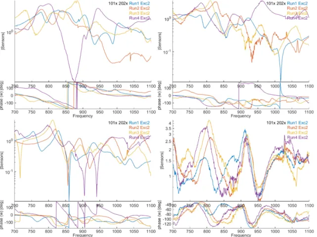
The exploitation of the mode shapes for correlation activities needs a good representability of the operating conditions and a good reproducibility. To evaluate the dependency to the operating conditions, several measurements were realized. From the least to the most representative operating conditions, we considered: braking under 20bars without sliding, then addition of 100Nm torque, then 200Nm torque and finally under sliding conditions. The repeatability is evaluated by comparing the transfers between a position of the shaker and an arbitrary reference sensor, measured for each of the 4 batches. The Figure 11 shows for each operating condition the superposition of the 4 transfers.
Figure 11 : Reproducibility of transfers for the position #2 of the shaker and the reference #1, under 20 bars for different operating conditions: static (top left), 100Nm torque (top right), 200Nm torque (bottom left) and under sliding conditions (bottom right).
The repeatability for the static measurement is very poor : the 4 transfers are very different. With the addition of the torque, especially with 200Nm, some similitudes between the transfers can be found, but the merging seems nevertheless at worst very difficult to put in place and at best with a very doubtful result quality. Moreover, the capability to make the link with the squeal which occurs in sliding condition remains a question.
With the sliding conditions, the noise level is higher than for the other transfers. This is due to the internal loads induced by the sliding between the drum and the shoes. Their effects on the response are considered uncorrelated to those engendered by the controlled input force and thus removed by the several averages (the H1 estimator is used). Despite the higher noise level, the repeatability is better with a resonance around 900Hz. The merging seems possible and the operating conditions are closer to the squeal ones.
Extraction and evaluation of the mode shapes from measurement under sliding conditions are a perspective. The need for a time-frequency identification algorithm, allowing taking into account the fluctuations during braking, is a question.
4. EXPANSION METHODS APPLIED TO THE TEST CASE
The two shapes obtained from the exploitation of the limit cycle measurements are used to perform expansion with a FEM. The MDRE [2] algorithm is used, which consist in finding the shape 𝜙 that minimize the weighted sum of two energies: 𝜖 linked to the residual force 𝑍(𝜔) 𝜙 = 𝑑𝐹(𝜔) (not zero because the model is not exact) and 𝜖 linked to the measurement error (the error between the measured shape and the observation at sensors of
𝜙 ). The cost function is then written
𝐽 = 𝜖 + 𝛾𝜖 with 𝛾 the ponderation between the two errors.
The FEM is reduced on a basis combining the response to unit loads at sensors, for the result to be at least as good as the static expansion, and the free modes of the structure, for the expansion to be exact if the model matches perfectly the measurements. This family of shapes is orthonormalized with respect to mass and stiffness matrices, leading to the basis
[𝑇] = [𝛷] [𝛷 ]
with [𝛷] the free mode shapes and [𝛷 ] the part of the response to unit loads at sensors that is orthogonal to the free modes (this part will be called later enrichment).
The interest of this model reduction is that it can be useful if the expansion is used in
combination with an updating procedure, to speed up the parametrized studies. It also permits a quick evaluation of the MDRE result with several values of the parameter 𝛾 which allows more or less measurement error.
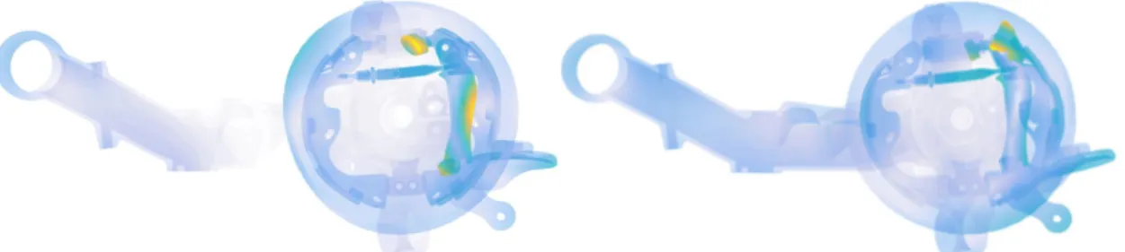
The expanded shapes are shown in Figure 12. The first one is dominated by the deformation of the brake lever. The second shape is mostly a deformation of the right shoe. The analysis of the squeal behavior with the expanded shapes is simpler than with only the deformations at sensors. It can help providing modification propositions to impact the phenomenon.
Figure 12 : Expansion result for the two extracted experimental shapes form the limit cycle measurements.
The expansion can also be used to analyze the model quality. Indeed, the repartition of the energy coming from the residual forces shows areas of the model where the mechanical equilibrium is poor. This residual energy can be split in two: the residual energy related to the free mode shapes, and the residual energy related to the enrichment shapes.
The Figure 13 shows the repartition of the residual energy related to the enrichment shapes: it is mostly a concentration of energy at the sensor locations. Those with the highest energy are on the brake lever (A), at the middle of the shoe (B) and at the attachment + the middle of the arm (C).
Figure 13 : Model error on the enrichment shapes
The Figure 14 shows the repartition of the residual energy on the free mode shapes. This energy is more global with nevertheless several concentration areas: in the arm (A),
confirming the need to look at the definition of the attachments to the ground and possibly to perform an updating of the component, close to the contact between the plate and the arm (B), and at two contacts between the shoe and the plate (C).
Figure 14 : Model error on the free mode shapes
A B C C C A B C C A
Using these residual energy maps helps in defining a relevant parametrization of the model to perform model updating if needed.
5. CONCLUSION
This study shows that the interpretation of the squeal behavior as an interaction between two real shapes makes sense, not only numerically but also experimentally. The reproducibility of the phenomenon, despite frequency shifts, is good when the subspace is compared instead of the complex shapes directly: the limit cycle lies in a two dimension subspace with a slow relative evolution.
The extraction of mode shapes needs measurements in sliding conditions to be closer to the squeal conditions and to gain in reproducibility of the measurements. The extraction of the modeshapes on the sliding conditions and possibly the use of an algorithm taking into account the presence of internal forces and the possibly time varying nature of the system is a
perspective.
Finally, the expansion of the two shapes extracted from the limit cycle measurements is useful to better interpret the brake behavior. It can moreover be used to find areas where the model seems wrong and thus to help in the definition of a relevant model updating study. The updating of this model and its impact on the expansion result is another perspective of this work.
REFERENCES
[1] E. Balmes and others, “Orthogonal Maximum Sequence Sensor Placements Algorithms for modal tests, expansion and visibility,” IMAC January, vol. 145, p. 146, 2005. [2] E. Balmes, “Review and Evaluation of Shape Expansion Methods,” Int. Modal Anal.
Conf., pp. 555–561, 2000.
[3] G. Vermot Des Roches, “Frequency and time simulation of squeal instabilities.
Application to the design of industrial automotive brakes,” Ecole Centrale Paris, CIFRE SDTools, 2010.
[4] E. Reynders, “System identification methods for (operational) modal analysis: review and comparison,” Arch. Comput. Methods Eng., vol. 19, no. 1, pp. 51–124, 2012.