Université de Montréal
Traffic Prediction and Bilevel Network Design
par
Léonard Ryo Morin
Département d’informatique et de recherche opérationnelle Faculté des arts et des sciences
Thèse présentée en vue de l’obtention du grade de Philosophiæ Doctor (Ph.D.)
en Informatique
10 janvier 2020
c
Université de Montréal
Faculté des études supérieures et postdoctoralesCette thèse intitulée
Traffic Prediction and Bilevel Network Design
présentée par
Léonard Ryo Morin
a été évaluée par un jury composé des personnes suivantes :
Jean-Yves Potvin (président-rapporteur) Emma Frejinger (directrice de recherche) Bernard Gendron (codirecteur) Fabian Bastin (codirecteur) Margarida Carvalho (membre du jury) Carolina Osorio (examinatrice externe) Jacques Bélair
Résumé
Cette thèse porte sur la modélisation du trafic dans les réseaux routiers et comment celle-ci est intégrée dans des modèles d’optimisation. Ces deux sujets ont évolué de manière plutôt disjointe: le trafic est prédit par des modèles mathématiques de plus en plus complexes, mais ce progrès n’a pas été incorporé dans les modèles de design de réseau dans lesquels les usagers de la route jouent un rôle crucial. Le but de cet ouvrage est d’intégrer des modèles d’utilités aléatoires calibrés avec de vraies données dans certains modèles biniveaux d’optimisation et ce, par une décomposition de Benders efficace. Cette décomposition particulière s’avère être généralisable par rapport à une grande classe de problèmes communs dans la litérature et permet d’en résoudre des exemples de grande taille.
Le premier article présente une méthodologie générale pour utiliser des données GPS d’une flotte de véhicules afin d’estimer les paramètres d’un modèle de demande dit recursive logit. Les traces GPS sont d’abord associées aux liens d’un réseau à l’aide d’un algorithme tenant compte de plusieurs facteurs. Les chemins formés par ces suites de liens et leurs carac-téristiques sont utilisés afin d’estimer les paramètres d’un modèle de choix. Ces paramètres représentent la perception qu’ont les usagers de chacune de ces caractéristiques par rapport au choix de leur chemin. Les données utilisées dans cet article proviennent des véhicules appartenant à plusieurs compagnies de transport opérant principalement dans la région de Montréal.
Le deuxième article aborde l’intégration d’un modèle de choix de chemin avec utilités aléatoires dans une nouvelle formulation biniveau pour le problème de capture de flot de trafic. Le modèle proposé permet de représenter différents comportements des usagers par rapport à leur choix de chemin en définissant les utilités d’arcs appropriées. Ces utilités sont stochastiques ce qui contribue d’autant plus à capturer un comportement réaliste des usagers. Le modèle biniveau est rendu linéaire à travers l’ajout d’un terme lagrangien basé sur la dualité forte et ceci mène à une décomposition de Benders particulièrement efficace. Les expériences numériques sont principalement menés sur un réseau représentant la ville de Winnipeg ce qui démontre la possibilité de résoudre des problèmes de taille relativement grande.
Le troisième article démontre que l’approche du second article peut s’appliquer à une forme particulière de modèles biniveaux qui comprennent plusieurs problèmes différents. La décomposition est d’abord présentée dans un cadre général, puis dans un contexte où le second niveau du modèle biniveau est un problème de plus courts chemins. Afin d’établir que ce contexte inclut plusieurs applications, deux applications distinctes sont adaptées à la forme requise: le transport de matières dangeureuses et la capture de flot de trafic déterministe. Une troisième application, la conception et l’établissement de prix de réseau simultanés, est aussi présentée de manière similaire à l’Annexe B de cette thèse.
Mot clés: données GPS, choix de chemin, modèles récursifs de choix, terminaux
inter-modaux, capture de flot, décomposition de Benders, optimisation biniveau, maximisation d’utilité aléatoire.
Abstract
The subject of this thesis is the modeling of traffic in road networks and its integration in optimization models. In the literature, these two topics have to a large extent evolved independently: traffic is predicted more accurately by increasingly complex mathematical models, but this progress has not been incorporated in network design models where road users play a crucial role. The goal of this work is to integrate random utility models calibrated with real data into bilevel optimization models through an efficient Benders decomposition. This particular decomposition generalizes to a wide class of problems commonly found in the literature and can be used to solved large-scale instances.
The first article presents a general methodology to use GPS data gathered from a fleet of vehicles to estimate the parameters of a recursive logit demand model. The GPS traces are first matched to the arcs of a network through an algorithm taking into account various factors. The paths resulting from these sequences of arcs, along with their characteristics, are used to estimate parameters of a choice model. The parameters represent users’ perception of each of these characteristics in regards to their path choice behaviour. The data used in this article comes from trucks used by a number of transportation companies operating mainly in the Montreal region.
The second article addresses the integration of a random utility maximization model in a new bilevel formulation for the general flow capture problem. The proposed model allows for a representation of different user behaviors in regards to their path choice by defining appropriate arc utilities. These arc utilities are stochastic which further contributes in capturing real user behavior. This bilevel model is linearized through the inclusion of a Lagrangian term based on strong duality which paves the way for a particularly efficient Benders decomposition. The numerical experiments are mostly conducted on a network representing the city of Winnipeg which demonstrates the ability to solve problems of a relatively large size.
The third article illustrates how the approach used in the second article can be generalized to a particular form of bilevel models which encompasses many different problems. The decomposition is first presented in a general setting and subsequently in a context where the lower level of the bilevel model is a shortest path problem. In order to demonstrate that
this form is general, two distinct applications are adapted to fit the required form: hazmat transportation network design and general flow capture. A third application, joint network design and pricing, is also similarly explored in Appendix B of this thesis.
Keywords: GPS data, route choice, recursive choice models, intermodal terminals, flow
Contents
Résumé . . . . 5
Abstract . . . . 7
List of Tables . . . . 13
List of Figures . . . . 15
List of Acronyms and Abbreviations . . . . 17
Acknowledgements . . . . 19
Introduction . . . . 21
Motivation. . . 21
Research Background . . . 22
Objectives and Contributions . . . 25
First Article. A GPS-based Recursive Logit Model for Truck Route Choice in an Urban Area . . . . 27
1. Introduction . . . 28
2. Literature Review . . . 29
3. Data and Methodology . . . 30
3.1. Data . . . 30
3.2. Map Matching . . . 31
3.3. Recursive Logit Model . . . 33
4. Results . . . 33
4.1. Descriptive Analysis: Illutrative Example . . . 34
4.2. Recursive Model Estimation . . . 36
5. Conclusion and Future Work . . . 37
Acknowledgements . . . 37
Second Article. Flow Capture under Heterogeneous User Behavior in
Uncongested Networks . . . . 39
1. Introduction . . . 40
2. Literature Review . . . 42
3. Problem Description and Bilevel Model . . . 44
4. Single-Level Reformulations . . . 49
4.1. Lagrangian Reformulation . . . 50
4.2. Linear Reformulations . . . 52
5. Benders Decomposition . . . 54
5.1. Benders Reformulation . . . 54
5.2. Generation of Benders Cuts . . . 55
5.3. Initial Heuristic . . . 59
5.4. Initial Relaxation . . . 60
5.5. Summary of the Algorithm . . . 61
6. Computational Experiments . . . 62
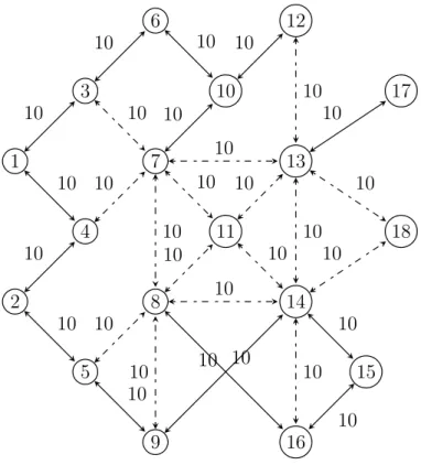
6.1. Small Network . . . 63
6.2. Winnipeg network . . . 66
7. Conclusion and Future Work . . . 70
Acknowledgements . . . 71
Third Article. Benders Decomposition for a Class of Bilevel Programs with Applications to Network Design . . . . 73
1. Introduction . . . 74
2. Benders Decomposition . . . 76
3. Bilevel Uncapacitated Network Design . . . 79
4. Hazmat Transportation Network Design . . . 82
4.1. Literature Review . . . 82
4.2. Applying the Decomposition . . . 83
4.3. Connectivity Cuts . . . 85
4.4. Heuristic . . . 86
5.1. Literature Review . . . 87
5.2. Applying our Decomposition . . . 88
6. Conclusion and Future Work . . . 89
Acknowledgements . . . 90
Conclusion . . . . 91
Limitations and Outlook . . . 92
References . . . . 95
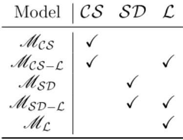
Appendix A. Complete Model Descriptions . . . 101
A.1. Model CS . . . 101
A.2. Model CS-L . . . 102
A.3. Model SD . . . 103
A.4. Model SD-L . . . 104
A.5. Model L . . . 105
Appendix B. Joint Network Design and Pricing . . . 107
B.1. Literature Review . . . 107
B.2. Applying the Decomposition . . . 108
List of Tables
1 Description of the fields in the dataset . . . 32
2 Route choice model estimation results . . . 37
3 Definition of the different MILP reformulations . . . 53
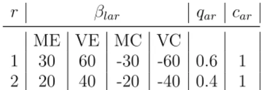
4 Parameters for the two resource types for the small network (αl= 10) . . . 64
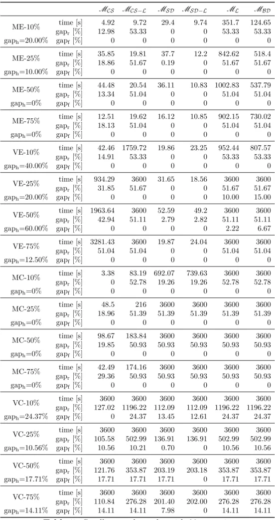
5 Small network results with 30 scenarios . . . 65
6 Parameters for the two types of resources for the Winnipeg network (αl= 0.001) 67 7 Average solution times (5 instances), 50 candidate arcs, 40 OD pairs . . . 67
8 Average results (5 instances with 50 candidate arcs and 40 OD pairs): varying the number of scenarios . . . 70
9 Average results (5 instances with 50 candidate arcs and 40 scenarios): varying the number of OD pairs . . . 71
10 Average results (5 instances with 40 OD pairs and 40 scenarios): varying the number of candidate arcs . . . 71
11 What needs to be solved for cuts on w and Π . . . 82
List of Figures
1 Heat map of the collected data . . . 31
2 Travel paths to access “de Boucherville” port entrance . . . 34
3 Travel time variability to access entrance using path 1, by time of the day . . . 35
4 CO2 emissions in the Port of Montreal . . . 35
5 A small network . . . 63
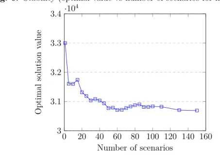
6 Stability (optimal value vs number of scenarios for instance 1) . . . 68
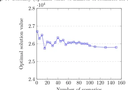
7 Stability (optimal value vs number of scenarios for instance 2) . . . 69
8 Stability (optimal value vs number of scenarios for instance 3) . . . 69
9 Solution times vs number of scenarios . . . 70
List of Acronyms and Abbreviations
GPS Global Positioning System
GMA Greater Montreal Area
OD Origin-Destination
FCP Flow Capture Problem
RUM Random Utility Maximization
LP Linear Program
MIP Mixed Integer Program
MILP Mixed Integer Linear Program
CS Complementary Slackness S D Strong Duality L Lagrangian BD Benders Decomposition ME Mildly Evasive VE Very Evasive MC Mildly Cooperative VC Very Cooperative 17
HTNDP Hazmat Transportation Network Design Problem JNDP Joint Network Design and Pricing
Acknowledgements
First and foremost, I would like to thank my research supervisor Emma Frejinger for guiding me throughout my doctoral studies. Her unwavering diligence greatly contributed to the quality of this work. Her words of encouragement allowed me to persevere through the numerous setbacks that befell our research. Above all however, her kindness and concern for my interests have made the past few years a time I will always look back on fondly.
I am also very grateful to my co-supervisor Bernard Gendron whose expertise provided the impetus behind many developments found in this thesis. His relentless curiosity and rigorous scrutiny of our experimental results gave us valuable insights which further strengthened our research.
I would like to express my thanks to Fabian Bastin as well. In addition to providing very useful feedback in regards to the first article of this thesis, he was the person who originally suggested a PhD with Emma.
Lastly, I must thank my family and friends. Surrounded by them, my life outside of my studies was just as enjoyable as my pursuit of a doctoral degree.
Introduction
This thesis covers the three main following topics: demand model parameter estimation using real GPS data, integrating random utility models into a general flow capture problem and a Benders decomposition specially adapted to a broad class of bilevel models. Throughout this introduction, it is our goal to not only show how these seemingly unrelated subjects lead one into the other, but also the importance of the whole they form. The chapter is structured as follows. First, we showcase the motivation behind this work. Second, we provide a background to the main areas of our research. Third, we lay out our specific objectives and the resulting contributions. Finally, we detail the outline for the rest of this thesis.
Motivation
With the global population more than tripling since the beginning of the 20th century, a need for efficient methods of planning, decision making and simulation came into prominence. This plight was answered by the development of operations research. Owing to the advent of the information age, countless works of ever increasing complexity have been published in a myriad of fields. One of these fields is the study of demand modeling which can be applied to characterizing the behavior of people travelling by choosing one of many alternatives. People and their movements are at the crux of many services, phenomenons and issues such as public transit, air travel, the rise of alternative fuel vehicles, traffic congestion, the concomitant CO2 emissions and other negative impacts. It is thus imperative to accurately
portray the behavior of these people if we are to enact effective policies and take actions entailing environmental and economic benefits. Tracking people with GPS has emerged, in recent years, as a powerful means to that end because of both its quantity and availability. Therefore, providing a way to harness this plentiful resource with the goal of grasping the factors involved in our decision-making processes in regards to our travel choices is of the utmost importance.
However, this undertaking only serves as a basis for determining the choices we make relating to any problematic situation we wish to address. In mathematical programming, decisions are reached by the coalescence of an objective and constraints of which demand
modeling is often a pivotal element. What is typically used in that regard can be greatly improved by simply incorporating state of the art demand models which have evolved sepa-rately. Hence, it beckons to us to unite them with a problem where the behavior of travellers is a central theme. We choose the general flow capture problem as we believe it is a peculiarly versatile setting with numerous concrete applications due to its nature: an authority decides where to install certain flow capturing resources, with the aim of capturing as much traffic as possible, in a network where users, who have a reaction to these resources, are travel-ling. The essence of this situation revolves around the behavior of the travellers and their response to the decisions made by the authority, which, together, dictate the optimal instal-lation configuration. Consequently, incorporating the best representation of the behavior of these travellers in our mathematical program is fundamental.
With a mathematical model able to accurately predict the choices of travellers, the last hurdle which we must clear is that of scaling. Indeed, the unprecedented growth of humanity requires us to consider ever expanding settings which, in turn, translate to extremely large mathematical models. A common approach to circumventing this impediment is the use of heuristics which simplify reality to more manageable dimensions. However, the aptly named decomposition methods deal with the issue by breaking down the problem into smaller parts which can then be addressed efficiently. It is in fact what we use for the general flow capture problem and we demonstrate that our method can be applied to a wide variety of other problems. Thus, the goal is to provide the means for the models used to solve all of these problems to be able to scale up to realistic proportions while simultaneously accurately representing travellers’ behaviors which allows for better decisions.
Research Background
This thesis covers several fields of research and, as such, only the most relevant to this work are discussed here. We also aim to provide, when appropriate, a perspective on what we consider to be a lack of connection between these various topics in the state of the art. Of course, a more thorough overview can be found in the literature review section of each article presented subsequently.
We first look at discrete choice modeling in the context of the path choice of individuals travelling within a network of nodes and arcs. Largely owing their popularity to the seminal work of [54], discrete choice models are used to predict the choices of an individual when choosing from a discrete set of alternatives. This choice is assumed to be based on attributes captured by the utility of the alternatives and characteristics of the individual who is utility maximizing. In reality, for various practical reasons, some of these attributes are unknown to the modeler which leads to random utility discrete choice models. These models determine choice probabilities for each alternative. The probabilities depend on assumptions made regarding the choice set and the random portion of the utility which leads to different models.
This framework naturally lends itself to describe the route choices of individuals travelling within a transportation network. This route choice can be broken down into a series of arc choices leading an individual from his origin to his destination or it can be made from a set of predetermined paths, potentially determined by choice set generation algorithms [e.g, 5, 58].
Both approaches have their strengths and weaknesses. Path-based models have the ad-vantage of being estimated easily by commercial software. They are not conducive to reliable scenario analysis because choice probabilities depend on generated choice sets. These choice sets also have to be recalculated when changes are made to the network. Arc-based models, on the other hand, do not require path choice sets and thus do not suffer from their associ-ated drawbacks. However, they can be limited in their ability to represent certain attributes that are specific to a complete path such as a habitual (preferred) path. More generally, arc-based models require arc-additive attributes which can be a drawback. Nevertheless, it is a widely accepted assumption with respect to shortest path calculations and it is, in fact, often used to generate path choice sets for path-based models. A more detailed overview of the two approaches can be found in [26]. For these reasons, we focus on arc-based models throughout this thesis.
The instantaneous utility of link a ∈ A(k) is u(a|k; β) = v(a|k; β) + ε(a), where A(k) is the set of outgoing links from link k, v(a|k; β) is the deterministic utility and β is a vector of parameters. These parameters typically include the travel time, the speed limit, the road safety, the scenery, etc. The ε(a) represents the random term. These can be assumed to be, for example, independently and identically distributed extreme value (with location zero and scale µ) so that the choice model at each choice stage is logit. One of the most important aspects to consider is the correlation between alternatives. In our context, this translates to different possible paths having certain arcs in common. For instance, a standard logit model does not consider this correlation when calculating path choice probabilities. There are variants of the logit model that address correlation through a correction of the deterministic utilities, such as C-logit [16] and path size logit [6]. However, they rely on a complete path enumeration or choice set sampling [24]. If we define p as a sequence of arcs a1,a2,...,aT, we
can define its associated utility as
u(p) =
T
X
i=2
u(ai|ai−1; β). (1.0)
The probability of choosing path p would thus be given by: Prob(p) = e
v(p)
P
p0∈Pe
v(p0), (1.1)
where P is the set of all paths.
We now turn our attention to random utility models in supply-side mathematical pro-grams. Supply-side problems, in the context of operations research, refer to problems where a manager typically has choices to make in regards to providing services, constructing facil-ities, allocating resources and so on while taking into account the demand. In many cases, discrete choice models that would realistically model the demand are ignored in favor of more simplistic representations. This is mainly due to the non-linear expressions for the choice probabilities of even the simplest discrete choice models as can be seen in Equation (1.1).
Keeping a mathematical program linear is an advantage as it allows to apply the more common solution techniques and thus incorporating choice probability expressions is chal-lenging. These non-linear terms can be approximated in a number of ways: linear functions, piecewise linear functions, or even constants as a compromise [28]. There are also recent developments in conic programming [62]. There is, however, a different and recently de-veloped approach to integrating discrete choice models in mathematical programs which is based on the utilities rather than the probabilities of each alternative. This thesis adopts this approach.
Lastly, we provide a brief overview of bilevel programming as it is one of the focal points in this work. Bilevel problems consist of a leader’s problem and a follower’s problem [17]. The leader is trying to optimize its own objective while respecting certain constraints while the follower does the same with its own objective and constraints as can be observed in (1.2)-(1.5) from [17]. Generally, the decisions of the leader affect the decisions of the follower by changing its objective or constraints. The new decisions of the follower can in turn affect the decisions of the leader. This cycle makes bilevel programs difficult to solve.
min x,y F (x,y), (1.2) s.t. G(x,y) ≤ 0, (1.3) min x f (x,y), (1.4) s.t. g(x,y) ≤ 0. (1.5)
There are many types of solution methods used to deal with bilevel programs [19]. In this thesis, we focus on those that reformulate the bilevel model into an equivalent single-level model through the use of duality theory. This is usually achieved by one of two ways. The first replaces the objective function of the follower’s problem with dual feasibility constraints and complementary slackness conditions. The second substitutes the complementary slack-ness conditions with the strong duality constraint which states that the primal and dual objective functions of a problem are equal at optimality (if a bounded optimal solution exists).
While both of these methods yield mathematical programs that can be solved by standard optimization tools, they have characteristics that may be considered problematic in certain circumstances. Working with complementary slackness conditions means adding a relatively large number of constraints that also have to be linearized which often implies adding a set of binary variables. Although it is a single constraint, the strong duality constraint can have the downside of providing the model with a relatively weak relaxation. Also, in both cases, the structure of the follower’s problem cannot be exactly extracted for a decomposition method because of the additional constraints. However, there is much to gain if we were able to do so. In the context of bilevel network design problems or any other bilevel problem where the follower’s problem consists of finding the shortest path in a network, shortest path problems could be solved very efficiently by algorithms such as the Dijkstra one. This thesis attempts to find a way to obtain a single-level formulation of a bilevel model which would still allow for a decomposition method to benefit from the initial structure of the follower’s problem.
However, simply solving shortest path problems assumes that the followers have perfect knowledge of network attributes and minimize the same objective function. Assuming an uncongested network, for a given origin destination pair, they would hence seek the same shortest path. We can avoid this oversimplification by using the aforementioned advanced discrete choice models. Therefore, the method we use to reformulate a bilevel program to a single-level must be able to use these demand models and preserve the shortest path problem structure so that algorithms can be employed.
Objectives and Contributions
In this section, we explicitly lay out the contributions of this thesis. They are grouped by articles.
The first article, “A GPS-based Recursive Logit Model for Truck Route Choice in an Urban Area”, is centered on calibrating a discrete choice model using real GPS data. The discrete choice model used is a recursive logit model which does not require choice set gen-eration. The contribution is empirical, illustrating how to transition from GPS traces with limited data processing to an estimated set of parameters for the recursive logit model. Furthermore, because the GPS data and the road network used are genuine, the numerical results themselves have value for practical purposes.
The second article, “Flow Capture under Heterogeneous User Behavior in Uncongested Networks”, introduces a new formulation for the flow capture problem. This formulation can accommodate various discrete choice models to represent how traffic propagates in the network. The formulation itself is an important contribution but the key is how a utility simulation approach is adapted to a network context. This approach relies on considering a sufficient number of realizations of arc utilities rather than non-linear probability expres-sions. Another important contribution in this paper is a novel Benders decomposition which
exploits the shortest path problem formulation in the follower’s problem. This is possible because of the particular way in which the bilevel model is brought to a single level without complementary slackness constraints nor the strong duality constraint. The last contribu-tion of this article takes the form of a numerical comparison between the various models developed by the more traditional complementary slackness constraints and strong duality constraint, as well as our Benders decomposition.
The third article, “Benders Decomposition for a Class of Bilevel Programs with Applica-tions to Network Design”, generalizes the decomposition method applied to the flow capture problem in the second article. The first contribution here is the general bilevel model along with the assumptions needed in order to apply our Benders decomposition. This generic model is made more specific by detailing a shortest path problem as the follower’s problem. This allows us to highlight how that structure can be exploited to achieve efficient solution methods. Subsequently, we demonstrate how various bilevel problems can be adapted to fit the form needed for our decomposition. This is done through three concrete examples for which we provide a detailed transition.
To summarize, we first present an application focused on predicting truck route choices using GPS data and the recursive logit model. We then show how it can be adapted into a random utility model used in a bilevel formulation for the general flow capture problem. The resulting formulation can be relatively large, but we demonstrate how a novel Benders decomposition method can be applied to efficiently solve it. Finally, we illustrate that our decomposition can be applied to a wider class of bilevel models dealing with network design and users seeking shortest paths within a transportation network.
First Article.
A GPS-based Recursive
Logit Model for Truck Route
Choice in an Urban Area
by
Léonard Ryo Morin1, Emma Frejinger1, Fabian Bastin1, and Martin Trépanier2 (1) Department of Computer Science and Operations Research and CIRRELT
Université de Montréal, Canada
(2) Department of Mathematics and Industrial Engineering and CIRRELT Polytechnique Montréal, Canada
This article was published as a chapter in Sustainable City Logistics Planning: Methods and Applications, Volume 3. The data analysis project (partly reported in this paper) conducted in collaboration with CargoM, Transport Canada, CIRRELT and several freight carriers was awarded the “Grand prix d’excellence en transport: transport de marchandises” from the Association québécoise des transports (AQTr) in 2017.
My contributions for this paper include handling the data, analyzing it, producing the results and writing the text. Only the code used to estimate the demand model was not mine. Emma Frejinger helped devise the analysis and revised the writing. Fabian Bastin and Martin Trépanier contributed to the writing and provided some useful comments and references.
Résumé.Nous explorons l’usage de données GPS afin d’explorer les chemins qu’empruntent les camions lourds dans le réseau routier urbain de Montréal. L’emphase est mise sur les voyages qui interagissent avec des terminaux intermodaux (gare de triage, port). Nous démontrons que les déplacements des camions peuvent être représentés avec précision et nous proposons un modèle logit récursif pour choix de chemin basé sur ces données. Ceci nous donne une meilleure compréhension des principaux facteurs qui influencent les déci-sions de déplacement et peut potentiellement nous permettre de minimiser les impacts des mouvements des camions, comme les émissions de CO2.
Mots clés : camions lourds, grand réseau urbain, données GPS, choix de route, logit
récursif, terminaux intermodaux, cas d’étude
Abstract.We explore the use of GPS devices to capture heavy truck routes in the Mon-treal urban road network. We emphasize on trips that interact with intermodal terminals (rail yard, port). We show that truck movements can be accurately represented and we propose a recursive logit model for route choice based on this data. This provides a better understanding in the main factors affecting the movement decisions and could potentially offer opportunities to reduce impact on truck movements, such as CO2 emissions.
Keywords: heavy trucks, large urban network, GPS data, route choice, recursive logit,
intermodal terminals, case study
1. Introduction
Moving freight in urban areas is crucial for society and for economic growth. This chapter focuses on the analysis of heavy truck movements between intermodal terminals situated in an urban area. Major intermodal terminals generate a significant amount of traffic and have an important economic value. Ensuring efficient transport to and from these terminals is crucial, not only for the performance of the terminal operations and the trucking companies, but also for reducing the negative impacts of truck traffic, e.g., congestion, noise and emissions. We explore a dataset of GPS traces from multiple large trucking companies active in the Greater Montreal area. These companies are members of an organization called CargoM -Logistic and Transportation Metropolitan Cluster of Montreal. CargoM was in charge of the data collection over three months during the winter of 2013-2014 using 48 GPS loggers.
While mobility patterns of people in urban areas have been extensively studied using GPS data, the literature on its freight counterpart is scarce. Most of the studies analyzing or modeling truck routes using GPS data focus on intercity transport and only a few investigate this problem in urban areas. Moreover, the studies are faced with important data processing challenges. In this study we illustrate through a case study how to generate results useful to stakeholders with only limited data processing. For this purpose, we report both descriptive results and results from structural modeling, in our case, random utility discrete choice models. We use the state-of-the-art methodologies and provide empirical contributions.
The objective of this study is first a descriptive analysis describing heavy truck movements on the island of Montreal and their access times to the two main intermodal terminals (a rail yard in the west and the Port of Montreal in the east) as well as the CO2 emissions on these routes. A second objective is to estimate a route choice model based on map-matched trajectory data. Data processing is typically a time-consuming and error-prone step prior to route choice modeling. The objective of this study is to keep this step to a minimum. Therefore, the descriptive study is based on raw GPS traces where only clearly erroneous data records have been removed. Moreover, the route choice model is link-based and only requires a network representation and map-matched trajectory data, unlike the more commonly used path-based models that require path choice set generation. While the size of the dataset is fairly limited, the main contribution of this study is to illustrate the feasibility of this approach on a large network.
This article is structured as follows. First, we present a brief literature review covering studies of freight movements by trucks using GPS data and discuss route choice modeling in this context. We then present the data followed by the results section. Finally, a conclusion summarizes our findings.
2. Literature Review
Multiple studies have shown the usefulness of GPS data in the analysis of truck movement patterns. GPS data provide a passive way of collecting trajectory data that overcomes the limits of fixed-date freight surveys, knowing that truck movements can vary considerably within weekdays [63]. [52] explores the use of smartphone applications for GPS tracking in order to gather data. GPS data can also be used to complement surveys to provide more information [66, 1, 75]. Truck movements are also subject to heterogeneity in the travel patterns which may be captured by GPS [7].
The main challenges of GPS data analysis often rely on the identification of tours and stops from the GPS traces, as well as information on the transported goods including empty trips. A number of studies [29, 65, 61, 68, 63] have adressed the issue by using various pre-processing methods to remove insignificant trips and by setting thresholds on time spent idle in order to identify a stop. [72] even propose a method to identify tour stops in urban areas with a machine learning algorithm (Support Vector Machine). In our study, the data includes a trip idenfitication number (identified by the driver or by an engine on-off event) which addresses the problem of finding stops within a continuous stream of GPS traces.
[22] propose a method to calculate freight performance measures in corridors. [31] anal-yse the efficiency of truck rail intermodal connectors using travel times for different periods of the week. [44] look at the speed associated to each GPS trace to analyze freight vehi-cle movements around São Paulo. They also analyze the data to identify stops made for deliveries.
While there are many route choice modelling studies focusing on car or public transport choices of individuals, there are relatively few studies on truck route choices. [32] estimate path size and error component models for heavy trucks intercity route choices using the previously described approach using generated choice sets and they provide an analysis of forecasting results. [67] analyze attributes that influence truck routing using a combination of two data sources: interviews at highway truck stops and stated preference data. [35] estimates various decision factors for urban commercial vehicle movements, in particular in the context of vehicle tours.
Most route choice models in the literature are random utility discrete choice models. We focus on this type of model and maximum likelihood estimation of model parameters using revealed preference data (trajectories in real networks). Route choice models are central in many transport applications. For example, the analysis of parameters allows to assess drivers’ preferences towards different types of infrastructure or sensitivity to tolls. Moreover, the estimated models can be used to predict traffic flows. The literature on discrete choice models for route choice analysis can be grouped into three categories: (i) path-based models with generated choice sets of paths that are treated as actual choice sets ([58] provides an overview), (ii) path-based models based on universal choice set (all paths) but where choice sets are sampled and utilities corrected for the sampling [25] (iii) link-based recursive models that are based on universal choice without any choice sets of paths [47]. The third has major advantages over the first two because the model can be consistently estimated without the time-consuming process of choice set sampling and it can be used to compute predicted traffic flows in short computational times [26]. It, however, requires link-additive utilities. In this study, we estimate a recursive logit model [24].
This study uses GPS data to construct a route choice model for trucks in the context of intermodal trips in the Montreal transportation network, where two major logistics centres are present: the port of Montreal and a rail terminal. In doing so, we aim to provide a methodology for not only descriptive GPS data analysis but also route choice model estima-tion in an urban setting.
3. Data and Methodology
In this section, we start by giving a brief overview of the data collection process and the resulting dataset. We then discuss the map-matching procedure followed by a brief description of the recursive logit model.
3.1. Data
The data used in this study was collected on heavy trucks operating during a period of roughly 3 months, between December 9, 2013, and March 4, 2014, in the Greater Montreal
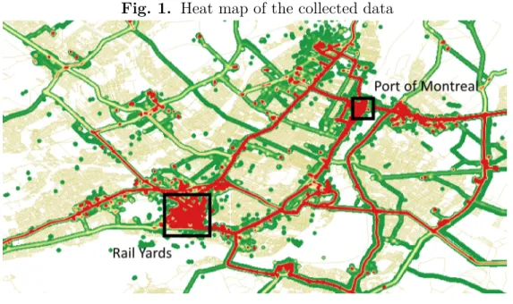
Area (GMA). These vehicles, owned by large trucking companies, primarily moved between the following locations: a major intermodal rail terminal in the center of Montreal Island, intermodal container terminals of the port of Montreal and various warehouses. A data point was recorded for every second when the vehicles’ engine was on. The complete dataset contains 41,569,050 records corresponding to a total of 21,681 trips collected by 48 different vehicles. This gives us an average trip duration of 31.95 minutes which is reasonable given a typical trip length and the road network. Only 0.27% of trip records had invalid values. It is important to note that a new trip is started whenever the engine is switched off or if the driver specifies it through the collecting unit’s interface. This means that many of these so-called trips are not significant both in distance traveled and in number of links used. This issue is dealt with during the map matching process that we discuss in the following section. Figure 1 displays a heat map presenting the density of the data, red indicates a high density of data points while green represents a lower density. Highlighted are the port of Montreal and the intermodal rail yards. Two highways link the two locations and attract significant traffic. Three bridges and a tunnel are used to cross the Saint-Lawrence river running south of the island of Montreal.
Table 1 describes the contents of the GPS dataset, stored in a PostgreSQL database. Apart from the time and geographical information, the dataset also contains information on the cargo weight, provided by the truck driver via a small on-board interface.
Fig. 1. Heat map of the collected data
3.2. Map Matching
In order to estimate a route choice model, we need a description of the road network along with the observed route choices mapped to that network. In our case, all the information
Field Description Example values Survey ID Identification number of the data
recording device.
496, 497, 498 Trip ID Identification number of the
cur-rent trip.
1, 2, 3, 4, 5, 6, 7, 8, 9, 10 Local Datetime Date and time with precision to
the second.
January 10, 2014, 09:24:01 Latitude Latitude in degrees. 45.508928, 45.641103 Longitude Longitude in degrees. -73.509404, -73.762777
Heading Heading in degrees. 78, 186, 278
Wheel based Speed Current vehicle speed (m/s). 10.56, 3.98, 16.13 Cargo Weight Weight of the cargo being
trans-ported currently in various units (when specified by the driver).
0, 20000, 1556
Reason for Stop If specified, number indicating the reason for a stop or the end of the trip.
1, 2, 3, 4, 5, 6, 7, 8
CO2 emissions Instantaneous CO2 emission in g/s.
2.01, 4.37
Table 1. Description of the fields in the dataset
related to the network comes from Adresses Québec (http://adressesquebec.gouv.qc.ca). A Python script is used to extract the relevant information and format it so it can be read in Matlab which is the software we use for route choice model estimation. Observed paths are obtained through a simple map matching algorithm using the data described previously and the road network. While we devised the following simple algorithm taking into account the precision of our GPS records as well as the network data, other algorithms could have been used [59]. First, every record for a single trip is extracted, then a PostgreSQL query assigns a link to each record based on proximity, heading and the direction of the link. The associated link must be within 10 meters of the corresponding GPS traces and their headings can be, at most, 40 degrees apart. If multiple links meet those criteria, then the closest one is retained. Afterwards, this list of links is iterated through by another Python script to build an observed path. At this stage, links must be sequential and certain thresholds are in place to filter out incorrectly matched links. To find an initial link, at least 5 GPS traces must be matched to the same link. Subsequently, a new link is added only when at least 3 consecutive GPS traces match to it. This process is then repeated for each trip. In order to estimate the
recursive logit model, we only keep the 698 observed paths that have a minimum of 6 links because longer trips provide more information.
3.3. Recursive Logit Model
Traditional route choice models represent the alternatives offered to the decision maker as the paths in the network, associating to each path a utility. It is assumed that the drivers aim to maximize their utility, and typically, a logit model is calibrated over the observed path choices. This modeling has, however, two major issues as the feasible paths in a real network cannot be enumerated and we do not know the set of paths actually considered by the decision maker. In addition to potentially long computational times, the obtained estimates can be biased and the predictions inaccurate. The recursive logit model [24] allows to circumvent these issues by assuming that the choice of the path is a sequence of link choices. A link is defined by its source and sink nodes in the network. At each choice stage, the driver chooses from the outgoing links the one that maximizes the sum of the instantaneous utility and the expected maximum utility until the destination (so-called value function). The instantaneous utility of link a ∈ A(k) is u(a|k; β) = v(a|k; β) + ε(a), where A(k) is the set of outgoing links from link k, v(a|k; β) is the deterministic utility and β is a vector of parameters to be estimated. The ε(a) are independently and identically distributed extreme value type I (with location zero and scale µ) so that the choice model at each choice stage is logit. In this context, the value functions are given by the well-known logsum formula and Fosgerau et al. [24] show that they can be computed by solving a system of linear equations. Moreover, the probability of an observed path is the product of the link choice probabilities. The recursive logit model can be estimated and used for prediction without sampling any choice sets of paths as long as path utilities are link-additive and that the path utilities are given as the sum of the deterministic utilities of all links composing the path. We also note that an attribute similar to path size (see [6] for details) can be added to the utilities to correct for correlations. This attribute is called link size. We refer the reader to [24] and the tutorial [77] for more details on the model and its calibration.
4. Results
In this section, we first present an illustrative example of a descriptive analysis of the observed path choices. The scope of the descriptive analysis of the case study was identified by the stakeholders. The descriptive anlysis paved the way to the development of the route choice model, whose results are presented hereafter.
4.1. Descriptive Analysis: Illutrative Example
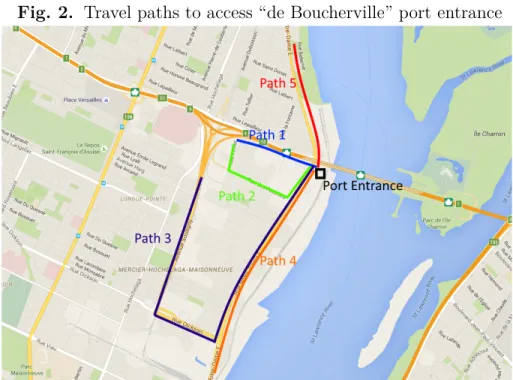
The paths and associated travel times for trips with an intermodal terminal as origin or destination are important as they have an impact on the performance of the trucking oper-ations, in particular, waiting times at the access points. These paths are also of importance for planning the network to avoid queues building up. As an example, Figure 2 illustrates the different street paths that can be used to access the “de Boucherville” entrance of the Port of Montreal.
Fig. 2. Travel paths to access “de Boucherville” port entrance
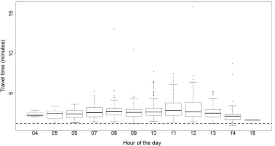
In our data, we observed a total of 1,131 entries made to the port at this location. The most used paths are path 1 (60.7% of occurrences) and path 4 (11.4%) while the other three paths are not significantly used (a combined 3.8%). The remaining 24.1% of entries could not be matched to any of the five paths. This is explained by the fact that these vehicles stopped at the warehouses in the area between paths 1 and 2 for some time before making a technically new trip to the port entrance. Since path 1 is the only path with a significant number of observations, we present a more detailed analysis of its travel times in Figure 3. The travel times slowly increase during the morning. More variability is observed from 10:00 to 13:00, a “peak” period for the port activities. This is reflected in the relatively high number of outliers and in the top whisker (the “maximum”). The dotted line indicates the travel time while driving at the legal speed limit. A similar analysis has been done for the exits from the port. It has contributed in enhancing traffic management at the “de Boucherville” exit: traffic signal timings have been changed to improve the situation.
Fig. 3. Travel time variability to access entrance using path 1, by time of the day
Fig. 4. CO2 emissions in the Port of Montreal
We also conduct an analysis of CO2 emissions in the Port of Montreal as a function of the time of day. First, we note that a small percentage of observations have a missing instantaneous CO2 emission value despite registering a movement speed above 0 m/s. There are different ways to impute these missing values. In our case, there are relatively few missing values so we use a crude method where we simply impute an average value from the observations, 2.05 g/s. Figure 4 reports the observed average emissions in kilograms over the time of day. We separate the results for observations with and without imputed values.
Furthermore, 4,836,698 records, representing 60.2% of the 8,034,382 records that are located within the area of the port, have a movement speed registered at 0 m/s. This means that the vehicle is not moving but has the engine on (idling). Summing the emissions for these observations, we have 8.9 tons of CO2 from stationary vehicles over the course of the 3 months during which the data was collected. Of course, for this number to have any meaning, we must calculate the percentage of the total number of trucks entering the port our sample represents. Using the number of trucks entering the port per day in our data and the real number recorded by port authorities, we estimate that our dataset represents 1.46% of all traffic. If we extrapolate using these numbers, idling vehicles emitted up to 550 tons of CO2 during the 3-month period. This brings us to develop a path choice model to, in the end, better understand the behavior of the drivers. These insights and route choice predictions can be used to improve the infrastructure to reduce the emissions.
4.2. Recursive Model Estimation
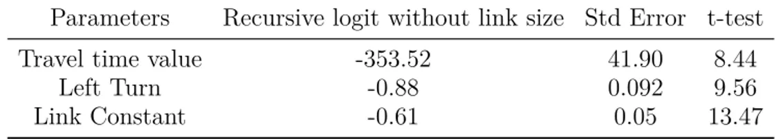
In this section, we present the estimation results of the recursive logit model without link size. The model is based on a large network containing 215,403 links and 115,157 nodes covering the whole region of the observations. The utilities are linear-in-parameters and are a function of the three following attributes: travel time (TT), link constant (LC) and left turns (LT). We recall that these utilities are link-additive. The deterministic part of the utility of an arc a is defined as v(a|k; β) = βTTT T (a) + βLTLT (a|k) + βLCLC(a). So, the
path travel time is the sum of the link travel times, left turns correspond to the number of left turns in a path and the path interpretation of link constant is the number of crossings. Based on statistical testing (t-test and likelihood ratio test), we analyzed different attributes and model specifications. Here, we report the model with the best in-sample fit.
We use an open-source Matlab code (https://github.com/maitien86) to estimate the model by maximum likelihood. It is an implementation of the nested fixed point algorithm proposed by [39], used in [47]. We can estimate the recursive logit model in a relatively short computational time using the decomposition method developed in [46]. There is an additional time required to load the data in Matlab, however, this loading time is also short (the computations were done on a machine with an i7 processor and 12 GB of RAM running Debian 3.16; the loading time is approximately 30 minutes and the run time is around 20 minutes). The computational time for the link-size model is longer because the utilities become origin-destination specific and the decomposition method cannot be used.
The estimation results are reported in Table 2. We note that the parameter estimates have their expected signs (negative) and they are significantly different from zero. This implies that an increase in expected travel time and left turns decreases the overall utility. The relatively high magnitude of the travel time parameter can be explained by the fact that the unit of time is in hours. Therefore, expected travel time values in hours for any link
would be quite small and, when multiplied by the travel time parameter, would not simply overtake every other parameter. In fact, we can interpret the ratios of the parameters relative to each other: 0.88/ 353.52 = 0.002. This means that a left turn is equivalent to adding 0.002 hours, or 8.95 seconds, to the travel time in our average truck driver’s perception of route choice. Applying the same logic to the link constant parameter, which represents crossings, we have that a single crossing is equivalent to 6.24 seconds of additional travel time.
The purpose of our case study was to analyze in-sample results and, in that regard, the results are satisfactory. We note that the estimated model can be used to simulate truck route choices between different OD pairs and to compute traffic flows using an OD matrix as input in short computational times similar to [78].
Parameters Recursive logit without link size Std Error t-test
Travel time value -353.52 41.90 8.44
Left Turn -0.88 0.092 9.56
Link Constant -0.61 0.05 13.47
Table 2. Route choice model estimation results
5. Conclusion and Future Work
In this chapter, we analyzed truck drivers route choice behavior in two ways. First through a descriptive analysis based on raw GPS data and second, through the estimation of a recursive logit model. While the dataset is too small to draw general conclusions for the population of truck drivers in the Montreal region, the results illustrated that insights can be gained with a limited data processing effort. This holds true in particular when the interest lies in analyzing a specific region of the network, in our case the entry paths to the Port of Montreal. We also illustrated that the recursive logit model can be applied in a very large network. The model has the advantage of not requiring any generation of path choice sets, which is typically a time-consuming and error-prone part of route choice modeling. Future research should be dedicated to the analysis of truck tours, an aspect that we have ignored in this study since the focus was set on trips with one of the intermodal terminals as origin or destination.
Acknowledgements
The authors wish to acknowledge the funding and the support of CargoM, the logistics and transportation cluster of Montreal, for providing the data used in this study. We are grateful to Tien Mai for helping us with his MATLAB code used for the recursive logit model estimation. This research was partially funded by the National Sciences and Engineering Research Council of Canada, discovery grant 435678-2013.
Second Article.
Flow Capture under
Heterogeneous User Behavior
in Uncongested Networks
by
Léonard Ryo Morin1, Emma Frejinger1, and Bernard Gendron1
(1) Department of Computer Science and Operations Research and CIRRELT
Université de Montréal, Canada
This article will be submitted to Operations Research before the thesis defense.
My contributions for this paper include implementing and refining the various models, devising the numerical experiments, producing the results and writing the text. Emma Frejinger helped detailing the theory around discrete choice. Bernard Gendron provided the initial mathematical developments leading to the Benders reformulation. Both Emma Frejinger and Bernard Gendron helped rewrite and reorganize certain sections.
Résumé.Nous considérons le problème de capture de flot dans lequel un gérant de réseau de transport décide sur quels arcs installer des ressources qui interceptent le trafic tout en affectant leurs chemins. Dans l’état de l’art de ce problème, les flots de trafic sont déterminés par des hypothèses simplistes comme des utilités déterministes et des ensembles de choix. Notre première contribution est une formulation qui incorpore un modèle stochastique d’af-fectation de trafic basé sur les arcs qui présume que les usagers font des choix maximisant des utilités aléatoires. Ceci permet de prendre en compte une variété de préférences in-cluant différentes perceptions des resources (positive, indifférente, négative). Pour obtenir cette formulation, nous proposons un programme biniveau à partir duquel nous dérivons plusieurs formulations dites “mixed integer linear”. À partir d’une d’entre elles, obtenue en utilisant la dualité forte de manière particulière, nous dérivons une nouvelle méthode de dé-composition de Benders. Notre seconde contribution est cette dédé-composition. Finalement, nous menons des expériences numériques sur un grand réseau afin de démontrer que des instances relativement grandes peuvent être résolues en un temps raisonnable.
Mots clés : Problème de capture de flot, comportement d’usagers, choix de chemin
sto-chastique, logit récursif, décomposition de Benders
Abstract.We consider the general flow capture problem where a transportation network manager decides on which arcs to locate traffic intercepting resources that affects traffic flows. In the current state of the art surrounding this problem, traffic flows are determined under simplistic hypotheses such as deterministic utilities and path choice sets. Our first contribution is a formulation which integrates an arc-based stochastic traffic assignment model based on the assumption that travellers make random utility maximization choices. This allows to account for a variety of preferences, including different perceptions (positive, indifferent or negative) of the resources. To reach this formulation, we propose a bilevel program from which we derive several general mixed integer linear program formulations. From one of them, which is obtained through an uncommon use of strong duality, we derive a novel Benders reformulation. Our second contribution consists of this particular decom-position method. Finally, numerical experiments conducted on a large network show that relatively large instances can be solved in reasonable times.
Keywords: Flow capture problem, user behavior, stochastic path choice, recursive logit,
Benders decomposition
1. Introduction
Flow capture problems (FCPs) concern the decisions on where to locate resources in a network so as to capture traffic flows. They can be viewed as facility location problems with the distinguishing feature that demand is represented by traffic flows as opposed to being static in specific locations. The objective of FCPs, subject to various constraints (e.g., budget), can be expressed, for example, as maximizing the amount of captured flow or as minimizing the consequences of non-captured flows. FCPs form a broad class of problems and encompass a variety of applications such as optimal location of rail park-and-ride facilities [34, 41], vehicle inspection stations [27, 55] and alternative fuel stations [60, 45, 42, 71].
[4] propose to categorize FCPs into three classes based on the assumption on the traf-fic flows in regards to the presence of resources. We refer to these classes as indifferent,
cooperative or evasive flows. Cooperative and evasive flows clearly depend on the resource
location decisions as the former seek them out, while the latter avoid them. These traffic flows are a result of travellers’ route choice behavior where they seek to minimize their in-dividual generalized cost function. This is known as the traffic assignment problem: given an origin-destination (OD) matrix containing the number of trips between each origin and destination in the network, and given a route choice model, the traffic flows are computed assuming that the travel time is either a function of the traffic volume or is constant (i.e., no congestion). In this work, we take the latter point of view, which is consistent with the state of the art on FCPs (see Section 2).
Our contribution, however, significantly extends the state of the art, as the FCP models proposed in the literature are based on the assumption that travellers behave in a known and deterministic way, that is, travellers minimize a perfectly known generalized cost function so the route choice problem is reduced to a simple shortest path problem. There is a large gap between this strong assumption and the state of the art in route choice models. In fact, there is ample empirical evidence in the literature focused on route choice analysis [77] that travellers’ generalized cost functions cannot be known perfectly. In turn, this motivates the use of random utility maximization (RUM) models, which have better prediction accuracy. Moreover, the spatial overlap of paths in a transportation network requires RUM models that allow utilities to be correlated. The simplest RUM model – logit, aka logistic regression – is based on the assumption that utilities are uncorrelated and has a poor prediction per-formance compared to models that allow for correlated utilities. Most network optimization formulations that integrate user behavior use a logit model (see Section 2). Note that, even this simplest setting leads to non-linear non-convex formulations.
We aim to fill the gap between the state of the art on FCPs and route choice models. This paper offers four main contributions:
(1) We propose a bilevel programming model for the FCP where the lower-level route choice decisions are given by an arc-based RUM model, called nested recursive logit [47]. It allows to predict traffic flows without any enumeration of choice sets of paths – i.e., the support for the probability distribution – and path utilities that are correlated. By appropriately defining the utility functions, the model can predict traveller behavior according to any class of flows – evasive, cooperative or indifferent – and accounts for the heterogeneous behavior within each class.
(2) Based on the simulation approach proposed in [56], we express the RUM model in arc utility space instead of arc probability space. On the one hand, this leads to linear constraints instead of non-linear ones. On the other hand, the resulting model has
a large number of variables and constraints. This is particularly challenging in our case as, unlike [56], we focus on the more complex network optimization setting. (3) The bilevel programming model is rewritten as a single-level model through the
ad-dition of a Lagrangian term derived from strong duality constraints as opposed to simply including them as constraints or by including complementary slackness con-straints. The structure of the resulting model can be exploited to devise an efficient Benders decomposition that relies heavily on solving shortest path problems rather than linear programs, thus allowing large instances to be solved in reasonable times. (4) We present results from extensive computational experiments on both a small illus-trative network and the larger Winnipeg network, commonly used as a benchmark for evaluating traffic assignment models [e.g., 3, 57, 37, 38]. Experiments on the small network allows us to assess the impact of various problem characteristics and to test the scalability of the single-level models when solved with a state-of-the-art solver, thus motivating the use of Benders decomposition for the larger Winnipeg network. The remainder of the paper is structured as follows. Section 2 contains a review of the relevant literature. Section 3 describes the problem and the bilevel programming formulation integrating the simulation approach. Section 4 details various techniques to achieve single-level formulations, which are then linearized in order to exploit state-of-the-art mixed-integer linear programming (MILP) solvers. Section 5 presents the Benders decomposition method. Section 6 focuses on our numerical experiments, while Section 6 concludes the paper and proposes avenues for future research.
2. Literature Review
This chapter is focused on bridging the gap between the state of the art in demand modeling – in this case route choice behavior – and network optimization for FCPs. There are two aspects capturing the demand in any FCP formulation. First, there is what we refer to as aggregate demand, the number of trips between each OD pair over a given period of time, captured in an OD matrix. Second, there is how these trips are distributed over paths in the network in response to the resource allocation decisions. We refer to this as disaggregate demand. Most studies on FCPs are single period, however [51] consider a multi-period problem. Aggregate demand is assumed to be fixed and given with a notable exception in [71] where aggregate demand is stochastic. Accordingly, we focus on a single period problem assuming deterministic aggregate demand. Our contribution focuses on integrating state of the art disaggregate demand models. In the following we provide an overview of disaggregate demand models in the context of FCPs. We then review the state of the art in RUM route choice models followed by a high-level description of bilevel programming models where the lower-level user response is given by a RUM model. Finally, we describe the simulation approach of [56] on which we base this work.
Disaggregate demand is incorporated into FCPs in various ways across the literature. In the seminal works of [33] and [8], the demand is assumed to travel along the predetermined shortest path for each OD pair. The concept of deviation, where users are willing to deviate from the shortest path to seek out or avoid a facility, is integrated in several subsequent works [e.g., 74, 42, 50]. This is mainly done through path set enumeration, which implies a limitation in regards to the number of paths considered. More recently, [4] improved on this by reworking the model proposed in [50] to dynamically find the shortest path with an arc-based formulation. However, their model remains deterministic similarly to the path enumeration approaches. To the best of our knowledge, there are no RUM models used to represent the disaggregate demand in FCPs, which is the gap we address in this work.
RUM models are frequently used to analyze and to predict route choice behavior in transportation networks. There are two key challenges in this context that have been ex-tensively studied: (i) the definition of choice sets and (ii) modeling correlated utilities in a computationally tractable manner. Recursive models proposed by [24], [47] (aka maximum entropy inverse reinforcement learning) [76] address these challenges. We refer to [77] for a comprehensive overview of related work. Based on dynamic programming, these models predict path choices based on an arc formulation without any restrictive assumption about the choice sets, that is, any feasible path in the network is part of the choice set. We explore this nice property.
While RUM models have not been included in FCPs, they have been integrated in other problems. An example is the logit network pricing detailed in [28]. The solution approach consists of solving a linear approximation of the problem and then using a local search method. There are three possible approximations presented in their work. The first consists of using a deterministic path assignment. The second and third consist of replacing the non-linear term describing the choice probability of each alternative by a constant function and a linear function, respectively. [49] consider a facility location problem with a RUM (logit) model to calculate choice probabilities. A heuristic based on GRASP (greedy randomized adaptive search procedure) and tabu search is proposed. Using [49] as a starting point, [20] reformulate the model as a bilevel program with endogenous facility service rate variables amongst its improvements. Their solution method is a heuristic based on that of [28].
An alternate method of incorporating a RUM model, the one we use in our work, is based on the simulation approach of [56]. They propose to integrate a sample average ap-proximation of predictions from discrete choice models into MILP formulations. Instead of working with the non-linear expressions representing choice probabilities, the approach focuses on drawing random terms from the distribution of the choice model to obtain utility values. Following a principle of utility maximization, user choices correspond to the alter-natives having maximum utility. This approach, to our knowledge, has not yet been used in
a network optimization context, which exhibits specific challenges compared to the setting considered by [56].
In summary, the gap we address in this paper is the lack of RUM models in the FCP literature. This is achieved by adapting a simulation approach to a network optimization setting, which is also a new development. The resulting bilevel programming formulation is presented in the following section.
3. Problem Description and Bilevel Model
In this section, we introduce the FCP that we consider in our work, along with a bilevel programming model. In this context, the decision maker chooses where to locate different types of resources r ∈ R on the arcs of an uncongested network G = (N,A) composed of nodes n ∈ N and arcs a ∈ A. The resources available on each arc a ∈ A are identified with the indicator parameter σar that takes value 1, if resource r ∈ R can be installed on arc a ∈ A,
and value 0, otherwise. Note that we might have P
r∈Rσar = 0, in which case arc a ∈ A
cannot be used to locate any resources. The objective is to maximize the overall captured traffic flow. Associated with each arc a ∈ A and each resource r ∈ R is an installation cost
car > 0 and a proportion of the flow the resource can capture qar ∈ (0,1]. The decisions
may be subject to different constraints, such as, not exceeding an overall budget b > 0, and imposing a maximum or a minimum number of resources to install on subsets of the arcs. For the sake of simplicity, we only impose the constraint that a single resource can be installed on each arc. The resource location decision variables yar are equal to 1, if a resource of type
r ∈ R is installed on arc a ∈ A, and to 0, otherwise. We then assume the constraints on the
resource location variables to be captured by set
Y = ( y ∈ {0,1}|A|×|R|| X a∈A X r∈R σarcaryar ≤ b; X r∈R σaryar ≤ 1, a ∈ A ) .
Accordingly, in the remainder of the paper, we write these constraints in the compact form
y ∈ Y .
Users observe the location of the resources and make route choices between different OD pairs k ∈ K according to their preferences. For example, they can be attracted to the resources (henceforth cooperative users), indifferent to them, or they might want to avoid them (henceforth evasive users). They can also have different preferences regarding other characteristics of the network, such as distance, presence of traffic lights, specific road types and speed limits.
As the objectives of the decision maker and the users are not necessarily aligned, the problem can be formulated as a bilevel program where the leader is the decision maker and the followers are the users of the system. We divide the users into categories l ∈ L depending on their preferences and type of behavior. Also, we assume that the aggregate demand is