HAL Id: hal-02136901
https://hal.archives-ouvertes.fr/hal-02136901
Submitted on 22 May 2019
HAL is a multi-disciplinary open access
archive for the deposit and dissemination of
sci-entific research documents, whether they are
pub-lished or not. The documents may come from
teaching and research institutions in France or
abroad, or from public or private research centers.
L’archive ouverte pluridisciplinaire HAL, est
destinée au dépôt et à la diffusion de documents
scientifiques de niveau recherche, publiés ou non,
émanant des établissements d’enseignement et de
recherche français ou étrangers, des laboratoires
publics ou privés.
From non parametric statistics to speech denoising
Dominique Pastor, Asmaa Amehraye
To cite this version:
Dominique Pastor, Asmaa Amehraye. From non parametric statistics to speech denoising. ISIVC
2006 : 3d international symposium on image/video communications over fixed and mobile networks,
Sep 2006, Hammamet, Tunisia. �hal-02136901�
FROM NON-PARAMETRIC STATISTICS TO SPEECH DENOISING
Dominique Pastor
1, Asmaa Amehraye
1,
21GET - Ecole Nationale Sup´erieure des T´el´ecommunications de Bretagne
Technopˆole de Brest Iroise, 29238 BREST Cedex, France,
{dominique.pastor,asmaa.amehraye}@enst-bretagne.fr
2GSCM-LEESA Facult´e des Sciences de Rabat,
4 Avenue Ibn Battouta B.P. 1014 RP, Rabat, Maroc
ABSTRACT
Given some signal additively corrupted by independent white Gaussian noise with unknown standard deviationσ,
we present a new estimator of σ. This estimator derives
from a theoretical result presented and commented in the paper. Without any preliminary signal detection, the esti-mate is performed on the basis of the time-frequency com-ponents returned by a standard spectrogram where the Dis-crete Fourier Transform is simply weighted by the square window. No assumption about the signal statistics is made. The signal time-frequency components are assumed to have probabilities of presence less than or equal to one half.
This estimator is suited to speech denoising. It avoids the use of any Voice Activity Detector and is an alternative solution to subspace approaches. Objective performance measurements show that the standard Wiener filtering of speech signals can be tuned with the outcome of this es-timator without a significant loss in comparison with the measurements obtained when the noise standard deviation is known.
1. MOTIVATION
Lets[t], t = 1, . . . , T be the samples of some speech
sig-nal and suppose that theseT samples are corrupted by
ad-ditive and independent stationary noisex[t], t = 1, 2, . . . , T
so that the samples of the observed signal are
y[t] = s[t] + x[t], t = 1, . . . , T. (1) We assume that noise is white and Gaussian with null mean and standard deviation σ: for every t ∈ {1, 2, . . . , T }, x[t]∼ N (0, σ2).
The Wiener filtering of the noisy speech signaly
re-quires prior knowledge of the noise standard deviationσ.
A basic and popular solution consists in using a Voice Ac-tivity Detector (VAD): the estimate ofσ is the square root
of the Maximum Likelihood Estimate (MLE) computed on the basis of the samples of the time frames that the VAD has detected as noise alone. Subspace approaches can also be used to estimateσ by computing the smallest
eigenvalues of the noisy speech autocorrelation matrix; the model order is difficult to choose and the computation of the eigenvalues may prove unstable.
This paper proposes a new estimator of the noise stan-dard deviation. The theoretical foundation of this estima-tor is proposition 3.1, stated in section 3 after exposing some preliminary material in section 2. This theoretical result is non-parametric in the sense that it makes no as-sumption about the probability distributions of the signals and assumes neither that these signals are identically dis-tributed nor that they have equal probabilities of presence. Section 4 then presents the estimator deriving from proposition 3.1 and a few preliminary experimental re-sults. This estimator is then employed in section 5 to ad-just the standard Wiener filtering of the noisy speech signal
y introduced above. According to objective performance
measurements, the denoised speech signals are not signif-icantly more distorted than those achieved when the fil-tering is tuned with the exact value of the noise standard deviation.
Conclusions and perspectives are given in section 6.
2. PRELIMINARY MATERIAL
The random vectors and variables are supposed to be de-fined on the same probability space denoted by(Ω,M, P )
and for every elementω ∈ Ω. As usual, if property P
holds true almost surely, we writeP (a-s).
Given a positive real valueσ, a sequence X = (Xk)k∈N
of random complex variables is said to be a complex white Gaussian noise (CWGN) with standard deviationσ if the
random variablesXk,k = 1, 2, . . ., are complex, mutually
independent and identically Gaussian distributed with null mean and varianceσ2. The real and imaginary parts
ℜXk
andℑXkof eachXkform a two-dimensional random
vec-tor such that(ℜXkℑXk)∼ N¡0, (σ2/2)I¢where I stands
for the2× 2 identity matrix.
The minimum amplitude a(S) of a sequence S = (Sk)k∈N
of random complex variables is defined by
a(S) = sup{α ∈ [0, ∞] : ∀k ∈ N, |Sk| ≥ α (a-s)} . (2)
Iff is some map of the set of all the sequences of complex
random variables into R, we say that the limit off is ℓ∈ R when a(S) tends to∞ and write that lima(S)→∞f (S) = ℓ if, for any positive real value η, there exists some A0 ∈ (0,∞) such that, for every A ≥ A0and everyS such that a(S)≥ A, |f(S) − ℓ| ≤ η.
The setL2(Ω, C) stands for the set of those complex
random variablesY such that E[|Y |2] <∞. We then
de-fineℓ∞(N, L2(Ω, C)) as the set of those sequences S = (Sk)k∈N of complex random variables such that Sk ∈ L2(Ω, C) for every k∈ N and sup
k∈NE[|Sk|2] is finite.
Given a random variableY and a real number τ ,I(Y ≤ τ ) stands for the indicator function of the event{Y ≤ τ}.
As usual,I0 is the zeroth-order modified Bessel function
of the first kind. Throughout the rest of the text, we say ’in-dependent’ instead of ’mutually in’in-dependent’ for brevity.
3. A THEORETICAL RESULT
Proposition 3.1 stated below is a corollary of a more gen-eral theorem established in [6]. As an introduction to propo-sition 3.1, we begin with an intuitive approach. It makes the reader understand the main ideas behind proposition 3.1 and the results given in [6].
Consider a sequenceY = (Yk)k∈N of complex
ran-dom variables where each Yk is either the sum of some
signal Sk and noiseXk or noiseXk alone. We assume
that X = (Xk)k∈N is a CWGN with standard deviation σ. For every given k ∈ N, the presence of noise alone
is the null hypothesis whereas the presence of some signal in noise is the alternative one. We assume that, for ev-eryk ∈ N, the index of the true hypothesis is a random
variableε, valued in{0, 1} and independent with Skand Xk. We thus can write that Yk = εkSk + Xk. The a
priori probabilities of presence and absence of the signal
Λkare thenP ({εk = 1}) and P ({εk = 0}), respectively.
Proposition 3.1 significantly reduces the importance of the choice of these probabilities since they will be assumed to be upper-bounded.
At this stage, assume that the random variables εk, k ∈ N, are independent and identically distributed (iid)
as well as the random signalsSk,k∈ N. It follows that
the random vectors Yk, k ∈ N, are iid as well. Let p
stand for the common value of the probabilities of pres-enceP ({εk= 1}). We assume that p ≤ 1/2.
Given some real numberT , set Am(T ) = 1 m m X k=1 |Yk|I(|Yk| ≤ T )
According to Kolmogorov’s classical strong limit theorem,
lim
m→∞Am(T ) = E [|Yk|I(|Yk| ≤ T )] (a-s) (3)
wherek is any element of{1, . . . , m}. An easy
computa-tion shows that we can write that
E [|Yk|I(|Yk|≤T )] = (1−p)E [|Xk|I(|Xk|≤T )] × µ 1+ p 1− p E [|Sk+Xk|I(|Sk+Xk|≤T )] E [|Xk|I(|Xk|≤T )] ¶ . (4)
LetA be a lower bound for the amplitudes of the signals Sk,k ∈ N. If A is large enough in comparison with σ,
we can reasonably expect the existence of some threshold
T that makes it possible to distinguish noisy signals from
noise alone with a rather small probability of error. As a
matter of fact, regarding the choice forT , we can be very
specific as follows.
For any given non negative real numberh, letTτstand
for the map defined for every complex valuez by Tτ(z) =
½
1 if|z| ≥ τ
0 otherwise. (5) Clearly, for everyk∈ N, Tτ is a statistical test for
mak-ing a decision on the value ofεk since the composite map Tτ(Uk) is measurable andTτ(Uk)∈ {0, 1}. In what
fol-lows,Tτis called the thresholding test with threshold height τ . The error probability of this test is then the probability P ({Tτ(Uk)6= εk}) of the event {Tτ(Uk) 6= εk}. This
error probability does not depend onk since the
observa-tionsUk,k∈ N, are assumed to be iid. This is the reason
why we simply denote it byPe{Tτ}, without mentioning
the observation under consideration.
Since the probability of presence of any signalSk,k∈ nN, is assumed to be less than or equal to 1/2 and by
taking into account that (see [1, Eq. 9.6.47, p. 377])
I0(x) =0F1(1; x2/4), [4, Theorem VII.1] tells us the
fol-lowing. For everyx∈ R, set κ(x) = I0−1(ex
2
)/2x (6)
with κ(0) = 1; for making a decision on the value of εk where k is any natural number, the error probability Pe{Tσκ(A/σ)} of the thresholding test Tσκ(A/σ)with
thresh-old heightσκ(A/σ) is less than or equal toQ(A/σ) where,
for any given non-negative real numberx, Q(x) = e−x2Z κ(x) 0 e−t2 tI0(2xt)dt + 1 2e −κ(x)2 . (7)
We thus can write thatPe{Tσκ(A/σ)} ≤ Q(A/σ). In
equa-tion (4), set nowT = σh with h = κ(A/σ). The function Q(x) decreases very rapidly when x increases. Hence, for
large values ofA, the probabilities P ({|Xk| > σh}) and P ({|Sk+ Xk| ≤ σh}) are small and, thus, the expectation E [|Sk+ Xk|I(|Sk+ Xk| ≤ σh)] can reasonably be
ex-pected to be significantly smaller thanE [|Xk|I(|Xk| ≤ σh)].
Since p is assumed to be less than or equal to one half, p/(1− p) is less than or equal to 1. Consequently, in a
certain sense to specify, we should be able to prove that
E [|Yk|I(|Yk| ≤ σh)] ≈ (1 − p)E [|Xk|I(|Xk| ≤ σh)] .
Without caring about mathematical exactness, we com-bine this approximation to the almost surely convergence of equation (3) to obtain that, in a certain sense,
Am(σh)≈ (1 − p)E [|Xk|I(|Xk| ≤ σh)] (8)
whenm and the amplitudes of the signals are both large.
If we now setBm(T ) = m1 Pmk=1I(|Yk| ≤ σh), the
same type of intuitive approach suggests that
Bm(σh)≈ (1 − p)E [I(|Xk| ≤ σh)] . (9)
Consider now the ratio Am(σh)/Bm(σh). This
Moreover, sinceXk ∼ Nc(0, σ2), the distribution of|Xk|
is known and its density f (x) is that of the square of a
Rayleigh distributed variable. Taking into account that the variance of the real and imaginary parts ofXkboth equal σ2/2, this density is given by :
f (x) = ½
(2x/σ2)e−x2/σ2
ifx≥ 0,
0 otherwise. (10)
Therefore, we easily obtain thatE [|Xk|I(|Xk| ≤ σh)] = 2σR0ht2e−t2
dt and that E [I(|Xk| ≤ σh)] = P ({Xk ≤ σh}) = 1−e−h2
. According to these equalities, equations
(3) and (8), we conclude that
Am(σh)/Bm(σh)≈ 2σ Z h 0 t2e−t2 dt/(1− e−h2 ). (11)
Once again, this approximation must be understood with respect to a certain convergence criterion. This one is introduced in proposition 3.1. Its more general form is given in [6]. As a matter of fact, the same type of intuitive approach as that presented above can be used to guess part of the results established in [6]. Proposition 3.1 and its extension not only specify the exact meaning of equation (11) but also significantly extend the conditions of validity of (11) because they state that the convergence holds true even for non iid signals and non iid priors.
Proposition 3.1 LetY = (Yk)k∈Nbe a sequence of
com-plex random variables such that, for everyk ∈ N, Yk = εkSk+ Xk whereS = (Sk) ∈ ℓ∞(N, L2(Ω, C)), X = (Xk)k∈Nis a CWGN with standard deviationσ and ε = (εk)k∈Nis a sequence of random variables valued in{0, 1}
respectively.
Assume that
(A1) for everyk∈ N, Sk,Xkandεkare independent;
(A2) the random variablesYk,k∈ N, are independent;
(A3) the random variablesεk,k∈ N, are independent;
(A4) the priorsP ({εk = 1}), k ∈ N, are less than or
equal to one half.
Given any natural numberm and any pair (x, T ) of
positive real numbers, define the random variableDm(x, T )
by Dm(x, T ) = ¯ ¯ ¯ ¯ ¯ ¯ ¯ ¯ ¯ ¯ m X k=1 |Yk|I(|Yk| ≤ xT ) m X k=1 I(|Yk| ≤ xT ) − 2x Z T 0 u2e−u2du 1− e−T2 ¯ ¯ ¯ ¯ ¯ ¯ ¯ ¯ ¯ ¯ .
Then, the standard deviationσ is the unique positive
real numberx such that, for every β0∈ (0, 1], lim a(S)→∞ ° ° °limm Dm(x, βκ(a(S)/x)) ° ° ° ∞= 0 (12)
uniformly inβ∈ [β0, 1] where, for every x∈ R, κ(x) = I0−1(ex
2
)/2x (13)
withκ(0) = 1.
4. A NEW ALGORITHM FOR ESTIMATING THE NOISE STANDARD DEVIATION
On the basis of proposition 3.1, we start by introducing a discrete cost. A minimum of this discrete cost can be computed and considered as a first estimate of the noise standard deviation. This estimate will be called the Es-sential Supremum Estimate of typeI (ESE-I) because of
the crucial role played by the essential supremum norm in its computation. The term ESE-I will also stand for the
estimator itself.
Experimental results aimed at assessing the ESE-I
sug-gest another estimate of the noise standard deviation. This new estimate is hereafter called the Essential Supremum Estimate of typeII (ESE-II). The term ESE-II will also
designate the estimator itself. According to Monte-Carlo experiments of the same type as those mentioned above, the ESE-II performs better than the ESE-I.
4.1. The ESE-I
Let L be some natural number and set βℓ = ℓ/L, ℓ = 1, 2, . . . , L. Suppose that A is some known lower bound
for the amplitudes of the signal. We thus have a(S) ≥ A. These new notations are kept hereafter with the same
meaning.
Considerm observations Y1, Y2, . . . , Ym. IfA and m
are large enough, proposition 3.1 suggests estimating the noise standard deviation by a possibly local minimum of
sup ℓ∈{1,...,L}{D
m(x, βℓκ(A/x))} (14)
whenx ranges over a suitable search interval. However,
in practice, no lower bound for the amplitudes of the sig-nals is known. Surprisingly enough since 3.1 states that the largerA the better the estimate, the experimental
re-sults presented in [5] and [6] suggest that the asymptotic condition on the minimum amplitude of the signals can be relaxed significantly. Therefore, we consider the trivial lower boundA = 0 and the discrete cost we minimize is
then sup ℓ∈{1,...,L} ¯ ¯ ¯ ¯ ¯ ¯ ¯ ¯ ¯ ¯ m X k=1 |Yk|I(|Yk| ≤ xβℓ) m X k=1 I(|Yk| ≤ xβℓ) − 2x Z βℓ 0 u2e−u2du 1− e−β2 ℓ ¯ ¯ ¯ ¯ ¯ ¯ ¯ ¯ ¯ ¯ , (15) which straightforwardly derives from (14) withA = 0 and
seeing thatκ(0) = 1. Any possibly local minimum ˜σ of
(15) can be considered as an estimate of the noise standard deviation. Because of the crucial role played by the essen-tial supremum norm in proposition 3.1,σ will be called˜
the Essential Supremum Estimate of typeI (ESE-I).
To compute the ESE-I, we choose L = m as a
rea-sonable trade-off between the expected accuracy of the es-timate and the computational load incurred by the mini-mization routine. However, a better choice can certainly be thought up. This will be made elsewhere.
The search interval used to compute the estimate is
£
|Y[kmin]|, |Y[m]|
¤
where Y[k], k = 1, 2, . . . , m stands for
the sequence Yk, k = 1, 2, . . . , m sorted by increasing
modulus, kmin = m/2− hm and h = 1/ p
4m(1− Q)
whereQ is some value in (0, 1), close to 1 but less than or
equal to1− m
4(m/2−1)2. The reasons of this choice for the
search interval are given in [5] and [7].
4.2. Accuracy of the ESE-I
Letk be some natural number andLkstand for the
Mini-mum-Probability-of-Error (MPE) test ([8, section II.B]) for making a decision on the value ofεk. The null
hypoth-esis is thusεk = 0 and the alternative one is εk = 1. For
the decision problem under consideration, the likelihood ratio test Lk guarantees the smallest possible probability
of error amongst all the possible binary hypothesis tests. Given Y1, Y2, . . . , Ym, the testI(| · | ≤ ˜σκ(A/˜σ))
simply consists in substituting the estimate σ to the ex-˜
act value σ in the expression ofTσκ(A/σ). It assigns the
value1 to any complex value z whose modulus less than or
equal toσκ(A/˜˜ σ) and 0 otherwise. This test is not, strictly
speaking, a thresholding test in the sense given above for its “thresholding height” is the random variableσκ(A/˜˜ σ).
However, with a slight abuse of language, we denote it by
T˜σκ(A/˜σ).
If σ is a reasonably good estimate of σ, the perfor-˜
mance ofT˜σκ(A/˜σ)can be expected to approach that of the thresholding testTσκ(A/σ). In other words, the use of the
estimateσ instead of the true value σ should not induce a˜
significant performance loss even when the minimum am-plitudeA is known, provided, of course, that m is large
enough. In particular, when the signalsSk,k ∈ N, are
independent, have their probabilities of presence all equal to1/2 and are such that Sk = AeiΦk where Φk is
uni-formly distributed in [0, 2π], the error probability of the
test Tσκ(A/σ) equals Q(A/σ) ([4]); therefore, the error
probability of the testT˜σκ(A/˜σ)should be close toQ(A/σ)
when A and m are both large. Even though the
compu-tation of the error probability of the test T˜σκ(A/˜σ) is an
open issue, this intuitive claim can easily be verified via Monte-Carlo simulations aimed at comparing the Binary Error Rate (BER) of this test toQ(A/σ). To achieve this simulations, we follow the standard experimental protocol adopted by practitioners in telecommunication systems.
Fixσ = 1. We carry out independent trials of m
obser-vations each by considering a numberJ of successive
in-dependent random copies of the observationsY1, . . . , Ym.
These copies are henceforth denoted byYj,1, Yj,2, . . . , Yj,m, j = 1, 2, . . . , J. Of course, they are constructed by using
independent random copiesεj,k,Sj,k andXj,k ofεk,Sk
and Xk respectively. For every copyj and every given k∈ {1, . . . , m}, we thus have Yj,k= εj,kSj,k+ Xj,k.
For eachj = 1, 2, . . . , J, let ˜σjbe the ESE-I of σ
ob-tained during thejth trial, that is on the basis of Yj,k, k = 1, . . . , m; denote by njthe number of errors made by the
testTσκ(A/˜˜ σj) = I(| · | ≤ ˜σjκ(A/˜σj) applied to the m
observationsYj,k, k = 1, . . . , m.
Since the decision is made on the same observations as those used to estimate the noise standard deviation, the accuracy of the estimate affectsm decisions at one go. To
reduce this effect, we proceed as practitioners in telecom-munication systems usually do by fixing a minimum num-berJminof trials to achieve and a minimum numberNmin
of errors to obtain during the experiments.
Trials are thus carried out until the total numberJ of
trials is larger than or equal toJminand the total number of
errorsPJj=1njobtained after theseJ trials is larger than
or equal toNmin. The BER of the test Tσκ(A/˜˜ σ) is then
defined as the ratioPJj=1nj/(J× m).
All the results presented below were achieved with a minimum number of trials equal toJmin= 150 and a
min-imum number of errors equal toNmin= 400.
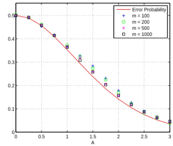
Figure 1 displays the BER of the testTσκ(A/σ)for
dif-ferent values of A and m in comparison with the
theo-retical valueQ(A/σ) of the probability of error. Table 1 gives the empirical mean and empirical Mean Square Error (MSE) of the ESE-I obtained during these experiments.
0 0.5 1 1.5 2 2.5 3 0 0.1 0.2 0.3 0.4 0.5 A Error Probability m = 100 m = 200 m = 500 m = 1000
Figure 1. BER of the testT˜σκ(A/˜σ)versus the error
prob-abilityQ(A/σ) for different values of m and A. The sig-nalsSk,k ∈ N, are independent, have their probabilities
of presence equal to1/2 and are such that Sk = AeiΦk
whereΦkis uniformly distributed in[0, 2π].
These results suggest the construction of a new estima-tor, namely the ESE-II, which basically derives from the
ESE-I.
4.3. The ESE-II
With the same notations as those used so far, letΨmbe the
random variable defined by
Ψm= 1 σ Ãm X k=1 |Yk|I(|Yk| ≤ ˜σ) ! / Ã m X k=1 I(|Yk| ≤ ˜σ) ! .
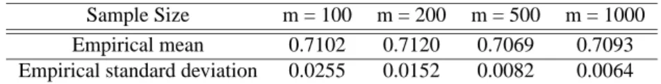
The empirical mean and standard deviation ofΨm were
computed during the experiments described in the previ-ous section. The results are those of table 2.
The empirical mean ofΨm is rather steady whenm
Sample Size m = 100 m = 200 m = 500 m = 1000 Empirical mean 1.2187 1.2289 1.2094 1.2262 Empirical MSE 0.1275 0.0995 0.0737 0.0756
Table 1. Empirical mean and empirical MSE of the ESE-I for different values of m
Sample Size m = 100 m = 200 m = 500 m = 1000 Empirical mean 0.7102 0.7120 0.7069 0.7093 Empirical standard deviation 0.0255 0.0152 0.0082 0.0064
Table 2. Empirical mean and standard deviation ofΨmfor different values ofm
random variable decreases with the sample size. Even though we only give the results obtained for m = 100, 200, 500 and 1000, the values obtained for other sample
sizes less than 1000 are quite the same. The foregoing
then suggests defining another estimateσ by settingb b σ = 1 K Ãm X k=1 |Yk|I(|Yk| ≤ ˜σ) ! / Ãm X k=1 I(|Yk| ≤ ˜σ) ! (16) where K = 0.7096 is the average value of the empirical
means ofΨmform = 100, 200, . . . , 1000. This new
esti-mateσ is called the ESE-II.b
We conducted the same type of experiments as those presented in section 4.2. The BERs obtained when the noise standard deviation is estimated by the ESE-II are
then those of figure 2. The empirical mean and empirical MSE of this estimate are given in table 3. According to these results, the ESE-II is more accurate than the ESE-I.
0 0.5 1 1.5 2 2.5 3 0 0.1 0.2 0.3 0.4 0.5 A Error Probability m = 100 m = 200 m = 500 m = 1000
Figure 2. BER of the testTbσκ(A/bσ)versus the error
prob-ability Q(A/σ) for different values of m and A. These results were obtained with the same signals and the same experimental protocol as those employed to obtain the re-sults of figure 1.
5. APPLICATION TO SPEECH ENHANCEMENT
With the same notations and under the same assumptions as those of section 1, we use the ESE-II to estimate the
noise standard deviation and adjust the Wiener filtering of the noisy speech signaly.
5.1. Standard deviation estimation via the ESE-II
We split theT available samples y[t], t = 1, 2, . . . , T , into
non-overlapping frames of N = 2q successive samples
each. As usual,q is chosen so that N Fs≈ 20ms where Fs
is the sampling frequency. LetK stand for the number of
frames such constructed. Thekth frame is then the finite
sequence of samplesy[(k−1)N
2+n], n = 0, 1, . . . , N−1.
TheN -Discrete Fourier Transform (DFT) of this frame is
then the sequenceYk,ℓ,n = 0, 1, . . . , N− 1, with Yk,ℓ= C
N −1X t=0
y[(k− 1)N + t]e−i2πℓt/N, (17)
C being some constant, usually chosen in{1, 1/N, 1/√N}.
We thus obtain the matrix[Yk,ℓ]k∈{1,...,K},ℓ∈{0,...,N −1}.
Because of the Hermitian symmetry of the DFT, we can restrict attention to half of this matrix, namely the com-plex valuesYk,ℓ,k∈ {1, . . . , K}, ℓ ∈ {0, . . . , N/2 − 1}.
Given a frame k and a bin ℓ, we should write that Yk,ℓ= Sk,ℓ+ Xk,ℓwhere, obviously,Sk,ℓandXk,ℓstand
respectively for the speech and noise time-frequency com-ponents for thekth frame and the ℓth bin. Since the frames
do not overlap, the complex random variablesXk,ℓ,k = {1, . . . , K}, ℓ ∈ {0, 1, . . . , N − 1}, are iid with Xk,ℓ ∼ Nc(0, γ2) and γ = σC√N .
Depending on the type of speech signal present during frame k, some speech time-frequency components Sk,ℓ
can be neglected in comparison with noise and other speech time-frequency components. For instance, high frequency components of voiced speech signals are often negligi-ble in comparison with noise and low-frequency compo-nents of the same speech signals; many unvoiced frica-tive speech signals have low-frequency components sig-nificantly smaller than those in high frequency and those due to noise. We model the presence and the absence of the speech time-frequency component Sk,ℓ by a discrete
random variableεk,ℓ valued in{0, 1} and write that the
observation isYk,ℓ= εk,ℓSk,ℓ+ Xk,ℓ. With respect to this
model,P ({εk,ℓ = 1}) is the probability that some speech
component be present in binℓ during the frame k. This
probability of presence may be larger than one half for low frequency components; however, for high frequency com-ponents, this probability of presence becomes less than or equal to1/2 and even relatively small.
The ESE-II is used as follows to estimate γ. We split
Sample Size m = 100 m = 200 m = 500 m = 1000 Empirical bias 1.0029 1.0103 1.0001 1.0041 Empirical MSE 0.0520 0.0302 0.0159 0.0115
Table 3. Empirical bias and empirical MSE of the ESE-II(m) for different values of m
{0, . . . , N/2 − 1}, into subsets of m observations each;
each subset is used to perform an estimate of γ via the
ESE-II; we then compute the average value of the KN/2m
estimates thus obtained to derive an estimate ofγ.
Divid-ing this average byC√N yields an estimate of σ.
In order to deal withm observations that can
reason-ably be considered as mutually independent, these obser-vations can be chosen randomly amongst theM complex
values we have. However, this randomization does not af-fect significantly the results obtained below.
5.2. The Wiener filtering
The T available samples y(t), t = 1, 2, . . . , T , are still
split into frames ofN = 2q samples each but, in contrast
with the preceding subsection, the frames overlap now by one half and the samples of each frame are weighted. De-spite these differences with the foregoing, the notations used above are kept.
The Wiener filtering of thekth frame consists in
seek-ing the complex valuesWk,ℓ, such that, for every binℓ∈ {0, 1, . . . , N − 1}, E[|Sk,ℓ− Wk,ℓYk,ℓ|2] is the least value
among all the possible quadratic meansE[|Sk,ℓ− λYk,ℓ|2]
whenλ ranges over the set of complex values. The
well-known solution to this problem is
Wk,ℓ= E[|Sk,ℓ|2]/E[|Yk,ℓ|2] = E[|Sk,ℓ|2] γ2+ E[|S k,ℓ|2] (18) sinceXk,ℓ ∼ Nc(0, γ2) and γ = σC √ N . Defining the a
priori Signal to Noise Ratio (SNR) by
ρk,ℓ= E[|Sk,ℓ|2]/γ2, (19)
equation (18) can be re-written in the form
Wk,ℓ= ρk,ℓ/(1 + ρk,ℓ). (20)
The denoised speech signal in the kth frame is then the
inverse DFT of the sequenceWk,ℓ,ℓ = 0, 1, . . . , N− 1.
The main difficulty in performing an estimate of the a priori SNR is that speech signals are not stationary. Ac-cording to the standard recursive filtering procedure origi-nally introduced in [3], we estimateWk,ℓby
f
Wk,ℓ= ˜ρk,ℓ/(1 + ˜ρk,ℓ) (21)
where
˜
ρk,ℓ= (1− α)h (ζk,ℓ− 1) + α|fWk−1,ℓYk−1,ℓ|2/γ2 (22)
can be regarded as an estimate of the a priori SNR ρk,ℓ.
In (22), h(x) = x if x ≥ 0 and h(x) = 0 otherwise, α
is some weighting factor such that0 ≤ α < 1 (we chose α = 0.98 in our experiments commented below), and
ζk,ℓ =|Yk,ℓ|2/γ2
is the so-called a posteriori SNR.
Whenσ is unknown, the value γ can be estimated by
proceeding as described in subsection 5.1. Denoting bybγ the estimate returned forγ by the ESE-II, we modify the
recursive filtering approach defined by equations (21) and (22) as follows. The coefficientsWk,ℓ are now estimated
by
c
Wk,ℓ= bρk,ℓ/(1 + bρk,ℓ), (23)
where the estimateρbk,ℓof the a priori SNR is given by b ρk,ℓ= (1− α)h ³ b ζk,ℓ− 1 ´ + α|cWk−1,ℓYk−1,ℓ|2/bγ2, (24) and bζk,ℓ = |Yk,ℓ|2/bγ2 is an estimate of ζk,ℓ. The
de-noised speech signal obtained in framek is then the inverse
DFT of the sequence cWk,ℓ,ℓ = 0, 1, . . . , N − 1. Since
it follows from section 4.3 that the estimatebγ should ap-proach significantly well the exact unknown valueγ, the
performance of the recursive procedure defined by equa-tions (23) and (24) can be expected to be close to that ob-tained by the filtering approach defined by (21) and (22).
5.3. Performance evaluation
We consider twenty sentences of the TIMIT database, down-sampled to8 kHz before adding white Gaussian noise. We
estimate the noise standard deviation as described in sec-tion 5.1 with frames ofN = 256 samples each. A frame
corresponds to32ms of noisy speech signals. For
estimat-ing the noise standard deviation, these frames do not over-lap and are not weighted. As far as the Wiener filtering is concerned, there is a50% overlap between two adjacent
frames and each frame is weighted by a Hanning window before computing the DFT.
We evaluate the quality of the filtered speech signals by means of the standard Segmental Signal to Noise Ratio (SSNR) (see [9]) and the Modified Bark Spectral Distor-tion (MBSD) (see [10]). The SSNR is the average of the SNR values on short segments. The SSNR is not relevant enough to measure the distortion of the denoised speech signals. This is the reason we use the MBSD. The MBSD proves to be highly correlated with subjective speech qual-ity assessment [10].
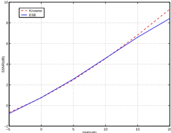
The average SNNR and MBSD obtained over the twenty sentences randomly chosen within the TIMIT database are presented in figures 3 and 4. The solid curves are the performance measurements achieved with the filtering de-fined by equations (23) and (24) where the ESE-II is used
to estimate the noise level. The dashed curves are the re-sults obtained when the filtering is achieved along equa-tions (21) and (22), that is when the noise standard devia-tion is known. Clearly, the Wiener filtering adjusted with the noise standard deviation estimate yields results that are significantly close to those obtained when the noise stan-dard deviation is known.
−5 0 5 10 15 20 −2 0 2 4 6 8 10 SNR(dB) SSNR(dB) Knownσ ESE
Figure 3. SSNR improvement for speech signals in
inde-pendent AWGN with various SNRs.
−5 0 5 10 15 20 0.02 0.025 0.03 0.035 0.04 0.045 0.05 0.055 0.06 0.065 0.07 SNR(dB) MBSD known σ ESE
Figure 4. MBSD improvement for speech signals in
inde-pendent AWGN with various SNRs.
6. CONCLUSION AND PERSPECTIVE
When signals with unknown probability distributions and priors are additively corrupted by independent WGN, the noise standard deviation can be estimated by the ESE-II.
This estimator requires no prior knowledge on the signal probability distributions, does not assume that the signals are iid or that the probabilities of presence of these sig-nals are equal. The observations should be independent; the sample size and the signal amplitudes should be large; however, these conditions are seemingly not so constrain-ing in practice.
A direct application of the ESE-II is the estimation of
the noise standard deviation when observations are speech signals in additive and independent WGN. The estimate
thus performed serves to adjust a standard Wiener filter-ing without resortfilter-ing to any VAD or subspace approaches. The SSNR and the MBSD of the denoised speech signals returned by the resulting filtering are very close to those achieved when the noise standard deviation is known.
A rather natural extension of this work is perceptual filtering. For instance, in [2], the same type of estimator is used to adjust some perceptual filtering. Our current work involves the use of the estimator proposed in the present paper to carry out perceptually motivated speech denoising in presence of white and coloured noise.
7. REFERENCES
[1] M. Abramowitz, I. Stegun, Handbook of Mathemat-ical Functions, Dover Publications, Inc., New York, Ninth printing, 1972.
[2] A. Amehraye, D. Pastor, S. Ben Jebara, On the Ap-plication of Recent Results in Statistical Decision and Estimation Theory to Perceptual Filtering of Noisy Speech Signals, ISCCSP’06, Marrakech, Morocco, 2006.
[3] Y. Ephraim and D. Malah, “Speech enhancement us-ing a minimum mean square error short-time spectral amplitude estimator”, IEEE Trans. Acoust., Speech, Signal Processing, vol. ASSP-32, 1984, pp. 1109-1121.
[4] D. Pastor, R. Gay, B. Groenenboom, A Sharp Upper-Bound for the Probability of Error of the Likeli-hood Ratio Test for Detecting Signals in White Gaus-sian Noise, IEEE Transactions on Information Theory, VOL. 48, NO. 1, pp 228-238, January 2002.
[5] D. Pastor, “Un th´eor`eme limite et un test pour la d´etection non param´etrique de signaux dans un bruit blanc gaussien de variance inconnue”, GRETSI’05, Louvain-La-Neuve, 2005.
[6] D. Pastor, “On the detection of signals with unknown distributions and priors in white gaussian noise”, Col-lection des Rapports de Recherche de l’ENST Bre-tagne, RR-2006001-SC, 2006.
[7] D. Pastor, Estimating the standard deviation of some additive white Gaussian noise on the basis of non signal-free observations, ICASSP’06, Toulouse, France, 2006.
[8] H. V. Poor, An Introduction to Signal Detection and Estimation, Springer-Verlag, 2nd Edition, 1994.
[9] S. Quackenbush, T. Barnwell, and M. Clements, “Objective Measures of Speech Quality”, Englewood Cliffs, NJ: Prentice-Hall, 1988.
[10] W. Yang, M. Dixon and R Yantorno, “Modified bark spectral distortion measure which uses noise masking threshold”, IEEE Speech coding Workshop, Pocono Manor, 1997, pp. 55-56.