HAL Id: hal-00763489
https://hal.archives-ouvertes.fr/hal-00763489
Submitted on 13 Nov 2019
HAL is a multi-disciplinary open access
archive for the deposit and dissemination of
sci-entific research documents, whether they are
pub-lished or not. The documents may come from
teaching and research institutions in France or
abroad, or from public or private research centers.
L’archive ouverte pluridisciplinaire HAL, est
destinée au dépôt et à la diffusion de documents
scientifiques de niveau recherche, publiés ou non,
émanant des établissements d’enseignement et de
recherche français ou étrangers, des laboratoires
publics ou privés.
Automated mapping of coastline from high resolution
satellite images using supervised segmentation
Anne Puissant, Sébastien Lefèvre, Simon Rougier, Jean-Philippe Malet
To cite this version:
Anne Puissant, Sébastien Lefèvre, Simon Rougier, Jean-Philippe Malet. Automated mapping of
coast-line from high resolution satellite images using supervised segmentation. Fourth international
con-ference on Geographic Object- Based Image Analysis, 2012, Rio de Janeiro, Brazil. pp.515-517.
�hal-00763489�
AUTOMATED MAPPING OF COASTLINE FROM HIGH RESOLUTION SATELLITE
IMAGES USING SUPERVISED SEGMENTATION
A. Puissant a,*, S. Lefèvre b, S. Rougier a, J.-P. Malet c
a Laboratoire Image, Ville, Environnement, CNRS ERL 7230, Université de Strasbourg, 3 rue de l’Argonne, F- 67083
Strasbourg, France
b Laboratoire de Recherche en Informatique et ses Applications de Vannes et Lorient, EA 2593 UBS, Université de
Bretagne Sud, Campus de Tohannic, Bât. ENSIbs, BP 573, 56017 Vannes Cedex, France
c Institut de Physique du Globe de Strasbourg, CNRS UMR 7516, Université de Strasbourg / EOST, 5 rue René
Descartes, F-67084 Strasbourg, France
anne.puissant[at]live-cnrs.unistra.fr sebastien.lefevre[at]univ-ubs.fr
simon.rougier[at]unistra.fr jeanphilippe.malet[at]unistra.fr
KEY WORDS: Image segmentation, Weak supervision, High resolution optical imagery, Coastline extraction ABSTRACT:
In this article, we are dealing with the problem of coastline extraction in High and Very High Resolution multispectral images. Locating precisely the coastline is a crucial task in the context of coastal resource management and planning. According to the type of coastal units (sandy beach, wetlands, dune, cliff), several definitions for the coastline has to be used. In this paper a new image segmentation method, which is not fully automated but relies on a low intervention of the expert to drive the segmentation process, is proposed. The method combines both a marker-based watershed transform (a standard image segmentation method) and a supervised pixel classification. The user inputs only consist of some spatial and spectral samples which are defined depending on the coastal environment to be monitored. The applicability of the method is tested on various types of coastal environments in France.
* corresponding author
1. INTRODUCTION
Quantitative information on coastline location is fundamental for land resource management and environmental monitoring. Land planners are interested on up-to-date information for managing human activities, for inventorying natural resources and for delineating areas exposed to hazards (Liu et al., 2007). The automatic acquisition of this information is complex, difficult and time consuming over large areas when using traditional ground survey techniques. It is also highly dependent on the morphological characteristics of the coastline (sandy beaches, rock cliffs, marshes, etc) (Puissant et al., 2008). Rapid and replicable techniques are required to monitor changes through time such as coastline retreat or aggradation.
This work proposes a new image segmentation method, which is not fully automated but relies on a low intervention of the expert to drive the segmentation process. The method combines both a marker-based watershed transform (a standard image segmentation method) and a supervised pixel classification. The user inputs only consist of some spatial and spectral samples which are defined depending on the coastal environment to be monitored. The applicability of the method is tested on various types of coastal environments in France.
2. METHODS 2.1 Marker-based watershed segmentation
The watershed transform is a very popular image segmentation
method, as it is computationally efficient and does not require any parameter. However it has also some drawbacks, such as the sensitivity to noise and above all oversegmentation (i.e., where each object-of-interest is split in many meaningless regions). To counter these limits and to increase the accuracy and relevance of the results, it is possible to consider prior knowledge. This is most often achieved by providing labelling and positions of expected regions through the definition of some markers, thus resulting in the marker-based watershed (Rivest et al., 1992). In the following, we consider the flooding paradigm (Vincent and Soille, 1991) to identify watershed lines: the image to be segmented is considered as a topographic surface f which is flooded from some initial locations defined by the set of markers M; dams are built to prevent merging water from different catchment basins in order to produce a segmentation map.
2.2 Spectral marker-based watershed segmentation
In the definition of the marker-based watershed given previously, only the spatial information brought by the set of markers is used. But when the expert defines a marker corresponding to an object-of-interest, it also provides a spectral knowledge which is involved in the segmentation process. The new segmentation scheme is thus the following.
Let us first modify the definition of the markers, considering from now a collection M = {Mi}1≤i≤c of c markers. Each
individual marker is a set of points Mi = {p}1≤p≤n, thus resulting
in either one or several connected components. These points may be characterized by various features (here only spectral characteristics are considered, but intensity, colour, or texture
features may also be used). We associate to each marker Mi a
class Ci and we apply then a given supervised (soft or fuzzy)
pixel classification, using Mi as the learning set for the class Ci.
The supervised classification procedure will return a set of probability values {wi(p)} where wi(p) represents the probability
that a pixel p would belong to the class i. From the content of a given marker Mi, we have then generated a new image wi where
high values represent pixels which most probably belong to Mi.
To fit the watershed paradigm, we define the functions fi = (1
wi) . f where pixels with a high probability wi will have their
relative input surface f lowered whereas pixels with a low probability will be kept unchanged.
The watershed algorithm (either standard or marker-based) relies on a grayscale image f. Here the supervised classification procedure results in a set of c images fi. A standard way to
combine these images is to compute a given distance (such as the Euclidean distance) as detailed in Derivaux et al. (2010). In the context of marker-based watershed segmentation, it is not necessary to merge all fi images into a single one, and we rather
consider a different image fi for each marker Mi. So the usual
algorithm (Vincent and Soille, 1991) cannot be applied directly and should be adapted to our case. More precisely, we consider here that each catchment basin, initially defined from a given marker Mi, will grow relying mainly on the surface fi built from
Mi. Several topographic surfaces fi will be involved only in case
of borderline pixels which could be assigned to different catchment basins. In other words, each pixel p is given the label of the marker Mi (or catchment basin) which reaches it first
(before the other markers or basins). This segmentation algorithm is able to consider regions of heterogeneous spectral content if markers are adequately chosen by the user and well represent the regions to be segmented. A reliable result can then be achieved by integrating both spatial and spectral information and by taking into account the user knowledge. Moreover, only a few markers are needed from the expert, thus the method can be considered as weakly supervised.
2.3 Application to coastline extraction
The experimental setup for extracting coastline from high-resolution imagery is the following. First, the expert has to provide some markers (e.g. samples) for each object-of-interest to delineate. We recall that markers are used both as spatial starting locations for the segmentation algorithm and as learning sets of the supervised fuzzy classification procedure. Thus markers have to be spectrally and spatially significant.
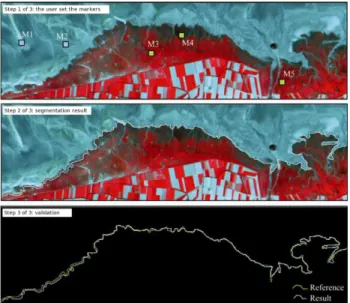
To illustrate the choice of the markers, Figure 1 shows 5 markers of similar shape (squares of 10x10 pixels) for the test site of marshy-beach at the Mount-Saint-Michel Bay characterised by a high complexity of shoreline positions. The two first markers are associated to the tidal zone: M1 for the slikke and M2 for high reflectance zones representative of shell banks. The two following markers are associated to salt marshes: M3 for those with high level of chlorophyll, dense and reached only by highest tides; M4 for those located on the pioneer line (lower density and wetter). Finally, the last marker M5 delineated a salt marsh zone.
Figure 1: Test protocol in 3 steps applied on the satellite images at the Mount-Saint-Michel Bay between 1986 and 2006, and location of the selected markers.
The computation time needed by the segmentation process is very low (a few seconds); thus it allows the user to interact with the system and to provide a more discriminative and/or complete set of markers if the result is not satisfying. Let us observe that the fuzzy supervised classification step is the actual bottleneck of the approach, and that the computation time may be decreased if the classification is performed on a sub-sampled image and membership maps are subsequently interpolated. The remaining parameters are the following: the classification algorithm in use is the five nearest neighbours (but any other classification algorithm may be used), and the gradient operator to be combined with membership maps is obtained after computing the euclidean distance of the morphological gradient applied marginally on each spectral band.
3. DATA AND STUDY SITES
For the current development and testing of the method, several high to very high resolution satellite images (Landsat, ASTER, Spot 4 & 5, Quickbird, Geoeye) of typical coastal landforms developed in sedimentary and rocky environments (sandy beach, marshy-type beach, hard-rock seacliff, soft-rock seacliff,) and typical geometry (straight line, delta, steep-wall bay) have been used (Figure 2). The regions are the sandy shoreline of Arcachon (South-West France), the marshy shoreline of the Mount Saint-Michel Bay (West France), the soft-rock cliff of Villerville (North-West France) developed in marls, the hard-rock cliff of Octeville (North-West France) developed in limestone, and the highly indentured steep-wall bay of Les Calanques near Marseille (South France).
Figure 2. Five coastal environments and their study site.
For all the study regions, several multi-resolution images (acquired in low tide periods) are available as well as reference expert mapping of the coastline that has been used for the accuracy assessment. The definition of the coastal line has to be adapted over the spatial resolution of the image and over the coastal morphology. For instance, at 30m in an urbanized and falaise coastal morphology, the coastline corresponds to the limit between sea and land. At 2m, the coastline is the foot of the falaise and the limit with the impervious surfaces. The adapted definition of the coastline retained for each spatial resolution and each type of coastal morphology is summarized in Table 1. Spatial Res. (m) Coastline definition Arcachon Sandy beach
20 - 0,4 Limit of dense vegetation Marseille Steep-wall 20 – 5 2,4 - 0,4 Limit sea/land Foot of steep-wall Limit of impervious surface St Michel Bay Salt-marshes 20 - 15 - 10 2,4 - 0,4 Limit of vegetation Octeville Hard-rock cliff 30 – 15 5 - 2,4 – 0,4 Limit of vegetation Limit of impervious surface Top of the cliff
Limit of impervious surface Vilerville
Soft-rock cliff
20 - 15 - 10 2,4 - 0,4
Limit of vegetation
Top and foot of the cliff, limit of vegetation
Table 1. Available data and selected definition of shoreline by spatial resolution.
4. RESULTS AND VALIDATION
In this short paper, the case study of the Mount-Saint-Michel-Bay is taken as example. First a qualitative evaluation has consisted in comparing the detected coastline with a ground reference digitized by a visual photo-interpretation. The quantitative assessment relies on a criterion measuring the shift (in pixels) between the reference and the extracted lines. This measure is then normalized by the length of the reference line to ensure invariant against coastline length and image size. Thus the measure may be interpreted as an average location error in each pixel.
For instance, an error of 1 means that each detected pixel is (on average) only distant of one pixel from the ground-truth (corresponding to a distance of 20m if the spatial resolution of the image is 20m). The detection error equals a half-pixel for images with a 20m spatial resolution (corresponding to a gap of 10 m between the detected line and the reference line), while for satellite images with a finer spatial resolution (10 to 15 m), the average location error is higher but still lower than one pixel. In summary, for the serie of images at the Mount-Saint-Michel-Bay, the proposed method allows to detect a line between the slikke and salt marshes with an error lower than one pixel on average. The quantitative evaluation allows to locate the detection errors. The main errors are located near tidal stream or on the pioneering line characterized by scattered salt marsh patches. Indeed, in these areas spectral responses are confused with the slikke (mudflat).
5. CONCLUSIONS AND OUTLOOK
This works presents a (semi-)automatic feature extraction for coastline from very high resolution imagery. A weakly supervised segmentation may be used to perform mapping and monitoring of changes along shorelines. This method is based on the standard marker-based watershed transform, but it also relies on spectral information brought by the user markers. In the future, we would like to consider more advanced segmentation and classification schemes to improve the method accuracy and to offer a more efficient user interaction. In particular, we are planning to involve advanced machine learning strategies (e.g., active learning, semi-supervised learning, etc.). Indeed, is has been shown recently that machine learning may greatly improves the performance of watershed-based segmentation [5].
References
Derivaux, S., Forestier, G., Wemmert, C., Lefèvre, S. 2010. Supervised segmentation using machine learning and evolutionnary computation. Pattern Recognition Letters, vol. 31, no. 15, pp. 2364–2374.
Liu, H., Sherman, D., Gu, S. 2007. Automated extraction of tidal datum referenced shoreline from airborne lidar data and accuracy assessment based on monte carlo simulation. Journal of Coastal Research, vol. 23, no. 6, pp. 1359–1369.
Puissant, A., Lefèvre, S., Weber, J. 2008. Coastline extraction in VHR imagery using mathematical morphology with spatial and spectral knowledge. In Congress of the International Society for Photogrammetry and Remote Sensing (ISPRS), Beijing, China, July 2008.
Rivest, J.F., Beucher, S., Delhomme, J. 1992. Marker-controlled segmentation: an application to electrical borehole imaging. Journal of Electronic Imaging, vol. 1, no. 2, pp. 136–142. Vincent, L., Soille, P. 1991. Watersheds in digital spaces: An efficient
algorithm based on immersion simulations. IEEE Transactions on Pattern Analysis and Machine Intelligence, vol. 13, no. 6, pp. 583–598.