Mechanical analysis and life prediction of unidirectional composites

HAL Id: tel-01562964

https://pastel.archives-ouvertes.fr/tel-01562964

HAL is a multi-disciplinary open access archive for the deposit and dissemination of sci-entific research documents, whether they are pub-lished or not. The documents may come from teaching and research institutions in France or abroad, or from public or private research centers.

L’archive ouverte pluridisciplinaire HAL, est destinée au dépôt et à la diffusion de documents scientifiques de niveau recherche, publiés ou non, émanant des établissements d’enseignement et de recherche français ou étrangers, des laboratoires publics ou privés.

Mechanical analysis and life prediction of unidirectional

composites

Elias Dib

To cite this version:

Elias Dib. Mechanical analysis and life prediction of unidirectional composites. Materials. Université Paris-Est, 2016. English. �NNT : 2016PESC1107�. �tel-01562964�

Thèse présentée pour l'obtention du grade de

Docteur de l'Université Paris-Est

Spécialité: Structures et Matériaux

Analyse numérique du comportement mécanique en

temps long des composites unidirectionnels

Numerical analysis and long-term mechanical behavior of unidirectional

composites

Elias Dib

Thèse soutenue à l’École des Ponts ParisTech le 09 décembre 2016 devant:

Rapporteurs: Alaa Chateauneuf

Jacques Lamon

Examinateurs: Fouad Kaddah

Karam Sab

Directeurs de thèse: Jean-François Caron

Wassim Raphael

Remerciement

Je souhaite remercier tout d'abord tous les membres du jury et en particulier les rapporteurs Jacques Lamon et Alaa Chateauneuf pour l’honneur qu’ils m’ont fait de lire et juger cette thèse. Vos remarques ont été précieuses et constructives.

Je tiens à remercier mon directeur de thèse, Jean-François Caron, Professeur de École des Ponts ParisTech qui m’a dirigé durant ce travail. Je lui suis reconnaissant pour ses encouragements, son enthousiasme et sa confiance.

Je souhaite adresser également mes remerciements à mon directeur de thèse, Wassim Raphael, professeur de l’École supérieure d'ingénieurs de Beyrouth pour ses conseils et ses aides durant tout ce travail de thèse.

Je voudrais également remercier Ioannis Stefanou, Enseignant – Chercheur de l’École des Ponts ParisTech pour m’avoir encadré, conseillé, surtout dans le domaine de la mécanique des matériaux ainsi que la simulation numérique et la statistique. Son aide m’a été très précieuse.

Un sincère remerciement à Fouad Kaddah Enseignant – Chercheur de l’École supérieure d'ingénieurs de Beyrouth qui m’a consacré beaucoup de son temps et qui m’a guidé, encouragé et soutenu dans mon travail.

Je remercie cordialement Monsieur Raymond Najjar pour avoir financé mon travail de thèse. Je le remercie également pour sa grande disponibilité et son humanisme.

J’adresse mes remerciements à toute l’équipe du Laboratoire Navier : les enseignants - chercheurs, les techniciens et mes collègues doctorants pour tous les échanges techniques, scientifiques et pour leur sympathie, leur accueil chaleureux pendant mon travail de thèse.

Enfin, je remercie toutes les personnes qui m’ont soutenus spécialement mon père, ma mère, mon frère et tous mes amis. Quelles soient remerciée de tout mon cœur.

Résumé

Les matériaux composites jouent un rôle de plus en plus important dans notre société et dans de très nombreux domaines (aéronautique, naval, génie civil…), grâce à leurs avantages en terme de légèreté, d’inaltérabilité et de rigidité. Cependant, ils présentent des faiblesses qui peuvent poser des problèmes au niveau de leur utilisation pour les ouvrages de génie civil. Ces faiblesses concernent notamment leur durabilité. A cause des phénomènes viscoélastiques, les propriétés mécaniques des structures en composites évoluent dans le temps. Le fluage et/ou la relaxation sont des facteurs importants qui peuvent considérablement affecter l’application des composites aux structures. Dans ce travail de doctorat, on effectue une analyse sur le comportement à court et à long terme des composites unidirectionnels renforcés par des fibres de verre/carbone. Afin d’obtenir des résultats quantitatifs sur le comportement mécanique de ces composites, différents types des sollicitations mécaniques seront considérés (ex. compression, cisaillement, tension, flexion). Les analyses sont basées sur deux modèles micromécaniques développés par l'équipe MSA. Le premier modèle est de type shear-lag viscoélastique et le deuxième utilise le logiciel éléments finis Abaqus. Ces deux modèles prennent en compte les différents micro-mécanismes de rupture comme la rupture des fibres, la décohésion des fibres/matrice et le fluage de la résine. Plusieurs analyses numériques sont faites afin de valider les différentes hypothèses de la théorie shear-lag. A partir des analyses menées, des améliorations sont apportées sur le modèle type shear-lag. Une étude comparative avec les éléments finis a permis de bien valider les résultats obtenus par la méthode shear-lag. Ayant calibré nos modèles type shear-lag et éléments finis, des simulations types court et long terme sont faites sur des composites unidirectionnels renforcées par des fibres de verre et de carbone. Les analyses sont réalisées sur plusieurs échantillons pour chaque type de fibre (Simulations de MonteCarlo). Les calculs ont montré un fluage accéléré pour les composites renforcés par des fibres de verres par rapport aux composites renforcés par des fibres de carbone.

Summary

Fiber Reinforced Plastic materials (FRP) find more and more applications in civil engineering. Besides the use of FRPs for the reinforcement of existing structures, these materials are also used quite often today for the construction of bridges and new buildings made partially or entirely of FRPs. Due to their light weight FRPs have a considerable advantage compared to conventional materials such as steel or concrete. Another advantage is that they have outstanding fatigue and durability potential and that they are in general very tolerant to environmental effects such as UV radiations, moisture, chemical attack and extreme temperature variations. However, the lack of a comprehensive, validated, and easily accessible database for the durability of fiber-reinforced polymer composites as related to civil infrastructure applications is a critical barrier to their efficient usage as main load bearing systems. The creep behavior of these materials and their failure under sustained loads remains an open research topic. This study gives a detailed analysis on the mechanical behavior of unidirectional fiber reinforced composites (UD FRP) subjected to different loading patterns (compression, shear, tension and bending). We develop two micromechanical models that allow to analyze the instantaneous and the long-term response of UD composites subjected to different load patterns. The first model is based on the shear-lag theory and the Beyerlein et al.[1998] developments while the second one is established using the Finite Element software Abaqus. A Comparative study between the two models allowed to validate the fundamental assumptions of the shear-lag theory (first model) as well as several numerical issues related to time integration and spatial discretization. The MonteCarlo method is used in order to account for the stochastic fiber strength and its impact on the ultimate tensile strength (short term) and creep (long-term). A parametric investigation on the effect of fiber type and load level/type on the short/long-term behavior of UD composites is also presented. The calculations performed showed an accelerating creep effect for fibers of inferior quality such as glass fibers compared to carbon fibers.

Content

Motivation ... 1

Chapter 1: Introduction to composite materials ... 5

1.1 Introduction ... 8

1.2 Definition of composite materials ... 9

1.3 Durability of composites ... 11 1.3.1 Moisture ... 12 1.3.2 Temperature ... 12 1.3.3 Fatigue ... 13 1.3.4 Ultraviolet ... 13 1.3.5 Alkali solutions ... 13 1.3.6 Fire ... 14 1.4 Creep of composites ... 14 1.5 Conclusion ... 29

Chapter 2: Modeling of short- and long-term behavior of FRPs under tension loads. Shear-lag vs. Finite Element models ... 30

2.1 Introduction ... 33

2.2 Theoretical basis of the shear-lag model ... 35

2.2.1 Equilibrium equations ... 36

2.2.2 Superposition technique and the auxiliary problem of an isolated fiber break . 39 2.2.3 Multiple fiber breaks simulation... 49

2.2.4 Computer simulations ... 58

2.2.5 Parameters of interest ... 63

2.2.6 Parametric analysis and validation ... 64

2.3 Finite Element Analysis ... 69

2.4.1 Ultimate tensile strength ... 71

2.4.2 Creep tests ... 81

2.5 Conclusion ... 83

Chapter 3: Statistical variability of fibers strength and its influence on creep rupture of FRPs under tension loads ... 85

3.1 Introduction ... 88

3.2 Short/Long term behavior of GFRPs/CFRPs ... 88

3.2.1 Simulation procedure ... 89

3.2.2 Ultimate tensile strength ... 90

3.2.3 Creep tests ... 92

3.3 Conclusion ... 101

Chapter 4: Creep rupture of FRPs to bending and shear loads ... 102

4.1 Introduction ... 105

4.2 Response of FRPs to bending loads ... 113

4.3 Combined shear and tension ... 116

4.4 Conclusion ... 120

Conclusion ... 121

List of Figures

Figure 1.1: Construction of a pedestrian bridge NørreAaby, Denmark 2007 extracted from FRP structures scientific and technical report 2014

Figure 1.2: Construction of Ephemeral cathedral. Peloux et al. [2015]

Figure 1.3: Classification of composites according to fibers topology

Figure 1.4: Different stages of creep

Figure 1.5: Maxwell model

Figure 1.6: Voigt model

Figure 1.7: Creep and creep recovery response of the Voigt model. Osswald n.d. [2010]

Figure 1.8: Boltzmann superposition principle. Osswald n.d. [2010]

Figure 1.9: Relaxation modulus curves for polyisobutylene and corresponding master curve at 25 0_{C, extracted from Osswald n.d. [2010]}

Figure 1.10: Shift factor as a function of temperature used to generate the master curve plotted in Figure1.9, extracted from Osswald n.d. [2010]

Figure 1.11: Tensile failure surfaces of E-glass/polyurethane composite. Abdel-Magid et al. [2003]

Figure 1.12: Smooth surface of fiber glass in the E-glass/polyurethane composite. Abdel-Magid et al. [2003]

Figure 1.13: Tensile failure surfaces of E-glass/epoxy composite. Abdel-Magid et al. [2003]

Figure 1.14: Surface of fiberglass in the E-glass/epoxy composite. Abdel-Magid et al. [2003]

Figure 1.15: Static rupture modes for GFRPs in traction and bending. Kotelnikova-Weiler [2012]

Figure 1.17: Static rupture modes for a) compression, b) combined torsion-compression, c) combined torsion-traction. Kotelnikova-Weiler [2012]

Figure 1.18: Creep rupture when combining traction with torsion. Kotelnikova-Weiler [2012]

Figure 1.19: Volume fracture for SiC fibers. Lamon et al. [1997]

Figure 1.20: Surface fracture for SiC fibers. Lamon et al. [1997]

Figure 1.21: Evolution of the deformation with time for different temperatures for GFRPs. Kouadri-boudjelthia et al. [2009]

Figure 2.1: Shear-lag model discretization

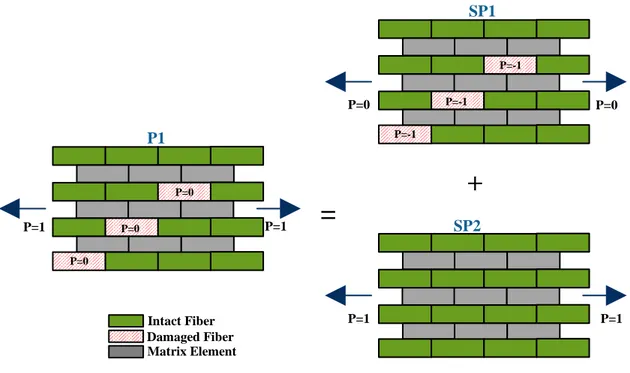
Figure 2.2: General problem P1 as a superposition of SP1 and SP2

Figure 2.3: Subproblem SP1

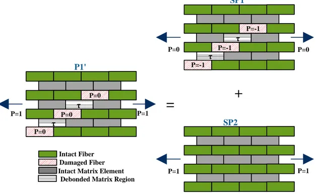
Figure 2.4: Superposition technique adopted in order to solve the problem P1'

Figure 2.5: Superposition technique adopted in order to solve the problem SP1'

Figure 2.6: Auxiliary problem A2

Figure 2.6a: Fiber/matrix debonding

Figure 2.7: Fibers strengths for a given specimen composed by 19 fibers

Figure 2.7a: Calculation algorithm (shear-lag method)

Figure 2.8: Periodicity effect

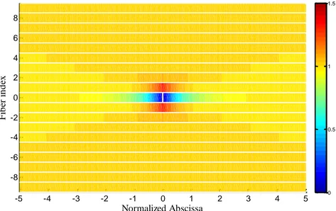
Figure 2.9: Normalized axial stress in the neighboring intact fibers due to the fiber breakage of fiber n=0. The first 8 (4+4) neighboring fibers take almost the total load (88%) of the broken fiber.

Figure 2.10: Normalized fiber axial stress (a): without periodic boundary conditions; (b): with periodic boundary conditions

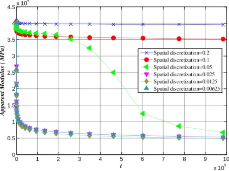
Figure 2.11: Time discretization effect. Average apparent modulus versus normalized time

Figure 2.13: Effect of fibers number. Apparent modulus versus normalized time

Figure 2.14: Length effect. Average apparent modulus versus normalized time

Figure 2.15: Finite Element model description

Figure 2.16: Calculation algorithm in the Finite Element model

Figure 2.17: Position of the imposed defect/fiber break

Figure 2.18: Normalized fiber axial stress map

Figure 2.19: Normalized fiber axial stress diagram

Figure 2.20: Normalized matrix shear stress around break site

Figure 2.21: Comparison between Finite Element and shear-lag models for the applied fiber stress versus strain curve

Figure 2.22: Comparison between Finite Element and shear-lag models for the evolution of the number of fiber breaks with the applied fiber stress

Figure 2.23: Comparison between Finite Element and shear-lag models for the fiber breaks sites at P=1900 MPa

Figure 2.24a: Normalized fiber axial stress for P=2050 MPa

Figure 2.24b: Fiber breaks sites and matrix debonded region for P=2050 MPa

Figure 2.25: Fiber stress versus strain curve (fiber/matrix debonding taken into account)

Figure 2.26: Fiber stress versus strain curve (fiber/matrix debonding neglected)

Figure 2.27: Normalized fiber stress state at P=3500 MPa (fiber/matrix debonding neglected)

Figure 2.28: Matrix shear stress state at P=3500 MPa (fiber/matrix debonding neglected)

Figure 2.29: Evolution of the number of matrix debonded elements with the applied fiber stress

Figure 2.30: Comparison between Finite Element and shear-lag models for the evolution of the apparent modulus with time

Figure 2.31: Comparison between Finite Element and shear-lag models for the evolution of the deformation with time

Figure 2.32: Comparison between Finite Element and shear-lag models for the evolution of the number of fiber breaks with time

Figure 2.33: Comparison between Finite Element and shear-lag models for the fiber break sites at the fourth time step

Figure 3.1: Probability density functions for the three types of fibers

Figure 3.2: Fibers strengths for a given specimen composed by 19 fibers

Figure 3.3: Average stress/strain curve: Finite Element method (P122 glass fibers)

Figure 3.4: Average stress/strain curve: Finite Element method (PU glass fibers)

Figure 3.5: Average stress/strain curve: Finite Element method (T300 carbon fibers)

Figure 3.6: Average apparent modulus versus time for P=0.7xPu and P=0.8xPu for P122 glass fibers

Figure 3.7: Average deformation versus time for P=0.7xPu and P=0.8xPu for P122 glass fibers

Figure 3.8: Evolution of the number of fiber breaks versus time for P=0.7xPu and P=0.8xPu for P122 glass fibers

Figure 3.9: Normalized fibers axial stress after 50 years for P122 glass fibers at P=0.8xPu

Figure 3.10: Average apparent modulus versus time for P=0.7xPu and P=0.8xPu for PU glass fibers

Figure 3.11: Average deformation versus time for P=0.7xPu and P=0.8xPu for PU glass fibers

Figure 3.12: Evolution of the number of fiber breaks versus time for P=0.7xPu and P=0.8xPu for PU glass fibers

Figure 3.13: Normalized axial stress after 50 years for PU glass fibers at P=0.8xPu

Figure 3.14: Average apparent modulus versus time for P=0.7xPu and P=0.8xPu for T300 carbon fibers

Figure 3.15: Average deformation versus time for P=0.7xPu and P=0.8xPu for T300 carbon fibers

Figure 3.16: Evolution of the number of fiber breaks versus time for P=0.7xPu and P=0.8xPu for T300 carbon fibers

Figure 3.17: Normalized axial stress after 50 years for T300 carbon fibers at P=0.8xPu

Figure 3.18: Evolution with time of the average position of rupture sites (P122/PU glass fibers)

Figure 3.19: Fitting of the deformation evolution given by shear-lag model with the Findley law for P122 glass fibers

Figure 4.1: Micro buckling failure mode

Figure 4.2: Kinking failure mode

Figure 4.3: Comparison of different models for compressive strength estimation for E-glass fibers. Naik and Kumar [1999]

Figure 4.4: Comparison of different models for compressive strength estimation for T300 carbon fibers. Naik and Kumar [1999]

Figure 4.5: Theoretical basis of the model for bending analysis

Figure 4.6: Fibers tensile strengths for a given specimen composed of 19 fibers

Figure 4.7: Number of fiber breaks versus maximum applied fiber stress for P122 glass fibers

Figure 4.8: Number of fiber breaks versus maximum applied fiber stress for T300 carbon fibers

Figure 4.9: Combining tension and shear

Figure 4.10: Stress/Strain curve for combined tension and 20% of shear stress (P122 glass fibers)

Figure 4.11: Stress/Strain curve for combined tension and 50% of shear stress (P122 glass fibers)

Figure 4.12: Stress/Strain curve for combined tension and 70% of shear stress (P122 glass fibers)

Figure 4.13: Deformation evolution with time, with and without shear stress

Figure 4.14: Apparent modulus evolution with time, with and without shear stress

Figure A.1: Model discretization for compression analysis (shear-lag method)

Figure A.2: Superposition principle

Figure A.3: Auxiliary problem A1 of a central fiber break under tension load

Figure A.4: Normalized compressive fiber axial stress calculated with the shear-lag model

Figure A.5: Normalized fibers compressive axial stress in the first intact fiber. Beyerlein et al.[2001]

List of Tables

Table 1.1: Different types of composite materials

Table 1.2: Mechanical properties of fiber materials

Table 1.3: Mechanical properties of matrix materials

Table 2.1: Average values and standard deviation values for the apparent modulus at the final time step

Table 2.2: Simulation parameters for P122 glass fibers. Zinck [2011]

Table 2.3: Comparison between overstress factors shear-lag vs. Finite Element

Table 2.4: Overstress factors with fiber/matrix debonding shear-lag vs. Finite Element

Table 3.1: Simulation parameters for T300 carbon fibers and PU glass fibers. Zinck [2011]/ Baxevanakis et al. [1998]

Table 3.2: Ultimate tensile strength for the three fiber types

Table 3.3: Stress limits of FRPs according to ACI code

Table 4.1: Compressive strength for UD composites reinforced with E-glass fibers. Naik and Kumar [1999]

Table 4.2: Compressive strength for UD composites reinforced with T300 carbon fibers. Naik and Kumar [1999]

1

2

Context:

Over the last forty years, composite materials, plastics, and ceramics have been the dominant emerging materials. The volume and number of applications of composite materials has grown steadily, penetrating and conquering new markets relentlessly. Fiberglass boats and graphite sporting goods are typical examples.

A composite material is fabricated by the combination of two or more distinct materials to form a new material with enhanced properties. For example, rocks granulates are combined with cement to make concrete. The most common composites are those made with strong fibers held together in a binder. The role of binder or matrix is to transfer the load between fibers (mostly in shear). The matrix also protects the fibers from environmental effects such as moisture, leading to corrosion resistance for instance.

Although having major advantages, composites are frequently used in civil engineering as secondary load bearing elements. This may be owed to many economical and technical reasons, but also to the lack of a comprehensive, validated, and easily accessible database for their durability and in particular for their creep behavior. Experimental results show that some of the empirical equations for creep estimation describe quite well secondary creep. However the transition from secondary to tertiary creep (rupture) is less understood, though critical for applications. Therefore studying the long term behavior of composites under various conditions remains an open, challenging topic, with important impact on their use in civil engineering.

Research goals/Originality

The importance of understanding the mechanical behavior of composites led us to develop and enhance two micromechanical models that allow assessing the short- and long-term response of unidirectional composites under any given load. The first model is based on the shear-lag theory (Cox [1952], Beyerlein et al.[1998]) taking into account the recent developments of Kotelnikova-Weiler[2012] that considered fiber/matrix debonding in the calculations, while the second one is established using the Finite Element software Abaqus. The aim of this research work was to enhance and validate the existing shear-lag numerical tool (Kotelnikova-Weiler[2012]) that simulates only tension loads and to develop a second numerical tool (based on Finite Element) that can model

3

different load patterns (such as compression, tension, bending and shear). The enhancements of the existing shear-lag model relies in the introduction of proper boundary conditions (such as periodic boundary conditions) that were neglected in the previous shear-lag models and in the verification of the main calculation assumptions such as the time step, the mesh size, the number of fibers taken into account and the length of the specimen. We note that the approach of analyzing the response (short- and long-term) of composites to tension loads obtained from the shear-lag model is different from what was presented in previous research works (Beyerlein et al.[1998]). At the matter of fact, each result obtained from the shear-lag equations (fiber stress, fiber deformation, fiber break site, fiber/matrix debonded region, number of fiber breaks, etc...) is analyzed and compared to the one obtained from the Finite Element model in order to verify its validity. Due to the stochastic behavior of the reinforcing fibers, we perform MonteCarlo simulations by considering several generated specimens in the calculations. It is to be noted that one generated specimen is not sufficient to represent the actual behavior of the composite. It is worth emphasizing that the capacity of the Finite Element model to simulate progressive fiber breakage and fiber/matrix debonding is also an important originality of the current research work since in most studies the fiber break sites and the fiber/matrix debonded regions were priory imposed (Nedele and Wisnom [1994], Blassiau et al. [2007]). The calibrated models (shear-lag and Finite Element) are also used to perform short- and long-term simulations on composites reinforced with different types of fibers (such as glass and carbon) and subjected to different loading patterns (such as compression, tension, bending and shear).

Outline of the thesis

The material covered in this current research is divided into four chapters. Its content is organized as follows:

 Chapter 1 presents a literature review on the durability of composite materials showing the influence of moisture/alkali solutions, thermal condition, creep and relaxation, fatigue, ultraviolet and fire on the life span of any structure build with composites. The creep of composites is thoroughly described in this chapter showing its different stages (primary, secondary and tertiary) and the factors that accelerate it. A literature review of the existing creep models is also presented.

4

The main role of this chapter is to highlight all the factors that triggered this research regarding the durability of composites and especially their creep behavior.

 Chapter 2 presents the shear-lag equations and the existing numerical tool which are used for the analysis of the behavior of unidirectional composites under tension loads (Beyerlein et al. [1998], Kotelnikova-Weiler[2012]). The parametric analysis that was performed herein on the shear-lag model is detailed along with the different enhancements. Furthermore, the results obtained from the enhanced shear-lag model were validated through a comparative study with the Finite Element method.

 Chapter 3 exposes the effect of the strength and statistical variability of fibers on the creep behavior of composites subjected to sustained tension loads. Different kinds of fibers, i.e. glass and carbon, were considered in the analysis and their influence on the long-term behavior of the composite and its ultimate tensile strength was explored. MonteCarlo simulations were performed using the shear-lag and the Finite Element models. The simulations showed accelerating creep effect for fibers of inferior quality, such as glass fibers compared to higher quality fibers such as carbon fibers

 Chapter 4 describes the behavior of composites under compression, bending and shearing. A literature review of the existing models used to assess the compressive strength of a unidirectional composite is presented, because unlike tension, there is no clear criterion for the fibers resistance in compression. Moreover, simulations for composites subjected to bending and shear loading are presented for different types of fibers (glass and carbon). The simulations showed accelerating creep effect under combined shear and tension loads.

 Appendix A presents a comparative study between the results obtained from the developed (shear-lag and Finite Element) numerical models and the Beyerlein et al.[2001] work on the compression behavior of unidirectional composites.

5

Chapter 1: Introduction to composite

materials

This chapter presents an overview on FRP materials highlighting the advantages that encourage their use in many domains and especially in civil engineering. It also emphasizes that the durability of these materials remains a barrier to their efficient usage as main load bearing elements in civil engineering. A description on the influence of several environmental factors on the durability of composites is briefly presented. The creep of these materials under sustained load is thoroughly described showing its different stages and its influence on the life span of any structure constructed using FRPs. The main empirical formulas that exist in the literature for creep evolution are also presented.

7

Content

1.1 Introduction ... 8

1.2 Definition of composite materials ... 9

1.3 Durability of composites ... 11 1.3.1 Moisture ... 12 1.3.2 Temperature ... 12 1.3.3 Fatigue ... 13 1.3.4 Ultraviolet ... 13 1.3.5 Alkali solutions ... 13 1.3.6 Fire ... 14 1.4 Creep of composites ... 14 1.5 Conclusion ... 29

8

1.1 Introduction

Fiber Reinforced Plastic materials (FRP) are beginning to find more and more applications in the civil engineering domain. Besides the use of FRPs for the reinforcement of existing structures, these materials are utilized quite often today for the construction of bridges and even for new buildings made entirely of composites. For instance, a 23 m long pedestrian and cycle bridge was constructed in NørreAaby, Denmark in 2007 with 100% GFRPs (Glass Fibre Reinforced Polymers or Plastics) profiles (see Figure 1.1). The Ephemeral cathedral of Creteil in France (see Figure 1.2) was built in 2013 with a GFRP gridshell structure (Peloux et al. [2015]). Another application of FRPs in civil engineering, among others, is the construction of a 41.4 m long pedestrian bridge in a Train station at Kosino, Chertanovo in Moscow in 2004. It consists of three spans - two of 15.0 m and one of 13 m length prefabricated and assembled on site. The bridge was installed in just 49 minutes.

Figure 1.1: Construction of a pedestrian bridge NørreAaby, Denmark 2007 extracted from FRP structures scientific and technical report 2014

Composites offer several advantages compared to conventional materials (such as light weight and acceptable stiffness), however their creep behavior is still not well understood. This is clearly reflected in the civil engineering design codes (ACI, Eurocomp) that impose high safety factors on structures built with composite in order to avoid creep rupture. The durability of these materials is therefore a main drawback for their use in the civil engineering domain.

9

Figure 1.2: Construction of Ephemeral cathedral. Peloux et al. [2015]

The aim of this chapter is to present a brief description on composite materials highlighting the factors that influence their durability and in particular their creep behavior. A summary on the models that exists in the literature allowing the estimation of the creep of composites is also presented. In the following chapters, the shear-lag and the Finite Element techniques used for creep predictions of composite materials will be thoroughly discussed.

1.2 Definition of composite materials

A composite material is defined as a combination of two or more materials, in general a matrix combined with reinforcement. Combining these materials gives properties superior to the properties of the individual components. In the case of a composite, the reinforcement is the fibers and is used to fortify the matrix in terms of strength and stiffness. Typical reinforcing fibers are glass, carbon and aramid. The fibers diameter usually ranges from 5 to 15 μm. The structural role of the matrix is to connect the load bearing elements (the fibers) via shear forces. The matrix also protects the fibers from abrasion and from environmental factors causing its degradation. Composites are conventionally divided into groups according to the material used for the matrix element (see to Table 1.1). In this work we are interested in analyzing the behavior of glass/carbon fiber reinforced polymers (GFRPs/CFRPs). The mechanical proprieties of some of the fiber/matrix elements are presented in Tables 1.2 and 1.3.

10

Composite type Fiber Matrix

Polymer matrix composites (PMCs)

E-glass Epoxy

S-glass Polyimide

Carbon (graphite) Polyester

Aramid (Kevlar) Thermoplastics Boron PEEK, polysulfone, etc.

Metal matrix composites (MMCs)

Boron Aluminum

Borsic Magnesium

Carbon (graphite) Titanium

Silicon carbide Cooper

Ceramic matrix composites (CMCs)

Silicon carbide Silicon carbide

Alumina Alumina

Silicon nitride Glass ceramic

Carbon matrix composites (CCCs)

Carbon Carbon

Table 1.1: Different types of composite materials

Fiber type Diameter [μm] Density [kg/m3] Young's modulus [MPa] Poisson's ratio E-Glass 16 2600 74000 0.25 S-Glass 10 2500 86000 0.2 Carbon T300 7 1750 230000 0.2 Kevlar 49 12 1450 130000 0.4 Boron 100 2600 400000 0.2

11 Matrix type Density

[kg/m3_] Young's modulus [MPa] Poisson's ratio Epoxy 1200 4500 0.4 Polyimide 1400 4000-19000 0.35 Polyester 1200 4000 0.4 PEEK 1320 3200 0.4 Polysulfone 1350 3000

Table 1.3: Mechanical properties of matrix materials

Another classification of the composite materials is based on the fibers length and distribution. Figure 1.3 shows the classification of composites according to fibers topology.

Figure 1.3: Classification of composites according to fibers topology

Although the short-term mechanical properties of these materials are well documented, the long-term mechanical behavior (durability) is less studied. In the following section, the durability of composites will be discussed.

1.3 Durability of composites

The understanding of the long-term behavior of FRPs under sustained load is vitally important in their use for structural applications. In the work of Karbhari et al. [2003] moisture/alkali solutions, thermal condition, creep and relaxation, fatigue, ultraviolet and fire were identified as crucial factors that highly influence the life span of any structure build with FRPs. The

Fiber Reinforced Composites Long Fibers Aligned oriented Unidirectional Woven Non-crimp Fabric Randomly oriented Short Fiber Bundeled dispersed oriented

12

influence of each environmental factor will be briefly discussed below and the creep behavior will be thoroughly detailed in section 1.4.

1.3.1 Moisture

Water molecules can diffuse into the network of composites to affect the mechanical properties of its constituents. The fibers are degraded by moisture and alkali due to etching and leaching actions. However, the degradation of matrices occurs due to hydrolysis, plasticization, and swelling in the presence of water. Furthermore, high moisture content weakens the interface between the fibers and the matrix which decreases the tensile properties of the composite. Shen and Springer [1977] reported that for 90 degree laminates, the ultimate tensile strength and elastic module decreased with increasing moisture content. The decrease may be as high as 50-90 percent. Bradley [1995] studied the degradation of graphite / epoxy composites due to sea water immersion. Through observation by scanning electron microscopy (SEM), they found that the measured 17% decrease in transverse tension strength was associated with the degradation of the interface, which changed the mechanism of fracture from matrix cracking to interfacial failure. The ability to predict the diffusion of water and its influences on the resin properties are necessary to predict long term behavior of composites. The uptake of moisture usually is measured by weight gain and the mechanism of water diffusion is characterized by Fick’s law. Based on Fick’s law, the study of Shen et al. [1976] presented expressions for the moisture distribution and moisture content as a function of time for one-dimensional composite materials. Many experimental data support the analytical solution determined by Shen et al. [1976] and this expression has been widely accepted to describe the water diffusion behavior in composites.

1.3.2 Temperature

The temperature effect on the mechanical properties of composites derives partly from the internal stresses introduced by the differential thermal coefficients of composite components. Such internal stresses change magnitude with temperature change, in some cases producing matrix cracking at very low temperatures. In practical applications, each polymer has its own operating temperature range. Usually a polymer has a maximum use temperature slightly below its glass transition temperature (Tg), at which the polymer transfers from rigid state to rubbery state and suffers substantial mechanical property loss. Elevated temperatures combined with humid environments have been found to magnify the problem by further reducing Tg, among other factors. The work of Marom [1989] showed that interlaminar fracture energy decreased

13

25-30% as the temperature increased from 50 to 100˚C. The interlaminar fracture surface characteristics of graphite/epoxy were also investigated in the same paper and pronounced differences were observed in the amounts of fiber/matrix separation and resin-matrix fracture with increasing temperature.

1.3.3 Fatigue

Fatigue causes extensive damage throughout the composite, leading to failure from general degradation of the material instead of a predominant single crack. There are three basic failure mechanisms in composite materials as a result of fatigue: matrix cracking, fiber breakage and interfacial debonding. Karbhari et al. [2003] in their study on GFRPs noted a reduction in the Young's modulus of the tested specimens after many cycles of loading and unloading at 45% of their ultimate tensile strength. There are many existing theories that are used to describe fatigue of composite materials. However, fatigue testing of laminates in an experimental test program is probably the best method of determining the fatigue properties of a candidate laminate.

1.3.4 Ultraviolet

The UV components of solar radiation incident on the earth surface are in the 290– 400 nm band. The energy of these UV photons is comparable to the dissociation energies of polymer covalent bonds, which are typically 290–460 kJ/mol. Thus, UV photons absorbed by polymers result in photo-oxidative reactions that alter the chemical structure resulting in material deterioration. In literature (Brook [2002] for instance), there are few investigations that focus on the effects of UV radiation on the degradation of mechanical properties of FRPs. Brook [2002] reported that for relatively short periods of exposure, only changes in surface morphology are observed. However, for extended exposure to UV radiation, matrix properties can suffer severe deterioration, e.g. interlaminar shear strength and flexural strength and flexural stiffness can all decrease. The fiber properties, such as tensile modulus and tensile strength, are usually not affected significantly, especially for carbon fiber-reinforced materials.

1.3.5 Alkali solutions

The effect of alkaline and acid solutions on the FRPs mechanical properties is widely analyzed by many researchers. Even though, the studies that exist in the literature are not sufficient to establish a full knowledge of this subject. Rakin et al.[2011] studied the effect of alkaline and acid solutions on the tensile properties of glass-polyester composites. They concluded that the alkaline solution decreases the tensile properties (ultimate tensile strength and Young's modulus) and this tendency increases with the pH value. According to the study of Kawada et

14

al. [2001], stress-corrosion cracking in GFRPs occurs as a result of a combination of loads and exposure to a corrosive environment. Sharp cracks initiate and propagate through the material as a direct consequence of the weakening of the glass fibers by the acid. The strength of the fibre reduces dramatically as a result of diffusion of acid and chemical attack which causes a highly planar fracture with a much reduced failure stress.

1.3.6 Fire

Heat causes the polymer to melt which induces degradation of mechanical properties of the composite. Polymer transforms from solid phase to rubbery or semi-liquid phase once the matrix resin temperature goes above the glass transition temperature Tg. Tg is often well below the decomposition temperature of the polymer, which is the temperature at which enough heat energy has entered into the polymer to cause bonds to begin to break and the polymer to fragment. This leads to the loss of the mechanical properties of the composite as the matrix resin vaporizes. One notable example for the influence of heat on composites is the Norwegian minesweeper Orkla, which was an all composite vessel that caught fire and rapidly sank in November 2002.

1.4 Creep of composites

Another crucial factor that highly influences composites durability is creep. By definition, the creep is the ability of a material to deform under sustained load (see Figure 1.4). Its initial stress-strain behavior can be considered as linear elastic. Under sustained loading the material creeps with a steady strain-rate until tertiary creep takes place. Tertiary creep is related to an increase in deformation rate under, again, constant loading, and eventually failure. The behavior of the glass or carbon fibers is brittle and cannot justify rate effects at the observed time scale of transition from secondary to tertiary creep. However, the viscoelastic behavior of the matrix elements can. Many theoretical and empirical relations exist in the literature allowing the calculation of the evolution with time of the deformation of a material under sustained load. We will briefly cite below some of the models that exists in the literature for creep calculations.

15 Time t S tr ai n, ε Primary Secondary Tertiary Initial Strain σ =Constant T =Constant σ Time t S te ss σ Fracture

Figure 1.4: Different stages of creep Creep Models

One of the first models that were used for creep evaluation is the Maxwell model. The Maxwell model can be represented by a spring and a viscous damper connected in series (see Figure 1.5). Maxwell calculated the elastic component of the strain that occurs instantaneously, corresponding to the spring, and relaxes immediately upon release of the stress and allows the estimation of a second component of the strain which is a viscous component that grows with time as long as the stress is applied (viscous damper effect). The model predicts that stress decays exponentially with time, which is accurate for most polymers.

Figure 1.5: Maxwell model

We present briefly the equations of the Maxwell model:

If we consider the Hook's law for the spring:

𝜎 = 𝐸𝜀 (1.1)

where 𝜎 is the applied stress, 𝜀 is the specimen deformation and 𝐸 is the elastic stiffness of the spring.

16 𝜎 = 𝜂𝑑𝜀

𝑑𝑡 (1.2)

where 𝜂 is the viscosity modulus and 𝑡 is the time.

Combining equations (1.1) and (1.2) leads to:

𝑑𝜀 𝑑𝑡= 1 𝐸 𝑑𝜎 𝑑𝑡 + 𝜎 𝜂 (1.3)

The Maxwell model for creep or constant-stress conditions postulates that strain rate will increase linearly with time. However, polymers for the most part show a strain rate decreasing with time.

Another model for creep predicting was presented by Voigt. The model of Voigt consists of a spring and a viscous damper connected in parallel (see Figure 1.6). The spring models the elastic response while the dashpot models the viscous/time dependent response to the applied load.

Figure 1.6: Voigt model

The governing equation for the Voigt model is:

𝜎 = 𝐸𝜀 + 𝜂𝑑𝜀

𝑑𝑡 (1.4)

where 𝜂 and 𝐸 are the viscosity and Young’s modulus respectively. Using the above equation, the strain in a creep test (constant stress) in the Voigt model can be solved with:

𝜀 =𝜎

𝐸(1 − 𝑒𝑥𝑝

−𝑡/𝜏_{) (1.5)}

17

Figure 1.7 shows the creep and recovery curve for the Voigt model.

Figure 1.7: Creep and creep recovery response of the Voigt model. Osswald n.d. [2010]

The Voigt model predicts creep more realistically than the Maxwell model. However, the Voigt model is not good at describing the relaxation behavior after the stress/load is removed.

Superposition techniques are also introduced in the literature in order to model creep. The Boltzmann superposition technique is one of the methods. It describes the response of a material to different loading histories. The Boltzmann superposition technique (see Figure 1.8) is based on the hypothesis that the response of the material to a given load is independent of the response of the material to any load which is already applied on the material. Therefore at a given temperature, the deformation of the material is proportional to the applied stress. The total strain may be expressed by equations 1.7 and 1.8.

𝜀(𝑡) = 𝐷(𝑡 − 𝜏1) + 𝐷(𝑡 − 𝜏2)(𝜎2− 𝜎1) + ⋯ + 𝐷(𝑡 − 𝜏𝑖)(𝜎𝑖 − 𝜎𝑖−1) (1.7) Or 𝜀(𝑡) = ∫ 𝐷(𝑡 − 𝜏)𝑑𝜎(𝑡) (1.8) 𝑡 0 where 𝐷(𝑡) = 1 𝐸(𝑡) (1.9)

where 𝐷(𝑡) is the creep compliance function which is a characteristic of the polymer at a given temperature. Figure 1.8 shows the response of a material to applied stress according to the Boltzmann superposition technique.

18

Figure 1.8: Boltzmann superposition principle. Osswald n.d. [2010]

At a given time 𝑡₁, the strain 𝜀₁induced by an applied stress 𝜎₁ is:

𝜀₁(𝑡) = 𝜎₁𝐷(𝑡) (1.10) According to linear viscoelasticity, the compliance 𝐷(𝑡) is independent of the stress. Therefore if a stress increment 𝜎₂− 𝜎₁ is applied at a time 𝜏₂, the strain increase due to the stress increment can be expressed with equation 1.11:

𝜀₂(𝑡) = 𝐷(𝑡 − 𝜏₂)(𝜎₂− 𝜎₁) (1.11) Likewise the strain increase due to 𝜎₃− 𝜎₂can be written with equation 1.12:

𝜀₃(𝑡) = 𝐷(𝑡 − 𝜏₃)(𝜎₃− 𝜎₂) (1.12) A generalized form of the Boltzmann superposition technique can be written with equation 1.13: 𝜀(𝑡) = 𝐷0𝜎 + ∫ ∆𝐷(𝑡 − 𝜏) 𝑑𝜎 𝑑𝜏 𝑡 0 𝑑𝜏 (1.13)

In a similar way the relaxation of the material can be determined with equation 1.14:

𝜎(𝑡) = 𝐸₀𝜀 + ∫ ∆𝐸(𝑡 − 𝜏)𝑑𝜀 𝑑𝜏 𝑡

0

𝑑𝜏 (1.14)

Another superposition technique which is well used is the time temperature superposition principle (TTSP). It describes the equivalence of time and temperature. The time temperature superposition technique is used in order to obtain the creep behavior of a material at a given temperature using creep curves at different temperature levels which can be shifted along the

19

time axis. Figure 1.9 shows an example of relaxation modulus curves for time temperature superposition extracted from Osswald.n.d.[2010]. Relaxation curves made at different temperatures are superposed by horizontal shifts along a logarithmic time scale to give a single master curve covering a large range of times.

Figure 1.9: Relaxation modulus curves for polyisobutylene and corresponding master curve at 25 0_{C, extracted from Osswald n.d. [2010]}

The amount that each curve was shifted can be plotted with respect to the temperature difference taken from the reference temperature (see Figure 1.10).

Figure 1.10: Shift factor as a function of temperature used to generate the master curve plotted in Figure 1.9, extracted from Osswald n.d.[2010]

Williams, Landel and Ferry (Ferry [1955]) established the WLF equation that determines the shifting factors 𝑎_𝑇.

𝑎_𝑇 = − 𝐶1(𝑇 − 𝑇𝑟𝑒𝑓)

𝐶₂+ (𝑇 − 𝑇_𝑟𝑒𝑓) (1.15) where 𝐶₁ and 𝐶₂ are material dependent constants.

20

It has been shown that for most polymers 𝐶₁ = 17.44 and 𝐶₂ = 51.6 if the reference temperature 𝑇𝑟𝑒𝑓 is chosen as glass transition temperature. Often, the WLF equation must be adjusted until it fits the experimental data. Master curves of stress relaxation tests are important because the polymer’s behavior can be traced over much longer periods than those that can be determined experimentally.

In summary, the application of the TTSP typically involves the following steps:

 Experimental determination of frequency-dependent curves of isothermal viscoelastic mechanical properties at several temperatures and for a small range of frequencies.

 Computation of a translation factor to correlate these properties for the temperature and frequency range.

 Experimental determination of a master curve showing the effect of frequency for a wide range of frequencies.

 Application of the translation factor to determine temperature-dependent module over the whole range of frequencies in the master curve.

The application of the time temperature supperposition principle is proven to be adequate by multiple studies. Alwis and Burgoyne [2006] demonstrated that creep curves for composites reinforced with aramid fibers can be obtained by using the TTSP. The authors discussed the methods to be used in order to obtain smooth master curves and confirmed the validity of the resulting curves and the corresponding stress-rupture lifetime. Miyano et al.[2008] validated in their study the TTSP and they also demonstrated the applicability of their accelerated testing methodology (ATM). The ATM method is based on the time temperature superposition technique. Using this method the authors predicted the long-term fatigue life of polymer matrix composites.

In the studies cited above, among others, the Boltzmann superposition technique as well as of the TTSP are generally used only in the case of linear viscoelasticity. Several models have been developed in order to describe the nonlinear viscoelasticity. In fact, Findley [1956] developed a nonlinear form of a power law in order to predict the creep behavior of laminated clothed reinforced plastics. At a later stage Findley and Peterson [1958] showed that the existing model accurately predicted the creep behavior of four types of plastic materials for 10 years of experimental data. The basic form of the Findley power law is:

21 where 𝜀0 = 𝜀0′sinh 𝜎 𝜎𝜀 (1.17) 𝑚 = 𝑚′sinh 𝜎 𝜎𝑚 (1.18) 𝜀₀′, 𝜎_𝜀, 𝑚′_{, 𝜎}

𝑚 and 𝑛 are all material dependant parameters which may be functions of temperature, absorbed moisture content, etc..., but are assumed not to be functions of time or the applied stress level. Boller [1965] proposed a simple method for evaluating the power law parameters. A more accurate least square approach was introduced at later stage in order to properly evaluate these parameters. Multiple applications and verifications to the power law proposed by Findley exist in the literature. Dillard et al. [1987] study led to the conclusion that the nonlinear procedure proposed by Findley could be used to accurately fit the experimental data of creep test for T300/934 graphite/epoxy composites. Furthermore, Yen et al.[1990] validated the Findley power law expression in his study on chopped fiber composites. Bank and Mosallam [1992] analyzed the short and the long term behavior of a frame structure build with pultruded beams and columns. Creep test were performed at sustained flexural load. The authors reported good agreement between the experimental data and the results obtained using the Findley law.

Schapery's [1969] also contributed in the development of models for nonlinear viscoelasticity. Schapery's [1969] model is based on irreversible thermodynamics. For uniaxiale loading under isothermal conditions, this approach takes the form:

𝜀(𝑡) = 𝑔₀𝐷₀𝜎 + 𝑔₁∫ ∆𝐷(𝜓 − 𝜓′₎𝑑𝑔2𝜎 𝑑𝜏 𝑡

0

𝑑𝜏 (1.19)

where 𝐷₀ and ∆𝐷(𝜓) are the initial and the transient component of the linear viscoelastic creep compliance, respectively. 𝜓 = 𝜓(𝑡) = ∫ 𝑑𝑡′ 𝑎𝜎 𝑡 0 (1.20) 𝜓′ = 𝜓′(𝜏) = ∫ 𝑑𝑡 ′ 𝑎_𝜎 𝜏 0 (1.21)

22

The parameter 𝑔₀ is related to the nonlinear instantaneous compliance, 𝑔₁ is associated with the nonlinear transient compliance, and 𝑔2 is related to the loading rate effect on nonlinear response. The parameter 𝑎_𝜎 is the horizontal shift factor for stress and it is used in the same manner as the temperature shift factor 𝑎_𝑇. Lou and Schapery [1971] extended the Schapery's [1969] integral model to characterize the nonlinear time-dependent behavior of glass fiber reinforced epoxy. The Schapery single integral approach has been shown to be accurate and adaptable by many studies (Dillard et al. [1987], among others ).

Experimental work was also performed in the aim of understanding the failure mechanism of composites subjected to sustained loads. For instance, Abdel-Magid et al. [2003] investigated the creep rupture of two systems of E-glass reinforced polymer composites (E-glass/polyurethane and E-glass/epoxy) subjected to sustained bending load. The two composite systems showed similar short-term mechanical behaviors, however their long term creep behaviors were quite different. The E-glass/polyurethane system exhibited tertiary creep leading to rupture within a few hours when subjected to about 60% of its flexural strength while the E-glass/epoxy endured months of loading at 60% of its flexural strength before rupture. Scanning electron microscopy (SEM) was used to study the failure surface of the specimens. Figure 1.11 shows SEM photomicrograph of the tensile failure surface of E-glass/polyurethane composites. The fibers in Figure 1.11 are shown pulled out of the resin before failure. The fibers on the tension failure surface of this material seem clean and smooth with no traces of resin on their surface.

Figure 1.11: Tensile failure surfaces of E-glass/polyurethane composite. Abdel-Magid et al. [2003]

23

A closer look on the fiber surface (see Figure 1.12) reveals the absence of matrix around the fiber. This indicates poor interfacial bonding between the polyurethane and the E-glass fibers.

Figure 1.12: Smooth surface of fiber glass in the E-glass/polyurethane composite. Abdel-Magid et al. [2003]

Moreover, Figure 1.13 shows that the matrix in the E-glass/epoxy composite surrounds the fibers, indicating better interfacial bond between fiber and matrix.

Figure 1.13: Tensile failure surfaces of E-glass/epoxy composite. Abdel-Magid et al. [2003]

This is further indicated by the rough surface of the fiberglass shown in the enlarged image in Figure 1.14.

24

Figure 1.14: Surface of fiberglass in the E-glass/epoxy composite. Abdel-Magid et al. [2003]

The authors reported that the interfacial bonding is most likely responsible for the difference in the creep-rupture behavior of the two materials.

Furthermore, the experimental work performed by Kotelnikova-Weiler[2012] during her PhD thesis, highlighted the role of the matrix in the creep rupture of composites. Creep tests for different FRP specimens were performed by Kotelnikova-Weiler[2012] under various types of loading (bending, traction, compression and torsion) and at various load levels. At first, the static strength of the specimens under tension and bending loads was estimated and the failure modes of the specimens to bending and traction were presented (see Figure 1.15).

25

Figure 1.15: Static rupture modes for GFRPs in traction and bending. Kotelnikova-Weiler [2012]

When creep tests were performed, Kotelnikova-Weiler[2012] reported that the GFRP specimens attained creep rupture at load levels lower than their initial strength (see Figure 1.16).

Figure 1.16: Creep rupture under bending load for GFRPs. Kotelnikova-Weiler [2012]

In order to stimulate the matrix element, Kotelnikova-Weiler[2012] combined torsion to the tension or compression loads. Instantaneous failure modes due to pure compression, to combined compression and torsion and combined traction and torsion were also presented by Kotelnikova-Weiler[2012] (see Figure 1.17).

26

Figure 1.17: Static rupture modes for a) compression, b) combined torsion-compression, c) combined torsion-traction. Kotelnikova-Weiler [2012]

The author reported that when pure compression load was applied to the specimen, kink band mode was observed (Figure 1.17a). The application of a torsional load combined with the compression induced an instantaneous crush of the sample leaving an almost clean surface (Figure 1.17b). Longitudinal cracking was observed for specimens where torsion and traction were combined (Figure 1.17c). In parallel to short term tests, creep tests were also performed with the combined loads configuration. Combined tension and torsion loads were applied to the specimens at different loading levels. Kotelnikova-Weiler[2012] proclaimed that; when torsion was combined with tension, the creep rupture of the specimens was accelerated (see Figure 1.18 for the creep rupture mode under combined tension and torsion).

Figure 1.18: Creep rupture when combining traction with torsion. Kotelnikova-Weiler [2012]

The experimental work of Lamon et al. [1997] showed that the failure of composites reinforced with SiC fibers is related to the presence of two partially concurrent flaw populations at the fibers level (extrinsic, intrinsic). The extrinsic flaws are located in the surface and the intrinsic flaws are located both in the surface and in the volume of SiC fibers. SEM examination of

27

fracture surfaces revealed the presence of fracture-inducing flaws located in the surface or in the interior of fibers (see Figures 1.19 and 1.20).

Figure 1.19: Volume fracture for SiC fibers. Lamon et al. [1997]

Surface-located fracture origins dominated failure at the low strengths or strains, whereas volume-located fracture origins were essentially identified in those fibers that failed at higher stresses or strains. It is worth mentioning that the Weibull's [1951] model is the most widely used for the description of the statistical distribution of failure strengths of fibers under uniaxiale stress states. This model will be thoroughly explained in the following chapters.

Figure 1.20: Surface fracture for SiC fibers. Lamon et al. [1997]

In addition to the role of the constituents (fibers, matrix, fiber/matrix interface), other factors may accelerate the creep of composites such as temperature and solicitation time. Figure 1.21 for example shows the evolution of the deformation with time curves at different temperatures

28

for GFRP specimens according to Kouadri-boudjelthia et al. [2009]. Figure 1.21 shows that the creep rupture is accelerated with the increase of temperature.

Figure 1.21: Evolution of the deformation with time for different temperatures for GFRPs. Kouadri-boudjelthia et al. [2009]

Based on the role played by each of the composite constituents (fiber, matrix and fiber/matrix interface) in the creep rupture phenomena, Cox [1952] has introduced a method called shear-lag that allows estimating the stresses and strains in the microstructure of a unidirectional composite subjected to tension load. The author proposed an analytical model for determining the stresses around a single fiber break in a linear elastic matrix. Several enhancements were performed on the Cox's model by many researchers (Hedgepeth [1961], Hedgepeth and Dyke [1967], Lagoudas et al. [1989], Ochiai [1991], Sastry and Phoenix [1993], among others). Their work will be thoroughly detailed in chapter 2. An alternative approach to shear-lag theory for creep modeling of composites was the Finite Element method. Several researcher used this technique to compute the time dependent behavior of UD composites (Nedele and Wisnom [1994], Blassiau et al. [2007],Thionnet and Renard[1998], among others). A detailed literature review on the use of the Finite Element method for analyzing the creep of composite will also be presented in chapter 2. In this research work, we take benefit from the shear-lag and Finite Element modeling techniques to develop numerical models that allow us to analyze the behavior of unidirectional composite subjected to different loading patterns such as tension, compression, bending and shear. The analysis will be thoroughly detailed in chapters 2, 3 and 4.

29

1.5 Conclusion

The durability of composite materials was thoroughly discussed in this chapter. The effect of moisture/alkali solutions, thermal condition, creep and relaxation, fatigue, ultraviolet and fire on the life span of any structure constructed with FRPs was also highlighted. A literature review on the theoretical models that exists for creep prediction was also exposed. The advantage and the disadvantage of each model were explained showing that the creep of composites is still an open research topic. Several experimental works that led to identifying the influence of each of the composite constituents (fibers, matrix, and fiber/matrix interface) on creep rupture were presented. The aim of the literature review on creep was to understand its different stages and to know all the factors that accelerate it. All the above led us to choosing modeling techniques that accurately predicts the creep of composites. The shear-lag method based on the development of Beyerlein et al. [1998] and enhanced during the thesis Kotelnikova-Weiler[2012] was chosen to do such task. Since the proposed technique can model fiber breakage, fiber/matrix debonding and matrix viscoelasticity. However, several simplifications/assumptions were identified in the existing shear-lag model. The periodic boundary conditions for instance were neglected and representative volume element parameters were not properly justified. The enhancements and validation of the existing shear-lag model are thoroughly detailed in the following chapter.

30

Chapter 2: Modeling of short- and

long-term behavior of FRPs under tension loads.

Shear-lag vs. Finite Element models

In this chapter the mechanical behavior of unidirectional composites subjected to sustained tension load is analyzed. In order to perform this task, two modeling techniques are used. The first technique is based on the shear-lag theory (Beyerlein et al.[1998], Kotelnikova-Weiler [2012]). The second one is based on the Finite Element method. The shear-lag equations along with all the assumptions that were considered in the calculations are detailed in this chapter. A parametric analysis of the shear-lag model is also presented together with some enhancements to the existing technique. A comparative study between the developed shear-lag and Finite Element models is then presented.

32

Content

2.1 Introduction ... 33 2.2 Theoretical basis of the shear-lag model ... 35 2.2.1 Equilibrium equations ... 36 2.2.2 Superposition technique and the auxiliary problem of an isolated fiber break . 39 2.2.3 Multiple fiber breaks simulation... 49 2.2.4 Computer simulations ... 58 2.2.5 Parameters of interest ... 63 2.2.6 Parametric analysis and validation ... 64 2.3 Finite Element Analysis ... 69 2.4 Comparison of shear-lag and Finite Element modeling results ... 71 2.4.1 Ultimate tensile strength ... 71 2.4.2 Creep tests ... 81 2.5 Conclusion ... 83

33

2.1 Introduction

As previously discussed in chapter 1, composites are subjected to degradation problems when exposed to heat, light, weathering, high energy radiation, chemicals, and microorganism. In addition to these environmental factors, and as consequence to the viscoelastic properties of the matrix part, composites deform with time when subjected to constant stress. The deformation of these materials with time (named creep) may lead to rupture. The creep of composite is divided into three stages. The primary region is the early stage of loading when the strain rate of the material decreases with time. Then it reaches a steady state which is called the secondary creep stage followed by a rapid increase (tertiary stage) and fracture. Tertiary creep or creep rupture can occur at load levels lower than the ultimate strength of the composites. Therefore it is of high interest to properly evaluate the creep of composites under different loading patterns. In this part of the thesis, we are interested in analyzing the behavior of composite under sustained tension load.

In order to properly understand the composites behavior under tension load, one must understand the sequence of its failure mechanism. At the matter of fact, failure of unidirectional composites occurs after accumulation of many fiber breaks (cluster formation of broken fibers), which are finally localized at a fracture plane perpendicular to the direction of the principle tensile stress. The matrix role is to connect the fibers and to transfer the shear forces. The fibers are the main load bearing elements. However, the viscoelastic behavior of the matrix element is responsible for the creep behavior of the composite at the macro scale. Based on these facts, Cox [1952] has introduced a method called shear-lag that allows to estimate the stresses and strains in the microstructure of a unidirectional composite subjected to tension load. The author proposed an analytical model for determining the stresses around a single fiber break in a linear elastic matrix. However, Cox neglected the effect of the surrounding fibers and the effect of the matrix stiffness in parallel to the fiber direction. Hedgepeth [1961] removed this limitation and generalized Cox's model in two dimensions (2D shear-lag model). Hedgepeth numerical model allows to estimate the overstress factors induced by a single fiber break to its neighboring intact fibers in a two dimensional unidirectional composite. The author demonstrated that the broken fiber sheds its load to nearby intact fibers which causes stress concentration in the fibers near the break site. Later Hedgepeth and Dyke [1967] extended the above work in three dimensions, by considering both square and hexagonal spatial configurations for the fibers. The overstress factors induced by fiber breaks were estimated based on the nearest neighbor approximation, i.e. only the immediate fibers next to the broken one were affected by the break. The overstress

34

factors calculated by Hedgepeth and Dyke [1967] in their 3D analysis were smaller than the ones calculated when 2D configuration was considered (Hedgepeth [1961]). This fact proves that 2D calculations are conservative and can be considered for applications. Moreover, Lagoudas et al. [1989] introduced the viscoelastic behavior of the matrix to the modeling process. The authors calculated the evolution with time of fiber and matrix stresses around an arbitrary array of fiber breaks in a unidirectional composite subjected to tension load. Ochiai [1991] completed these models by taking into account the matrix stiffness parallel to the direction of the fibers.

In the aforementioned shear-lag models, the fiber breaks were a priori imposed as defects in the composite material and new fiber breaks were not possible. Beyerlein et al.[1998] developed a computational technique, called viscous break interaction, allowing to determine the evolution with time of fiber and matrix stresses around an arbitrary array of fiber breaks in a unidirectional composite. In their model, new fiber breaks are allowed. However, Beyerlein et al.[1998] neglected the effect of fiber/matrix debonding when viscoelastic matrix behavior is considered. This phenomena was taken into account by Kotelnikova-Weiler[2012] by considering a viscous behavior for the matrix element combined with fiber/matrix debonding. The aforementioned model that was developed in the work of Kotelnikova-Weiler[2012] is presented, enhanced and validated in this chapter. In particular, an extensive parametric study regarding the time integration and the spatial discretization is performed. This allowed to investigate the convergence of the numerical results of the shear-lag theory. The existing numerical model was also extended in order to take into account periodic boundary conditions that enable the derivation of the effective properties of the material.

In the aim of validating the shear-lag model, a Finite Element model was also developed in this thesis. It is worth mentioning that the Finite Element method was used by several researchers (Nedele and Wisnom [1994], Thionnet and Renard[1998], Xia, Chen, and Ellyin [2000]) as alternative to shear-lag theory for studying the creep of composites. However, these Finite Element models do not account for the graduate breakage of the fibers and the evolution of the mechanical behavior of UD composites in time (creep). Moreover, they do not perform stochastic analyses (MonteCarlo) which is important for determining the expected ultimate strength and time behavior of the material.