Transactions in GIS. 2018;1–14. wileyonlinelibrary.com/journal/tgis
|
11 | INTRODUCTION AND PREVIOUS WORK
Land change (LC) science seeks to understand the dynamics of land cover and land use change (Turner, Lambin, & Reenberg, 2007). However, land cover is a distinct concept from land use. Land cover is the physical material that covers a specific land of the Earth, whereas land use shows how people use the land (Fisher, Comber, & Wadsworth, 2005). For example, the grass is a land cover which can be found in many land uses such as urban parks and pastures.
R E S E A R C H A R T I C L E
Benefits of a multiple‐solution approach in land
change models
Ahmed Mustafa
1| Amr Ebaid
2| Jacques Teller
1This is an open access article under the terms of the Creative Commons Attribution License, which permits use, distribution and reproduction in any medium, provided the original work is properly cited.
© 2018 The Authors. Transactions in GIS published by John Wiley & Sons Ltd
1LEMA, Urban and Environmental Engineering
Department, Liège University, Liege, Belgium
2Department of Computer Science, Purdue
University, West Lafayette, Indiana, USA Correspondence
Ahmed Mustafa, LEMA, Urban and
Environmental Engineering Department, Liège University, Allée de la Découverte 9, Quartier Polytech 1, 4000 Liège, Belgium.
Email: [email protected]
Abstract
Land change (LC) models are dedicated to a better under‐ standing of land use and land cover dynamics. A funda‐ mental aspect of those models lies in the calibration of spatial parameters underlying such dynamics. Although there are many studies on the calibration of LC models, current efforts have a common goal of seeking to find a single global optimum solution, even though land change dynamics may be inherently heterogeneous throughout a given space. This article presents a calibration approach for finding multiple optimal solutions. A crowding niching genetic algorithm (CNGA) is incorporated into a cellular au‐ tomata LC model. The model is applied to simulate urban expansion in Wallonia (Belgium) as a case study. Our find‐ ings demonstrate the ability of the model to locate multiple solutions simultaneously. In addition, the CNGA performs better than the standard genetic algorithm—besides, the CNGA helps to better understand the properties of land change dynamics within a given landscape.
During the last two decades, a wide range of LC models have been developed and applied to understand and/or predict transitions in land change. The assessment of different models depends on the quality of their outcomes, and therefore model calibration is a critical step in the construction of the model (van Vliet et al., 2016). Several methods have been proposed in the literature to calibrate spatial LC models, including a visual test (e.g., Clarke, Hoppen, & Gaydos, 1997; Ward, Murray, & Phinn, 2000), multi‐criteria evaluation (e.g., Mahiny & Clarke, 2012), reusing param‐ eters from other studies (e.g., Mustafa, Saadi, Cools, & Teller, 2015), statistical analysis (e.g., García, Santé, Boullón, & Crecente, 2013), machine learning (e.g., Mileva, Suzana, Miloš, & Branislav, 2015), artificial neural networks (e.g., Basse, Omrani, Charif, Gerber, & Bódis, 2014; Pijanowski et al., 2014), and search algorithms for optimization such as genetic algorithms (e.g., Mustafa, Heppenstall et al., 2018), particle swarm optimization (e.g., Feng, Liu, Tong, Liu, & Deng, 2011), and a combination of various methods (e.g., Mustafa, Cools, Saadi, & Teller, 2017). Although there is no standard calibration method, statistical analysis is one of the most frequently applied calibration approaches (van Vliet et al., 2016). However, a number of studies compared the performance of statistical analysis‐based calibration with other methods, including machine learning methods (e.g., support vector machines; Mustafa, Rienow, Saadi, Cools, & Teller, 2018) and evolutionary population‐based search methods (e.g., particle swarm optimization; Feng et al., 2011). Those studies demonstrated that machine learning and evolutionary population‐based search methods outperformed statistical calibration methods.
Genetic algorithms (GAs) are powerful optimization methods, proposed by Holland in the 1960 and 1970s (Holland, 1975). They have already been successfully applied to many LC models (e.g., Al‐Ahmadi, See, Heppenstall, & Hogg, 2009; García et al., 2013; Liu et al., 2015). Pareto front methods are often integrated with GAs to illustrate the trade‐off among conflicting optimization objectives, which assists in optimizing the allocation of different, conflicting, land uses simultaneously (Mustafa, Heppenstall et al., 2018). A typical GA consists of a genetic repre‐ sentation of the problem space, an objective function to evaluate each candidate solution, and selection, cross‐ over, and mutation operators. A GA starts by generating a first generation of individuals, often randomly. Each generation has a set of individuals (population) that are evaluated through an objective function. For each new generation, the GA selects a portion of the existing population to act as parents to breed a new generation using a crossover operator in which two parents are combined to create a new child. Each child is altered by a mutation operator that adds a small random number to each gene. The GA hence tries to maintain genetic diversity from one generation to the next. Owing to the use of a population, a GA can theoretically find multiple local optimal solutions. However, most standard GAs tend to prematurely converge to one optimal solution, because they have difficulty maintaining population diversity during evolution (Črepinšek, Liu, & Mernik, 2013; Sheng et al., 2016). Accordingly, various approaches were proposed to overcome this shortcoming and to maintain stable subpopu‐ lations at all peaks in the search space, which is referred to as multimodal optimization. Li, Li, and Wood (2010) grouped these approaches into three main types. The first type involves sequential approaches in which the algo‐ rithm is repeated several times so that various solutions are expected to be found at each time. The second type is a parallel approach in which the population is divided into subpopulations and multiple solutions are expected to be found. The parallel approach can be considered as a kind of iterative method. The third type performs di‐ vision of the population based on several techniques, amongst which the niching technique is the most common one (Das, Maity, Qu, & Suganthan, 2011; Hall, 2012; Mengshoel & Goldberg, 2008). Niching is a technique for finding and maintaining multiple favorable parts of the search space around many optima in parallel, by reducing individual drift effects resulting from selection and crossover operators in the standard GA. In other words, the term “niche” in the optimization domain refers to an area of the search space where only one peak resides (Das et al., 2011; Singh & Deb, 2006).
The idea of coupling GAs with niching approaches dates back to the work of Goldberg and Richardson (1987). Later, many studies suggested methodologies of incorporating niching methods into the standard GA to locate many optima. Sharing (e.g., Goldberg & Richardson, 1987; Miller & Shaw, 1996), clustering (e.g., Ando, Sakuma, & Kobayashi, 2005; Yin & Germay, 1991, 1993 ), clearing (e.g., Petrowski, 1996, 1997 ), and crowding (Mahfoud, 1992, 1993 ; Mengshoel & Goldberg, 2008; Sheng et al., 2016) are the most widely used niching methods. A
crowding niching genetic algorithm (CNGA) is simple, fast, and requires no parameters in addition to those of a standard GA (Mengshoel & Goldberg, 2008). Singh and Deb (2006) compared various niching methods and con‐ cluded that the CNGA has the minimum computational complexity.
The crowding niching method was initially proposed by De Jong (1975) with the aim of avoiding premature convergence by preserving population diversity. In the De Jong (1975) method, a child is compared to a small number of parents randomly taken from the current population, and the child replaces the most similar parent. Deterministic crowding (Mahfoud, 1992) is a modification of the De Jong (1975) method, in which the method randomly takes two parents from the current population to generate two children. Each child then replaces the nearest parent if it is of greater fitness. Chen, Liu, and Chou (2014) proposed the twin‐space crowding GA, which efficiently explores multiple solutions. One of the main features of the Chen et al. (2014) method is that it deter‐ mines the competence between a child and a set of nearest parents and randomly replaces one of these parents with poorer fitness.
To the best of our knowledge, no research exists within the LC modeling domain dealing with the task of finding multiple optimal solutions and not just one single optimum. Finding multiple “nearly” comparable quality solutions may help to reveal hidden properties in the case under study, such as spatial variations of LC drivers. This is especially important in those cases where LC dynamics are characterized by divergent spatial parameters across a reference area. Identifying and revealing these divergences provides significant information in terms of LC. This information is concealed by all models based on one single global optimum calculated for the entire reference area. In addition, multiple solutions constitute a step toward providing more robust solutions for future LC predictions.
Many LC models use an independent validation process such that the data used in the validation is different from the data used in the model calibration, by covering different time periods. For example, Mustafa, Heppenstall et al. (2018) calibrated their LC model using data for the 1990–2000 reference period and the calibration results were subsequently used to validate the model performance using 2000–2010 data. When divergent sets of spatial parameters are identified during the calibration of the LC model, these can be tested at the validation stage. If confirmed at the validation stage, such divergent spatial parameters should somehow be considered for forecast‐ ing future LC.
This article applies a CNGA to search for multiple configurations of spatial parameters to optimize the tran‐ sition rules of LC model. Our CNGA is most similar to the work of Mahfoud (1992) and Chen et al. (2014). Our LC model is a cellular automata (CA)‐based model that is applied to simulate urban expansion in Wallonia, as an example case study, for time intervals 1990–2000 (calibration) and 2000–2010 (validation).
2 | DESCRIPTION OF THE L AND CHANGE MODEL
In this article, a CA‐based LC model is implemented. The model converts a number of non‐urban cells into urban cells until it meets the required quantity of urban expansion. The conversion of cells at each time step is based on a transition rule.
2.1 | Definition of the transition potentials
The model allocates new urban cells based on a transition rule which has two components according to Wu (2002) and Mustafa, Heppenstall et al. (2018). The first component depends on a set of urbanization driving forces. The second component considers the local neighborhood characteristics. The transition potentials P for a cell ij chang‐ ing its state are calculated as:
(1) Pij=√(Pd) ij× ( Pn)𝜎 ij× con(.)
where (Pd)ij is the urban probability based on a set of urbanization driving forces, (Pn)𝜎ij is the neighborhood effect
on the cell ij, σ is the relative importance of the (Pn)ij, and con(.) is the restrictive conditions for land use change. Here, (Pd)ij is defined based on a set of forces that drive the change process and can be calculated as:
where α is a constant, (X1, …, Xn) are the driving forces, and (β1, …, βn) are the estimated parameters (weights) of
the driving forces.
The value of (Pn)ij is calculated according to the following equation (Wu, 2002; Feng et al., 2011):
where count(s = urban) is the number of urban cells amongst the Moore n × n neighborhood.
At each time step, representing one year, the model changes the non‐urban cells with high transition potential P until they meet the required amount. This model structure follows the work of Feng et al. (2011) and Mustafa, Heppenstall et al. (2018). The main original component of this article lies in the multiple solution algorithm used for the calibration.
2.2 | Calibration
Model calibration is the process of finding a best‐fit set of spatial parameters presented in Equations (1), (2), and (3). Often, the driving force weights, Equation (2), are defined with a logistic regression (e.g., Achmad, Hasyim, Dahlan, & Aulia, 2015; Mustafa et al., 2017). However, some studies used optimization research algorithms to define the weights of driving forces (e.g., Feng et al., 2011). In our model, all parameters are calibrated through a CNGA in order to consider multiple optimal solutions. The details of the CNGA are presented in Figure 1.
At the beginning of the CNGA, a parent generation is created randomly. Thereafter, the GA evaluates every indi‐ vidual in the generation (population) and uses three operators to generate children with the same size of parent gen‐ eration: selection, crossover, and mutation. The selection operator randomly selects a subset of parents and sets the best two as parents to generate two new children via crossover. Crossover randomly selects proportions of genes, one gene representing one parameter that requires calibration, from each parent (e.g., 70% from one parent, 30% from the other). The mutation operator randomly alters some genes in each child, which gives the algorithm the ca‐ pability to widely explore the search space. However, the mutation operator reduces the convergence ability of the algorithm toward optimal places. In our algorithm, an adaptive mutation operator is used. It adds a random number from a Gaussian distribution with a center of zero and a specific standard deviation value at the first generation. The standard deviation is shrunk to zero linearly with generations. Thus, the CNGA explores much more search space at the beginning of the optimization process and ensures convergence by the end of the process.
The key to searching for multiple optimal solutions is using the crowding niching method to produce the new generation. For each child, Ci, the algorithm finds the closest parent, Pi′, determined by a proximity function. We
use the Euclidean genotype distance to determine the closest parent to every new child. The algorithm uses a two‐stage replacement procedure to determine every individual in the new generation. Firstly, the algorithm re‐ places Pi′ with Ci if Ci is better than Pi′ in terms of fitness score. Next, if Ci is skipped in the first stage, the algorithm finds all other parents located in a circle where the center is Pi′ and the radius is the distance between Ci and Pi′.
Ci randomly replaces one of the poorer‐fitted parents in the circle. This step is a self‐adaptive niche method as the algorithm dynamically selects the crowding space range for the survival by competence (Chen et al., 2014). If Ci is
skipped in the two replacement stages, the algorithm disposes of it and keeps Pi′ in the new generation.
(2) ( Pd) ij= exp (𝛼 + 𝛽1X1+ .... + 𝛽nXn) 1 + exp (𝛼 + 𝛽1X1+ .... + 𝛽nXn) (3) � Pn�ij= ∑ count(s = urban) n × n − 1
2.3 | Fitness function and validation
The fitness function is the maximization of the fuzziness similarity rate between simulated and observed maps. The comparison considers only new urban transitions during the calibration interval (1990–2000). The fuzziness similar‐ ity rate is calculated as follows (Mustafa, Heppenstall et al., 2018):
where FSRk (0 ≤ FSRk ≤ 100) is the fuzziness similarity rate for class k; Ii
kd is 1 if cell ik in the simulated map at
zone d (0 ≤ d ≤ 4) has similar land use class to one cell at zone d in the observed map, otherwise it is 0; Xk,sim equals the change amount of class k in the simulated map; and Xk,actul equals the change amount of class k in the observed map. (4) FSRk= ∑ xk∈Xk,sim � � � � Ixk0⋅ � 1∕2�0∕2,Ix k1⋅ � 1∕2�1∕2,...,Ix kd⋅ � 1∕2�d∕2�� � �max Xk,actul × 100
3 | APPLICATION AND RESULTS
3.1 | Study area
Wallonia, the French‐speaking region in Belgium, is proposed as the case study area to simulate the spatio‐tem‐ poral dynamics of urban expansion between 1990 and 2010. Wallonia (Figure 2) occupies an area of 16,844 km2
with 3,498,384 inhabitants in 2010 (Belgian Federal Government, 2013). Urban development has experienced a continuous expansion in the last two decades, which has taken place in relatively small, scattered plots. Urban development has traditionally been concentrated in the northern part of the region, the remainder of the region being more rural and less urbanized. The territory of the region is quite heterogeneous, as it is characterized by a significant difference between three basic configurations: a linear network of cities (Liège, Namur, Charleroi, Mons) following the industrial axis that developed along the main river channels; a southern area dominated by forests and dispersed rural settlements; and, finally, a dense peri‐urban network of small and medium‐sized cities developing in close relation with Brussels at the north of the industrial axis.
3.2 | Data
Two types of data are considered by the model. Firstly, Belgian cadastral data (CAD) is used to generate three urban maps for 1990, 2000, and 2010 using building construction dates. We rasterized the vector CAD at a cell dimension of 2 × 2 m and then aggregated the rasterized datasets up to 100 × 100 m raster maps following Mustafa, Heppenstall et al. (2018). Each 100 × 100 m cell represents a number of 2 × 2 m cells within it. We con‐ sider as urban cells all 100 × 100 m cells that contain 25 or more 2 × 2 m cells, corresponding to an average‐sized building of 100 m2, as in Mustafa, Heppenstall et al. (2018). The second type of data is a set of various urbaniza‐
tion driving forces that are commonly used in urban expansion models. Table 1 lists all driving forces used in this case study.
The slope degree is computed based on the digital elevation map (DEM) made available by the Belgian National Geographic Institute with a resolution of 10 × 10 m. Distances to the road network are derived from vector data
provided by Navteq Co. Roads are categorized into four types: Road1 (highways), Road2 (main roads), Road3 (sec‐ ondary roads), and Road4 (local roads). The major cities are all Belgian cities with a population of more than 90,000 inhabitants. All distance‐based drivers are based on the Euclidean distance. The employment rate is provided by Wallonia Institute of Evaluation, Prospective and Statistics (Institute Walloon de L’évaluation, de la Prospective et de la Statistique) as a percentage for each municipality. The zoning map is derived from the Wallonia official zoning plan in a vector format. The map is developed by discriminating between zones where urban development is legally permitted (code 1) and those where it is not permitted (code 0). All driving forces were standardized and resampled to the same cell resolution of 100 × 100 m prior to model calibration.
3.3 | Settings
The urban configuration in our case study represents the entire urban system, suburbs, and rural areas. The urbani‐ zation transition potentials P are calibrated for 1990–2000. Thereafter, the calibration results are used to simulate the 2000–2010 urban expansion. The simulated map of 2010 is compared against the actual 2010 map to validate the model allocation ability. The quantity of new urban cells can be determined by several means, including the Markov chain model (e.g., Yang, Zheng, & Chen, 2014), linear extrapolation (e.g., Mustafa, Heppenstall et al., 2018), and/or based on socio‐economic factors (e.g., White & Engelen, 2000). Our main goal is to evaluate the allocation ability of the model, and therefore the amount of new urban cells equals the observed number of new urban cells for the study period divided by time steps.
In Equation (1), con(.) is 0 if cell ij is occupied by water (defined using the zoning plan) or 1 otherwise. In this case study, a 3 × 3 neighborhood window is used to represent neighborhood interactions (Equation 3).
The settings of various CNGA parameters are determined by undertaking empirical experiments on sev‐ eral values of the parameters with low number of generations and individuals. Accordingly, we set the pa‐ rameters of the final run of CNGA as follows: (i) number of individuals (population size) 100; (ii) selection operator randomly picks a set of four parents and then selects the best two, according to the fitness score; (iii) crossover operator picks 60% of genes from the parent with better fitness score at random and 40% from the other parent to generate two children; and (iv) mutation operator alters one or more gene/s in each child by a random number selected from a Gaussian distribution with a standard deviation of 0.7 and linearly de‐ creases the standard deviation to 0 on reaching generation 100. The number of generations is flexible. However, we set a convergence stopping criterion to force the algorithm to stop when the best fitness score for successive generations becomes similar. This has been defined as the moment when the change in the best fitness score over 25 successive generations is less than 0.001.
TA B L E 1 List of the urbanization driving forces
Driver Name Type Unit
X1 Elevation continuous m
X2 Slope continuous % rise
X3 Dist. to Road1 continuous m
X4 Dist. to Road2 continuous m
X5 Dist. to Road3 continuous m
X6 Dist. to Road4 continuous m
X7 Dist. to major cities continuous m
X8 Employment rate continuous %
X9 Zoning categorical binary (0
non‐urban, 1 urban)
We compared the performance of the CNGA with a standard GA which finds a single global solution. The settings of GA parameters (population size, selection, crossover, mutation operators, and number of generations) are identical to the CNGA parameters.
3.4 | Results and discussion
In this section, the calibration results and the validation of the model are presented and discussed. The model stopped working at generation 117 in the case of CNGA and at generation 109 in the case of GA. The average run time for each individual solution is 9.6 s in the case of CNGA and 9.2 s in the case of GA using a good PC (Intel Core i7‐4700 CPU @2.4 GHz).
The CNGA discovered four different optimal solutions for Wallonia. Table 2 gives the parameter weights that re‐ sult from optimization using the CNGA. It is noticeable that X5 (distance to secondary roads), X3 (distance to high‐ ways), X6 (distance to local roads), X7 (distance to major cities), and X2 (slope degree) are the most divergent factors. Table 2 also shows the parameter weights of the global solution using the standard GA.
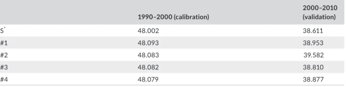
The performance of each candidate solution is reported in Table 3. The CNGA calibration reveals that solution #1 is the best‐performing one. However, the other solutions show comparable performance, with very marginal FSR differences between 0.01 and 0.14. This indicates that each solution works well in specific locations across the study area, which enables us to explore the spatial heterogeneity in the relationship between the LC process and its driving forces. Table 3 also shows that the CNGA slightly outperformed the standard GA. This can be explained by the fact that the CNGA decreases the potential of trapping into a local optimum.
Table 4 lists the Euclidean distance between the vectors of each candidate solution. Table 5 shows the al‐ location mismatches between each solution during the period 1990–2000. Both tables reveal that Solution #1 is remarkably different from Solution #3. According to Table 2, Solution #1 allocates new urban areas far from
TA B L E 3 The fuzziness similarity rate for calibration and validation
1990–2000 (calibration) 2000–2010 (validation) S* 48.002 38.611 #1 48.093 38.953 #2 48.083 39.582 #3 48.082 38.810 #4 48.079 38.877
*Single solution (using the standard GA).
TA B L E 2 Results of optimal parameter weights
α X1 X2 X3 X4 X5 X6 X7 X8 X9 σ S* −5.546 0.964 0.227 −1.562 −1.005 −5.046 −4.174 1.729 2.472 9.809 0.017 #1 −5.734 1.109 0.185 −1.672 −0.949 −5.429 −4.562 1.693 2.572 10.027 0.009 #2 −4.994 0.557 0.079 −1.133 −0.921 −3.975 −3.321 1.696 2.187 9.243 0.023 #3 −5.040 1.467 −0.727 −0.063 −0.989 −3.610 −3.461 0.564 2.182 9.763 0.094 #4 −5.369 0.987 −0.429 −0.894 −0.892 −4.838 −3.838 1.155 1.978 10.117 0.026 STD** 0.343 0.375 0.430 0.669 0.041 0.825 0.556 0.539 0.248 0.393 0.038
existing cities, and near to roads. In contrast, the Solution #3 allocation process is mainly affected by the slope, the distance to major cities, and the number of local urban neighbors. Figure 3 confirms that Solution #3 works better within urban cores, whereas Solution #1 outperforms Solution #3 in rural areas.
In order to find the locations in which each solution outperforms the others, we adopted a moving window approach. The window dimensions were first estimated through an incremental spatial autocorrelation test. This test measures the global Moran’s index at a series of increasing distances, measuring the intensity of clustering and/or dispersion. The higher positive z‐score values when statistically significant, the higher the degree of clus‐ tering for a given distance (Tighe, Fillingim, & Hurley, 2014). Figure 4 depicts the incremental spatial autocor‐ relation peaking at a distance of about 12,000 m. Consequently, we set the dimensions of the moving window to 12,000 × 12,000 m (120 × 120 cell).
Figure 5 shows that Solution #4 is the best solution within dense urban areas (i.e., Liege, Charleroi, and Mons). Solution #3 better suits medium‐sized cities (e.g., Namur), as well as smaller urban nodes. According to Table 5, both solutions are closer to each other than Solutions #1 and #2. The major differences between Solutions #3 and #4 are the magnitude of geophysical factors (i.e., elevation and slope, the effect of highways, and the immediate urban neighbors). The magnitude of elevation and slope in Solution #3 is much stronger than in Solution #4, imply‐ ing that new developments in Solution #3 areas are more affected by the elevation and slope degree. The effect of highways on urban development within Solution #3 areas is marginal compared to Solution #4 areas. Solution #2 best fits development in border areas, especially the border with Flanders (north Belgium) and Brussels regions. Solution #1 is most adapted to rural areas, which are relatively isolated and fragmented. This explains the strong role of distance to various road classes for Solution #1. This is especially the case for the distance to secondary and local roads, as many of these small settlements are only accessible by local roads. Solution #1 also shows a lower neighborhood effect than other solutions according to σ (Equation 1), meaning that these areas are largely affected by discontinuous urban development and landscape fragmentation, while the other three solutions, and especially Solution #3, are oriented toward more aggregated built‐up areas.
TA B L E 4 Euclidean distance between each candidate solution
#1 #2 #3 #4
#1 0 2.360 3.172 1.630
#2 2.360 0 2.083 1.660
#3 3.172 2.083 0 1.817
#4 1.630 1.660 1.817 0
TA B L E 5 Mismatches between the allocations of new urban cells between each candidate solution (% of the
total changed cells during the period 1990–2000, i.e., 17,010 cells in total)
#1 #2 #3 #4
#1 0 1,166 (6.9) 3,110 (18.3) 2,308 (13.6)
#2 1,166 (6.9) 0 3,090 (18.2) 2,359 (13.9)
#3 3,110 (18.3) 3,090 (18.2) 0 1,352 (7.9)
F I G U R E 3 Mismatches between Solutions #1 and #3, and #2 and #3 during the calibration interval 1990–
4 | CONCLUSIONS AND FUTURE WORK
This article has explored the advantage of implementing niching methods that extend the genetic algorithm to identify multiple solutions in LC models. We have implemented the CNGA to calibrate a cellular automata LC model. The CNGA allowed us to distinguish four divergent optimal solutions with comparable performance re‐ sults, evaluated by means of the fuzziness similarity rate.
We believe that this work is important for many reasons. First, finding multiple optima is important to dis‐ cover the relationship between specific subspaces and LC drivers. Our results provide evidence that the effect of each driver changes magnitude in the various subspaces. Second, the existence of competing solutions should be
F I G U R E 4 Incremental spatial autocorrelation
F I G U R E 5 Locations where each solution outperforms others over Wallonia during the calibration interval
considered in future forecasting, as each solution may not be stable over time. The case study shows that Solution #2 performs better than other solutions during the period 2000–2010, while it was Solution #1 that performed best during the period 1990–2000. This opens an avenue toward sensitivity analysis, taking into consideration various solutions for future predictions. Third, the findings are important for policy makers, as they will help eval‐ uate and adopt the location‐based spatial planning strategies for a given region considering several subspaces and their specificities.
Many further research directions are raised by this study. We examined one of the common approaches to searching for several optimal solutions. As mentioned above, many other algorithms can be employed to discover several solutions. Future studies could examine other algorithms to identify their advantages and shortcomings. In this study, we have used a moving window to define several zones and determine which solution works best for each subspace. The z score of the global Moran’s index for incremental distances has been introduced to deter‐ mine the appropriate window dimensions. More research on how to subdivide large areas into smaller geographic zones needs to be conducted in order to finetune the partition of a given space into subspaces where the various solution are most adapted.
ACKNOWLEDGMENTS
The research was funded through the European Regional Development Fund – FEDER (Wal‐e‐Cities Project).
ORCID
Ahmed Mustafa http://orcid.org/0000‐0002‐1592‐6637
Amr Ebaid https://orcid.org/0000‐0002‐2093‐9790
Jacques Teller http://orcid.org/0000‐0003‐2498‐1838
REFERENCES
Achmad, A., Hasyim, S., Dahlan, B., & Aulia, D. N. (2015). Modeling of urban growth in tsunami‐prone city using logistic regression: Analysis of Banda Aceh, Indonesia. Applied Geography, 62, 237–246.
Al‐Ahmadi, K., See, L., Heppenstall, A., & Hogg, J. (2009). Calibration of a fuzzy cellular automata model of urban dynam‐ ics in Saudi Arabia. Ecological Complexity, 6, 80–101.
Ando, S., Sakuma, J., & Kobayashi, S. (2005). Adaptive isolation model using data clustering for multimodal function optimization. In Proceedings of the 7th Annual Conference on Genetic and Evolutionary Computation (pp. 1417–1424). Washington, DC: ACM.
Basse, R. M., Omrani, H., Charif, O., Gerber, P., & Bódis, K. (2014). Land use changes modelling using advanced methods: Cellular automata and artificial neural networks. The spatial and explicit representation of land cover dynamics at the cross‐border region scale. Applied Geography, 53, 160–171.
Belgian Federal Government (2013). Statistics Belgium. Retrieved from https://statbel.fgov.be/fr/statistiques/chiffres/ Chen, C. H., Liu, T. K., & Chou, J. H. (2014). A novel crowding genetic algorithm and its applications to manufacturing
robots. IEEE Transactions on Industrial Informatics, 10(3), 1705–1716.
Clarke, K. C., Hoppen, S., & Gaydos, L. (1997). A self‐modifying cellular automaton model of historical urbanization in the San Francisco Bay area. Environment & Planning B, 24, 247–261.
Črepinšek, M., Liu, S.‐H., & Mernik, M. (2013). Exploration and exploitation in evolutionary algorithms: A survey. ACM
Computing Surveys, 45, 1–35.
Das, S., Maity, S., Qu, B.‐Y., & Suganthan, P. N. (2011). Real‐parameter evolutionary multimodal optimization: A survey of the state‐of‐the‐art. Swarm Evolutionary Computing, 1, 71–88.
De Jong, K. A. (1975). An analysis of the behavior of a class of genetic adaptive systems. Ann Arbor, MI: University of Michigan Press.
Feng, Y., Liu, Y., Tong, X., Liu, M., & Deng, S. (2011). Modeling dynamic urban growth using cellular automata and particle swarm optimization rules. Landscape & Urban Planning, 102, 188–196.
Fisher, P., Comber, A., & Wadsworth, R. (2005). Land use and land cover: Contradiction or complement. In P. Fisher & D. Unwin (Eds.), Re‐presenting GIS (pp. 85–98). Chichester, UK: John Wiley & Sons.
García, A. M., Santé, I., Boullón, M., & Crecente, R. (2013). Calibration of an urban cellular automaton model by using sta‐ tistical techniques and a genetic algorithm: Application to a small urban settlement of NW Spain. International Journal
of Geographical Information Science, 27, 1593–1611.
Goldberg, D. E., & Richardson, J. (1987). Genetic algorithms with sharing for multimodal function optimization. In J. J. Grefenstette (Ed.) Proceedings of the Second International Conference on Genetic Algorithms and Their Application (pp. 41–49). Hillsdale, NJ: Lawrence: Erlbaum Associates Inc.
Hall, M. (2012). A cumulative multi‐niching genetic algorithm for multimodal function optimization. International Journal
of Advanced Research in Artificial Intelligence, 1(9), 6–13.
Holland, J. H. (1975). Adaptation in natural and artificial systems. Cambridge, MA: MIT Press.
Li, J. P., Li, X. D., & Wood, A. (2010). Species based evolutionary algorithms for multimodal optimization: A brief review. In
Proceedings of the IEEE Congress on Evolutionary Computation (pp. 1–8). Barcelona, Spain: IEEE.
Liu, Y., Tang, W., He, J., Liu, Y., Ai, T., & Liu, D. (2015). A land‐use spatial optimization model based on genetic optimization and game theory. Computers, Environment & Urban Systems, 49, 1–14.
Mahfoud, S. W. (1992). Crowding and preselection revisited. In R. Manner & B. Manderick (Eds.), Parallel problem solving
from nature (pp. 27–36). Amsterdam, the Netherlands: Elsevier Science.
Mahfoud, S. W. (1993). Simple analytical models of genetic algorithms for multimodal function optimization. In Proceedings
of the 5th International Conference on Genetic Algorithms (p. 643). San Francisco, CA: Morgan Kaufmann Publishers Inc.
Mahiny, A. S., & Clarke, K. C. (2012). Guiding SLEUTH land‐use/land‐cover change modeling using multicriteria evalua‐ tion: Towards dynamic sustainable land‐use planning. Environment and Planning B, 39, 925–944.
Mengshoel, O. J., & Goldberg, D. E. (2008). The crowding approach to niching in genetic algorithms. Evolutionary
Computing, 16, 315–354.
Mileva, S., Suzana, D., Miloš, K., & Branislav, B. (2015). Modeling urban land use changes using support vector machines.
Transactions in GIS, 20, 718–734.
Miller, B. L., & Shaw, M. J. (1996). Genetic algorithms with dynamic niche sharing for multimodal function optimization. In
Proceedings of IEEE International Conference on Evolutionary Computation (pp. 786–791). Nagoya, Japan: IEEE.
Mustafa, A., Cools, M., Saadi, I., & Teller, J. (2017). Coupling agent‐based, cellular automata and logistic regression into a hybrid urban expansion model (HUEM). Land Use Policy, 69, 529–540.
Mustafa, A., Heppenstall, A., Omrani, H., Saadi, I., Cools, M., & Teller, J. (2018). Modelling built‐up expansion and densifi‐ cation with multinomial logistic regression, cellular automata and genetic algorithm. Computers, Environment & Urban
Systems, 67, 147–156.
Mustafa, A., Rienow, A., Saadi, I., Cools, M., & Teller, J. (2018). Comparing support vector machines with logistic regres‐ sion for calibrating cellular automata land use change models. European Journal of Remote Sensing, 51(1), 391–401. Mustafa, A., Saadi, I., Cools, M., & Teller, J. (2015). Modelling uncertainties in long‐term predictions of urban growth: A
coupled cellular automata and agent‐based approach. In Proceedings of the 14th International Conference on Computers
in Urban Planning and Urban Management. Cambridge, MA.
Petrowski, A. (1996). A clearing procedure as a niching method for genetic algorithms. In Proceedings of the IEEE
International Conference on Evolutionary Computation (pp. 798–803). Nagoya, Japan: IEEE.
Petrowski, A. (1997). An efficient hierarchical clustering technique for speciation. Evry, France: Institute National des Telecommunications.
Pijanowski, B. C., Tayyebi, A., Doucette, J., Pekin, B. K., Braun, D., & Plourde, J. (2014). A big data urban growth simulation at a national scale: Configuring the GIS and neural network based land transformation model to run in a high perfor‐ mance computing (HPC) environment. Environmental Modeling & Software, 51, 250–268.
Sheng, W., Chen, S., Sheng, M., Xiao, G., Mao, J., & Zheng, Y. (2016). Adaptive multi‐subpopulation competition and multi‐ niche crowding‐based memetic algorithm for automatic data clustering. IEEE Transactions on Evolutionary Computing,
20, 838–858.
Singh, G., & Deb, K. (2006). Comparison of multi‐modal optimization algorithms based on evolutionary algorithms. In
Proceedings of the 8th Annual Conference on Genetic and Evolutionary Computation (pp. 1305–1312). Seattle, WA: ACM.
Tighe, P. J., Fillingim, R. B., & Hurley, R. W. (2014). Geospatial analysis of hospital consumer assessment of healthcare providers and systems pain management experience scores in U.S. hospitals. Pain, 155(5), 1016–1026.
Turner, B. L., Lambin, E. F., & Reenberg, A. (2007). The emergence of land change science for global environmental change and sustainability. Proceedings of the National Academy of Sciences of the USA, 104, 20666–20671.
van Vliet, J., Bregt, A. K., Brown, D. G., van Delden, H., Heckbert, S., & Verburg, P. H. (2016). A review of current calibra‐ tion and validation practices in land‐change modeling. Environmental Modeling & Software, 82, 174–182.
Ward, D. P., Murray, A. T., & Phinn, S. R. (2000). A stochastically constrained cellular model of urban growth. Computers,
White, R., & Engelen, G. (2000). High‐resolution integrated modelling of the spatial dynamics of urban and regional sys‐ tems. Computers, Environment & Urban Systems, 24, 383–400.
Wu, F. (2002). Calibration of stochastic cellular automata: The application to rural–urban land conversions. International
Journal of Geographical Information Science, 16, 795–818.
Yang, X., Zheng, X.‐Q., & Chen, R. (2014). A land use change model: Integrating landscape pattern indexes and Markov‐ CA. Ecological Modeling, 283, 1–7.
Yin, X., & Germay, N. (1991). Investigations on solving the load flow problem by genetic algorithms. Electric Power Systems
Research, 22, 151–163.
Yin, X., & Germay, N. (1993). A fast genetic algorithm with sharing scheme using cluster analysis methods in multimodal function optimization. In R. F. Albrecht, C. R. Reeves, & N. C. Steele (Eds.), Artificial neural nets and genetic algorithms (pp. 450–457). Vienna, Austria: Springer.
How to cite this article: Mustafa A, Ebaid A, Teller J. Benefits of a multiple‐solution approach in land