Automatic Cephalometric X-Ray Landmark
Detection Challenge 2014: A tree-based
algorithm
R. Vandaele, R. Maree, S. Jodogne, and P. Geurts
University of Liege, Belgium, [email protected],
Systems and Modelling Unit (GIGA-R & Department of EE and CS), Sart-Tilman, B34
4000 Liege
Abstract. In this paper, we propose a machine learning based algorithm for the Automatic Cephalometric X-Ray Landmark Detection Challenge. We use Extremely Randomized Forests combined with simple pixel-based multiresolution features. Using 10-fold cross validation, detection rate for some landmarks is reaching 96% under 2.5mm. Results show high variability between the different landmarks: some landmarks are detected with high accuracy while some others appears to be more difficult to detect, probably due to the high variability of their appearance in the dataset.
1
Introduction
Cephalometry is a particular process to analyze the human cranium. It consists in detecting landmarks and measuring the distances and distance ratio between these landmarks in order to detect possible problems or plan intervention treat-ments. It is heavily used in the medical community, but the hard task of manually detect these landmarks makes it a very complicated and time consuming task. This why automated and semi automated methods are currently developped.
Numerous studies have been proposed to solve the problem, but the lack of data to make real comparisons between these studies make the choice of a suitable detection algorithm difficult. The goal of this challenge is thus to propose a fair comparison between landmark detection algorithms and propose a gold standard evaluation dataset for further studies.
The problem of landmark localization in X-Rays is a well-known problem in the litterature. A brief review of these methods is presented in [5]. These methods are mostly based on combinations of template matching and priory knowledge informations. Differences comes in the feature extraction methods: edge dete-cion, Zernike moments,... From the litterature, machine learning tree-based ap-proaches were never used for landmark detection on X-Rays. Machine learning tree-based techniques, and especially Random Forests [2] and Extremely Ran-domized Forests [4] becomes more and more used in the imaging litterature for
II
their ability to correctly handle a large number of features, making possible the use of simple features to recognize complex structures and objects in images. For example, it was used in [6] for cells classification, or in [1] for hand-digit recogniton.
On closest topics, (extremely) randomized forests for classification or regres-sion were recently applied to similar problems: in [8], Stern used Extremely Randomized Forests to detect landmarks on zebrafish. In [3], Criminisi used Random Forests to predict the organ location in three dimensional CTs.
2
Our approach
Our approach follows a supervised classification approach. No matter the algo-rithm used, the goal of supervised classification is to predict the class of a new observation given a dataset of previously classified observations. In this context, we first need to define what is an observation, and which are the classes used in our modelization.
As it is done in [8], one observation corresponds to one pixel on a cephalo-metric X-Ray image. If the position of the landmark on image i is (xi, yi), then
the class of the pixel located at position (x, y) is:
– 1 if distance((x, y), (xi, yi)) ≤ R
– 0 otherwise
One pixel can either be an interest point if it is located at a distance ≤ R to the translated position of the interest point on the image, or not an interest point otherwise. As we have 19 landmarks to detect, it means that we will have to build 19 different models.
One observation corresponds to one pixel located at position (x, y). It is defined by a window of pixel values centered in (x + tx, y + ty) in a radius W , at
6 different resolutions. For our images of size 2400×1935 pixels, these resolutions will be:
2400 2i ×
1935
2i ∀i ∈ [0, 5]
It allows to capture the context of the interest point at different levels. We will thus have a feature vector of size 6 × ((2W + 1)2).
In recapitulation, this approach generates 4 particular parameters:
– W , the size of the windows
– R, the distance to the interest point
– txand ty, the translation. These parameters could allow us to detect
struc-tures near the landmark that are more stable to detect for our algorithm. Its interest is showed in the results section.
III
2.1 Training
One particular problem for training is the size of the dataset: one single image has 2400×1935 pixels, which means 2400×1935 potential observations per image with our modelization. Using complete randomization for data selection led to a completely unbalanced learning problem: compared to the size of the whole image, only a very small part of the image belongs to a landmark class: for a radius R of 2mm, there are 1256 observations that belongs to the landmark class, which means 0.027% of the image. We solved this problem using two approaches:
1. In order to build a model for a specific landmark, we randomly select N points on each image of the training set, where P % of the data will be from the landmark class, and thus (100 − P )% not from the landmark class. The problem is then to be able to have a correct modelization of the rest of the image.
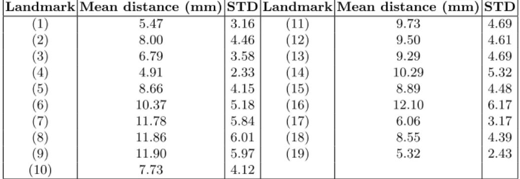
2. Figure 2.1 shows the mean distance of the landmarks to their mean position (obtained by taking the means of every landmark of the training set). From this analysis it is clear that the landmarks are not moving accross the whole image, but on smmaler areas of radius of size 5 − 15mm. This is why, instead of trying to learn the whole image, we chose to only learn observations on a surrounding of 40mm around each landmark. Of course, a similar approach will have to be used for prediction.
Landmark Mean distance (mm) STD Landmark Mean distance (mm) STD (1) 5.47 3.16 (11) 9.73 4.69 (2) 8.00 4.46 (12) 9.50 4.61 (3) 6.79 3.58 (13) 9.29 4.69 (4) 4.91 2.33 (14) 10.29 5.32 (5) 8.66 4.15 (15) 8.89 4.48 (6) 10.37 5.18 (16) 12.10 6.17 (7) 11.78 5.84 (17) 6.06 3.17 (8) 11.86 6.01 (18) 8.55 4.39 (9) 11.90 5.97 (19) 5.32 2.43 (10) 7.73 4.12
Table 1. Mean distance of the landmarks to the mean of their landmark position on the training set
2.2 Model building
Given a learning dataset of dimension m × n, (m observations of n features) classified into two classes, the Extremely Randomized Forests algorithm will build a forest of T decision trees.
IV
Each tree is built using the whole dataset of observations. The goal of the extremely randomized tree algorithm is to create a tree progressively creat-ing hyper-rectangular partitions of the dataset separatcreat-ing the two classes. The important point about (extremely) randomized forests is that one tree is not searching for the best possible partitioning. It was shown in [2] and [4] that using randomness and ensemble methods instead of trying to find the optimal partitioning of the training data leads to better accuracy and fewer overfitting problems during the prediction phase.
For the top node, K features are randomly chosen among the n features available. In the Extra-Trees algorithm, with each feature comes a split chosen randomly within the range of variation of this feature. The pair (feature,split) giving the best partitioning is then chosen to create the new two partitions. As long as there is at least 2 observations in the dataset, and the maximal depth D is not reached, the children nodes will use the same paritioning algorithm with the dataset inside their corresponding partition.
2.3 Landmark Detection
Given PT, the set of positions of the landmark in the training data, XT the
position of the landmarks on the X axis (first column of PT) and YT the positions
of the landmark on the Y axis (second column of PT), we generate 16σ(X)σ(Y )
observations on random positions generated by the multivariate normal law:
N ( ¯PT, Cov(PT))
Statistically speaking, this will allow us to get an interesting landmark / non-landmark ratio, because it reduces the probability of generating non-non-landmark positions. Moreover, it allowed to considerably speedup the algorithm, because of the fact that we do not predict each pixel of the image. For obvious compu-tational reasons, this way of data selection was not integrated to training: this would have mean that data had to be reselected for each step of the 10-CV.
The predicted landmark position is the median position of the observations detected as landmark with the highest probability (the observations detected as landmarks by the biggest number of trees).
3
Results
Because of the numerous parameters we had to explore for each landmark, a complete analysis of all of these parameters would be too long for this paper: for each landmark, different optimums were obtained for the different performance criterions used. This is especially true for the parameters R, txand ty, where the
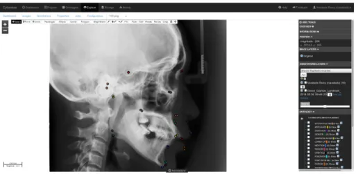
optimal parameters are different according to the optimization criterion used. Visual interpretation of the results was done using Cytomine [7], a web-service allowing easier analysis of landmarks-annotated images. An example of its interface is shown in Figure 3. With this interface, it was easy to interpret
V
Fig. 1. Cytomine framework
the results and compare them to the ground truth data: the problematic areas and landmarks, the variation of the position of a landmark accross the images,... For the tree parameters, best results were obtained when the depth was not bound, and when the number of tested features was the square root of the total number of features. We thus use 500 trees without depth limitation, and K = 44. tx, ty were jointly tested for values of 0.8, 1.6, 3.2, 6.4, 12.8 and 25.6mm, for positive and negative translations. They were the first tested using R = 1mm and P = 33%. Then R was tested for distances of 0.2, 0.5, 0.7, 1, 1.2, 1.5, 1.7, 2, 2.5 and 3mm for each image (P fixed to 33% and tx, ty fixed to the previously obtained value. Finally, P was tested for proportions of 10, 20, 30, 33.33, 40, 50, 60, 70, 80 and 90%. This final version of our algorithm roughly represents 2000 cross-validation jobs for this paremeter selection.
In this section, we want to show the influence of our translation parameters. Table 2 shows optimized results without considering any translation, while table 3 shows the best results using translations. For table 3, we showed the best translations obtained for the 2.5mm criterion to give an idea of their positions. There is a clear improvement for some landmmark by using translations. The sella point for example, is more correctly detected. We notice however that two particular points are not correctly detected, even at higher acceptance criterion: the supramentale and the gonion. Given the good results obtained on other landmarks and other inconclusive tests we have made on these two points, our conclusion is that either the dataset is not able to capture the high variability of the surrounding of these landmarks or there was some errors during the manual annotation process.
VI
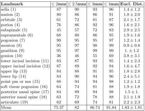
Landmark ≤ 2mm ≤ 2.5mm ≤ 3mm ≤ 4mm Eucl. Dist. sella (1) 87 90 93 96 1.4 ± 1.2 nasion (2) 80 86 86 91 1.8 ± 2.0 orbitale (3) 61 72 81 87 2.1 ± 1.7 porion (4) 76 86 92 96 1.6 ± 2.1 subspinale (5) 45 57 72 83 2.9 ± 2.5 supramentale (6) 68 80 86 95 1.9 ± 1.6 pogonion (7) 90 95 95 97 1.2 ± 1.4 menton (8) 95 97 98 99 0.9 ± 0.8 gnathion (9) 95 97 99 99 1. ± 1.2 gonion (10) 36 46 55 69 3.8 ± 3.1 lower incisal incision (11) 83 87 93 95 1.4 ± 2.3 upper incisal incision (12) 87 89 92 94 1.6 ± 4.7 upper lip (13) 84 88 91 95 1.8 ± 2.8 lower lip (14) 84 90 94 96 2.4 ± 5.1 point pm or mn (15) 88 94 94 98 1.2 ± 1.2 soft tissue pogonion (16) 64 74 81 88 1.9 ± 1.8 posterior nasal spine (17) 84 89 94 98 1.5 ± 1. anterior nasal spine (18) 63 72 78 88 2.1 ± 1.9 articulate (19) 62 69 74 81 2.2 ± 2.3 Mean 75.37 82 86.74 91.84 1.83 ± 1.81
Table 2. Results with no translations
Landmark ≤ 2mm ≤ 2.5mm ≤ 3mm ≤ 4mm Eucl. Dist. tx (mm) ty (mm) sella (1) 95 96 96 97 1.21 ± 1.92 3.2 1.6 nasion (2) 78 83 86 90 1.86 ± 2.06 0 0 orbitale (3) 63 75 83 92 2.06 ± 1.50 0.8 −6.4 porion (4) 77 86 92 97 1.53 ± 1.22 0 0 subspinale (5) 54 63 71 83 2.78 ± 2.20 0 1.6 supramentale (6) 71 78 86 95 1.84 ± 1.56 −1.6 −0.8 pogonion (7) 89 94 97 99 1.21 ± 1.30 0 0 menton (8) 94 97 98 100 0.94 ± 0.80 0.8 −0.8 gnathion (9) 97 99 99 100 0.91 ± 0.69 −3.2 −0.8 gonion (10) 38 48 56 66 3.76 ± 2.85 1.6 1.6 lower incisal incision (11) 89 92 95 97 1.44 ± 2.35 −1.6 1.6 upper incisal incision (12) 88 92 95 97 1.29 ± 3.27 3.2 −6.4 upper lip (13) 84 89 93 95 1.56 ± 2.08 0 −0.8 lower lip (14) 87 93 96 99 1.45 ± 2.36 −0.8 −0.8 point pm or mn (15) 88 92 95 98 1.19 ± 1.07 1.6 1.6 soft tissue pogonion (16) 67 75 83 91 1.94 ± 1.80 −0.8 −1.6 posterior nasal spine (17) 83 90 95 98 1.38 ± 1.06 0.8 0.8 anterior nasal spine (18) 67 78 84 91 2.01 ± 1.56 −3.2 0 articulate (19) 65 74 79 86 2.28 ± 2.06 1.6 3.2 Mean 77.58 83.89 88.37 93.21 1.72 ± 1.77
VII
Figure 3 shows the position of the gonion on different images. It seems that the local position of the landmark does not fit the same structure on each of the images.
Fig. 2. Gonion surroundings for training set images 10,20,30 and 40. In red, the position of the gonion landmark
4
Conclusion
We showed that it was possible to accurately detect some of the landmarks using a combination of Extremely Randomized Forests and simple features. We think that given the small dataset and the variance of the landmarks between the images, these results are promising in comparison to existing algorithms. High level features such as Zernike moments can accurately describe an image or a window, but are slow to compute, and this can become very painful in an application such as landmark detection, where numerous positions will typically have to be tested (or more precisely, the more will be tested, the more accurate will be the algorithm).
We think that the main problem for our approach is the lack of data: for some landmarks, 100 images does not grasp the variability of the possible landmark structures. Moreover, it seems that some landmarks do not especially correspond to specific shapes or structures, but more to positions or interestections.
For our algorithm, further improvement could likely be brought by consider-ing the whole structure made by the 19 landmarks. Further improvement could
VIII
also be brought by considering different values of W at each of the different resolutions.
References
1. Simon Bernard, S´ebastien Adam, and Laurent Heutte. Using random forests for handwritten digit recognition. In Document Analysis and Recognition, 2007. ICDAR 2007. Ninth International Conference on, volume 2, pages 1043–1047. IEEE, 2007. 2. Leo Breiman. Random forests. Machine learning, 45(1):5–32, 2001.
3. Antonio Criminisi, Jamie Shotton, Duncan Robertson, and Ender Konukoglu. Re-gression forests for efficient anatomy detection and localization in ct studies. In Med-ical Computer Vision. Recognition Techniques and Applications in MedMed-ical Imaging, pages 106–117. Springer, 2011.
4. Pierre Geurts, Damien Ernst, and Louis Wehenkel. Extremely randomized trees. Machine learning, 63(1):3–42, 2006.
5. Amandeep Kaur and Chandan Singh. Automatic cephalometric landmark detection using zernike moments and template matching. Signal, Image and Video Processing, pages 1–16, 2013.
6. Rapha¨el Mar´ee, Pierre Geurts, and Louis Wehenkel. Random subwindows and ex-tremely randomized trees for image classification in cell biology. BMC Cell Biology, 8(Suppl 1):S2, 2007.
7. Rapha¨el Mar´ee, Loic Rollus, Gilles Louppe, Olivier Caubo, Natacha Rocks, Sandrine Bekaert, Didier Cataldo, and Louis Wehenkel. A hybrid human-computer approach for large-scale image-based measurements using web services and machine learning. In Proceedings IEEE International Symposium on Biomedical Imaging. IEEE, 2014. 8. Olivier Stern, Rapha¨el Mar´ee, Jessica Aceto, Nathalie Jeanray, Marc Muller, Louis Wehenkel, and Pierre Geurts. Automatic localization of interest points in zebrafish images with tree-based methods. In Pattern Recognition in Bioinformatics, pages 179–190. Springer, 2011.