HAL Id: dumas-01101356
https://dumas.ccsd.cnrs.fr/dumas-01101356
Submitted on 8 Jan 2015HAL is a multi-disciplinary open access
archive for the deposit and dissemination of sci-entific research documents, whether they are pub-lished or not. The documents may come from teaching and research institutions in France or abroad, or from public or private research centers.
L’archive ouverte pluridisciplinaire HAL, est destinée au dépôt et à la diffusion de documents scientifiques de niveau recherche, publiés ou non, émanant des établissements d’enseignement et de recherche français ou étrangers, des laboratoires publics ou privés.
assess marine protected areas
Auriane Virgili
To cite this version:
Auriane Virgili. Predicting variations in coastal seabird habitats to assess marine protected areas. Agricultural sciences. 2014. �dumas-01101356�
Université de La Rochelle 23, avenue Albert Einstein BP 33060 - 17031 La Rochelle -
05 46 45 91 14 05 46 44 93 76 AGROCAMPUS OUEST
Centre de Rennes 65 rue de Saint Brieuc
35042 Rennes Cedex 02 23 48 50 00
02 23 48 55 10
Observatoire PELAGIS Pôle analytique, 5 allées de l’Océan,
17000 La Rochelle 05 46 44 99 10 05 46 44 99 45
Mémoire de Fin d'Etudes
Diplôme d’Ingénieur de l’Institut Supérieur des Sciences Agronomiques,
Agroalimentaires, Horticoles et du Paysage
Année universitaire 2013 – 2014
Spécialisation Halieutique – Option Ressources et Écosystèmes Aquatiques
Predicting variations in coastal seabird habitats to assess
marine protected areas
Auriane VIRGILI
Volet à renseigner par l’enseignant responsable de l’option/spécialisation Bon pour dépôt (version définitive)
Date : …./…/… Signature : Autorisation de diffusion : Oui Non
Devant le jury : Soutenu à Rennes le : 10/09/2014
Sous la présidence de : Olivier LE PAPE
Maître de stage : Vincent RIDOUX (Professeur et Directeur de l’UMS PELAGIS)
Enseignants référents : Didier GASCUEL et Olivier LE PAPE (AGROCAMPUS OUEST) Autre membre du jury : Pierre PETIGAS (IFREMER Nantes)
CNRS - Centre national de la recherche scientifique
3, rue Michel-Ange 75794 Paris cedex 16 - France
01 44 96 40 00 01 44 96 53 90
"Les analyses et les conclusions de ce travail d'étudiant n'engagent que la responsabilité de son auteur et non celle d’AGROCAMPUS OUEST". CEBC – CNRS
Villiers en Bois BP 14 79360 Beauvoir/Niort 05 49 09 61 11
Fiche de diffusion du mémoire
A remplir par l’auteur(1) avec le maître de stage.Aucune confidentialité ne sera prise en compte si la durée n’en est pas précisée.
Préciser les limites de la confidentialité (2) :
Confidentialité absolue : oui non
(ni consultation, ni prêt)
Si oui 1 an 5 ans 10 ans
A l’issue de la période de confidentialité ou si le mémoire n’est pas confidentiel, merci de renseigner les éléments suivants :
Référence bibliographique diffusable(3) : oui non
Résumé diffusable : oui non
Mémoire consultable sur place : oui non
Reproduction autorisée du mémoire : oui non
Prêt autorisé du mémoire : oui non
……….
Diffusion de la version numérique : oui non
Si oui, l’auteur(1) complète l’autorisation suivante :
Je soussignée Auriane VIRGILI, propriétaire des droits de reproduction dudit résumé, autorise toutes les sources bibliographiques à le signaler et le publier.
Date : Signature :
Rennes,
Le maître de stage(4), L’auteur(1),
L’enseignant référent,
(1) auteur = étudiant qui réalise son mémoire de fin d’études
(2) L’administration, les enseignants et les différents services de documentation d’AGROCAMPUS OUEST s’engagent à respecter cette confidentialité.
(3) La référence bibliographique (= Nom de l’auteur, titre du mémoire, année de soutenance, diplôme, spécialité et spécialisation/Option)) sera signalée dans les bases de données documentaires sans le résumé.
Remerciements
Je tiens avant tout d’abord à remercier mon maître stage, Vincent Ridoux, pour m’avoir offert la possibilité de travailler avec lui sur un sujet qui me tenait à cœur mais aussi d’avoir été présent tout au long de mon stage et de me permettre de poursuivre mon projet professionnel grâce à une thèse.
Je remercie également Charlotte, Emeline, Sophie et Amandine avec qui se fut un réel plaisir de travailler durant ces 6 mois de stage. Elles m’ont soutenue et apporté leur aide tout au long du stage et pour cela je les en remercie.
Merci à toute l’équipe de l’Observatoire PELAGIS pour m’avoir accueillie aussi chaleureusement et aidée en cas de besoin.
Merci également à tous les observateurs des campagnes SAMM sans qui ce travaille n’aurait pas pu être réalisé.
Merci à Previmer qui nous a fourni les données environnementales essentielles à la modélisation d’habitats.
Je remercie également AGROCAMPUS OUEST et les professeurs du pôle halieutique, ainsi que mes tuteurs de stage Olivier Le Pape et Didier Gascuel pour m’avoir permis de réaliser un tel stage et surtout de m’avoir permis d’acquérir les compétences nécessaires à sa réalisation.
Enfin, je remercie Mathilde, Charlotte, Anne et Marie, les doctorantes du bâtiment ILE, pour leur accueil et leur soutien et je leur dis à très bientôt !
Synthèse étendue
Contexte
Les oiseaux marins sont souvent considérés comme des indicateurs de la composition et de la productivité d’un écosystème (Zacharias and Roff, 2001) car ce sont des prédateurs de hauts niveaux trophiques très sensibles aux conditions environnementales (Piatt et al., 2007). En effet, un manque de nourriture, une pollution ou un disfonctionnement quelconque de l’écosystème se traduit généralement par une diminution de l’abondance des oiseaux et de leur progéniture (Furness and Camphuysen, 1997) par réduction de leur survie ou modification de leur distribution. En outre, leur étude dans leur milieu naturel est relativement aisée car ils sont facilement observables (de visu ou par télémétrie) et s’agrègent naturellement dans les zones de fortes productions marines (Piatt et al., 2007).
Pour se nourrir, les oiseaux de mer sont soumis à de fortes pressions de sélection et doivent donc adapter leurs stratégies d’utilisation de la ressource et des habitats pour maximiser leurs apports nutritionnels et minimiser leurs coûts énergétiques durant leurs périodes d’alimentation (Chaurand and Weimerskirch, 1994). Afin de comprendre comment les oiseaux utilisent leurs habitats, les modèles sont couramment utilisés car ils permettent de corréler la distribution spatiale des oiseaux et les variables environnementales (Vilchis et
al., 2006 ; Mannocci, et al., 2014). En outre, ces modèles sont de plus en plus utilisés pour établir des plans de conservation et de gestion des espèces et des écosystèmes car ils permettent de prédire la distribution des espèces et leurs réponses face aux changements environnementaux, qu’ils soient climatiques ou anthropiques (Bailey and Thompson, 2009; Cheung et al., 2009).
La conservation des espèces et le maintien de la diversité biologique est un enjeu majeur pour les états membres de l’Union Européenne. C’est pour cette raison que, dès 1992, le réseau de sites Natura 2000 (N2000), basé sur les directives Oiseaux (Parlement Européen, 2009) et Habitats Faune et Flore (Parlement européen, 1992), a été mis en place. Pour répondre aux exigences de ce réseau, la France, à travers l’Agence des Aires Marines Protégées, à mis en place un programme d’acquisition de données sur la mégafaune marine afin de faire un inventaire de la faune présente ainsi qu’une évaluation des sites N2000 et autres sites de conservation établis ou prévus sur les côtes françaises métropolitaines.
Objectifs
Dans cette étude, nous nous sommes concentrés sur certaines espèces emblématiques de côtes françaises telles que les sternes (essentiellement sterne pierregarin Sterna hirundo, sterne naine Sterna albifrons et sterne caugek Sterna sandvicensis), goélands (essentiellement, goéland argenté Larus argentatus, goéland leucophée L. michahellis, goéland brun L. fuscus et goéland marin L. marinus), cormorans (grand cormoran
Phalacrocorax carbo et cormoran huppé P. aristotelis). Ces espèces sont qualifiées de
côtières car elles ont un lien biologique et physique à la côte qui les oblige à retourner quotidiennement sur la terre ferme, que se soit pour incuber leurs œufs, nourrir leur progéniture ou bien se reposer. Nous ajoutons à cette première série d’espèces les plongeons (plongeons arctique, catmarin et imbrin Gavia arctica, G. stellata, G. immer) et les macreuses (macreuse brune Melanitta fusca et macreuse noire M. nigra). Dans les deux cas, il s’agit d’espèces principalement hivernantes sur les côtes françaises dont l’habitat est littoral sans pour autant que ces oiseaux reviennent périodiquement à terre. L’étude ne porte pas sur les nombreuses autres espèces encore plus littorales qui utilisent principalement l’estran.
Le but de l’étude était de déterminer, à partir de données d’observation d’oiseaux, les mécanismes qui influencent le plus la distribution des oiseaux marins le long des côtes ouest et nord de la France. En outre, nous avons cherché à déterminer les effets des variations, notamment saisonnières, de ces mécanismes dans le but de proposer une première
évaluation des sites de protection établis ou prévus le long des côtes françaises. Cette évaluation repose sur le critère de la Directive Oiseaux indiquant qu’un site hébergeant au moins 1% de la population ‘nationale’1 d’une espèce devrait être désigné comme Zone de
Protection Spéciale (ZPS).
Méthode
Les données que nous avons utilisées pour la modélisation sont issues de deux campagnes d’observation aérienne, dénommées SAMM (Suivi Aérien de la Mégafaune Marine), réalisées durant l’hiver 2011/2012 et l’été 2012 en Manche et dans le Golfe de Gascogne. A partir de ces données, nous avons créé des groupes d’espèces pour faciliter les analyses et pour palier la difficulté d’identification de certaines espèces proches lors des survols.
Pour modéliser les habitats, nous avons utilisé des Modèles Additifs Généralisés (GAMs). Deux types de variables ont été sélectionnées pour les modèles, des variables physiographiques statiques qui reflètent la bathymétrie et la nature du substrat (pente, profondeur, distance à la côte sableuse ou rocheuse et distance à la colonie) et des variables océanographiques dynamiques qui décrivent les masses d’eau (température de surface, anomalie de hauteur d’eau et courants). Pour les variables océanographiques, nous avons utilisé deux résolutions temporelles à 7 jours et 28 jours (moyennées respectivement sur les 6 et 27 jours précédant le jour échantillonné durant la campagne) pour tenir compte de possibles décalages entre une condition océanographique donnée et son effet sur les niveaux trophiques intermédiaires. A partir de ces variables, une fois les valeurs extrêmes et les observations correspondant à de mauvaises conditions d’observation enlevées, nous avons sélectionné le modèle qui expliquait le mieux la distribution des oiseaux [meilleure déviance et plus faible indice de validation croisée généralisée (GCV)].
Par la suite, ce modèle nous a permis de prédire la distribution de chacun des groupes d’espèces étudiés sur une zone plus étendue que notre zone d’étude. Les prédictions ont été faites sur les deux périodes de campagne (hiver 2011/2012 et été 2012) afin de comparer nos sorties de modèles aux observations faites pendant les campagnes.
Pour finir, nous nous sommes servis des prédictions pour fournir, pour chaque aire marine protégée, site du réseau Natura 2000 ou non, une mesure de son importance pour la protection de chacune des espèces d'oiseaux de mer côtiers (% de l’abondance prédite dans les limites de l’AMP par rapport à l’abondance prédite dans la superficie totale de la zone d’étude ; Fig.i).
Résultats et discussion
Grâce aux survols aériens, sans prendre en compte les transects parcourus dans de mauvaises conditions de vol, 28 068 km ont été échantillonnés en hiver et 31 427 km en été ce qui représentait un total de 2 459 observations d’oiseaux côtiers en hiver et 3 318 en été, utilisées pour les analyses de ce travail.
Les espèces étudiées ont été rencontrées majoritairement dans les strates côtière et néritique de Manche et d’Atlantique durant les deux saisons mais les macreuses et plongeons étaient presque uniquement présents en hiver, et sur les côtes de la Manche pour ces derniers.
1 Il s’agit ici de l’ensemble des individus d’une même espèce présents dans les eaux sous juridiction française. Cette définition
Fig. i. – Schéma explicatif de la démarche expérimentale (exemple du groupe goélands argenté/ leucophée en hiver).
Nos modèles d’habitats présentaient une déviance comprise entre 24,5 et 62,2%, ce qui indique la relative robustesse de nos modèles. A l’exception des plongeons, pour lesquels la profondeur représentait le paramètre déterminant le plus leur distribution (à 38,9%), toutes les autres espèces étaient majoritairement influencées par la distance à la côte la plus proche, souvent avec une inversion entre la côte sableuse et la côte rocheuse selon la saison. Par exemple, les densités de sternes étaient négativement corrélées à la côte rocheuse en hiver et à la côte sableuse en été. Cette inversion s’explique majoritairement par la localisation des colonies en été qui, selon les espèces, sont établies soit les sur les côtes sableuses (cas des sternes), soit sur les côtes rocheuses (cas des goélands). En plus de la distance à la côte, nous avons déterminé les covariables physiographiques et océanographiques qui influencent dans une moindre part la distribution saisonnière de chaque groupe d’espèce. En hiver par exemple, la distribution des goélands gris (goélands argenté et leucophée) était nettement influencée par la distance à la côte sableuse (à 62,5%), aux courants (à 18,4%), à la température moyenne de surface (à 10,8%) et aux variations de cette température (à 8,4%).
Données d’observation
Données d’observation faites à partir de survols aériens
Construction du modèle
GAM g(μ) = α + Σ fi(Xi)
Selection du modèle Comparaison des modèles contenant toutes les combinaisons possibles de 4 variables environnementales non colinéaires sur la base
des GCV minimum
Prédictions
Les prédictions dans la gamme des conditions environnementales
Estimation de l’incertitude
Carte d’incertitude associée à la prédiction basée le coefficient de variation
Evaluation des AMPs
Carte d’évaluation des AMP (seuil de 1%) Variable réponse μ : moyenne de la variable réponseY (nombre d’individus) Variables explicatives fi(Xi) : fonctions non paramétriques des covariables g() : fonction de lien
En ce qui concerne les prédictions, les plus fortes densités des espèces étudiées étaient majoritairement concentrées près des côtes notamment autour des iles, dans les estuaires, les baies ou près des colonies. Pour les goélands et les sternes, qui peuvent être observées plus au large, des patrons de distribution étaient observés avec une absence notable des goélands au large des côtes landaises en été et une quasi absence des sternes le long des côtes du Golfe de Gascogne en hiver.
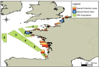
Après évaluation des sites protégés que sont les parcs naturels marins (PNM), les zones de protection spéciales (ZPS) et les propositions de grandes zones pour l’établissement de des futurs sites Natura 2000 au large, il s’est avéré que ces dernières propositions au large ne concernent pas les espèces côtières. Inversement, il apparaitrait que les PNMs de l’Iroise et des Estuaires Picards et Mer d’Opale soient essentiels à la conservation des espèces côtières, notamment pour les plongeons qui séjournent pour en grands nombres sur les côtes picardes ; ce n’est pas le cas pour le PNM du Bassin d’Arcachon. Concernant les ZPS établies, en considérant toutes les espèces étudiées, il apparaitrait que seules 14 ZPS sur 66 soient pertinentes pour la conservation en mer des oiseaux marins côtiers. Ces ZPS sont : “Pertuis Charentais-Rochebonne”, “l’Ile d’Yeu”, “Littoral seino-marin”, “Chausey”, “Estuaire de la Loire – Baie de Bourgneuf”, “Trégor Goëlo”, “Estuaires Picards”, “Cap Gris-Nez”, “Ouessant Molène”, “Panache de la Gironde”, “Banc des Flandres”, “Baie du Mont Saint-Michel”, “Mor Braz” et les “Iles d’Houat et d’Hoëdic”. Ce constat plaide pour l’établissement de plus grands sites protégés que ceux désignés jusqu’à présents ou de la gestion étroitement coordonnée des sites existants formant alors un réseau.
Conclusion
Dans cette étude, nous avons utilisé des variables physiographiques et océanographiques pour modéliser les habitats d'oiseaux de mer côtiers à partir de données d’observation récoltées durant deux campagnes aériennes réalisées pour la première fois sur les côtes françaises métropolitaines au cours de deux saisons, hiver et été. Nous avons particulièrement mis l'accent sur les oiseaux marins côtiers que nous avons définis comme des espèces qui ont un lien biologique ou écologique quotidien avec la côte afin d'accomplir certaines fonctions biologiques essentielles comme la nidification, l'élevage des jeunes ou tout simplement pour se reposer. Les résultats des modèles montrent clairement ce lien avec la côte au travers des patrons de distribution, mais ne reflètent pas les emplacements particuliers des colonies. Nous avons également été en mesure de prédire si les oiseaux étaient plutôt à la recherche de structures océanographiques stables ou prévisibles dans le temps ou s’ils étaient capables d’ajuster leurs stratégies d’utilisation du milieu aux variations environnementales à court terme.
Grâce à l’étendue spatiale des campagnes d’observation et des données environnementales, ce travail nous a permis de fournir une première évaluation des aires marines protégées établies au sein du réseau Natura 2000 le long de la Manche et de l'Atlantique Nord-Est. Il s’est avéré que certaines AMPs ne seraient pas pertinentes pour les espèces étudiées, ce qui n’exclut pas qu’elles le soient pour d’autres espèces ou pour ces mêmes espèces dans la partie terrestre de leur budget d’activités. En outre, ce travail devrait être complété par des prévisions à long terme qui pourraient mettre l'accent sur les réponses des oiseaux de mer aux caractéristiques océanographiques variables. Ce travail devrait constituer une base pour aider les gestionnaires à gérer et surveiller les AMP côtières.
Préambule
Cette étude sur les variations saisonnières des habitats d’oiseaux marins côtiers s’inscrit dans un travail d’équipe réalisé au sein de l’observatoire PELAGIS, à la demande de l’Agence des Aires Marines Protégées dans le cadre du projet SAMM (Suivi Aérien de la Mégafaune Marine) du programme PACOMM (Programme d'Acquisition de Connaissances sur les Oiseaux et les Mammifères Marins). Ce programme vise à recueillir des nouvelles données et compléter les données existantes pour évaluer les sites Natura 2000 en mer actuels et informer les gestionnaires sur des zones d’intérêt biologique susceptibles de justifier la désignation de nouveaux sites dans la Zone Economique Exclusive (ZEE) française. Par ailleurs, le programme PACOMM permettra, dans le cadre de la DCSMM (Directive Cadre Stratégie pour le Milieu Marin), d’établir une situation de référence sur les distributions et abondance de la mégafaune marine dans les eaux sous juridiction française ainsi de proposer des dispositifs de suivis efficaces de la mégafaune marine à partir de campagnes aériennes, de campagnes d’observations depuis des bateaux et de suivis télémétriques et acoustiques.
L’ensemble de ce travail, réalisé en collaboration avec Léa David (chef de mission), Ghislain Dorémus (formation des observateurs, observateur), Hélène Falchetto (gestion de bases de données), Charlotte Lambert (modélisation d’habitats), Sophie Laran (estimations d’abondance), Emeline Pettex (organisation opérationnelle du projet, estimations d’abondance et analyse des distributions), Amandine Ricart (analyse double-plateforme), Vincent Ridoux (direction scientifique), Eric Stephan (chef de mission) et Olivier Van Canneyt (aide à la conception du projet, formation des observateurs, observateur), donnera lieu à la rédaction d’un rapport d’évaluation de cette mégafaune marine le long des côtes françaises métropolitaines qui sera fourni à l’Agence des Aires Marines Protégées, dont un des chapitres sera consacré aux habitats des oiseaux marins côtiers.
Le rapport de stage présenté ici préfigure le chapitre qui sera consacré aux habitats des oiseaux marins côtiers et l’article à soumettre ultérieurement dans une revue scientifique internationale.
List of abbreviations
7d / 28d – 7 days / 28 daysA – Average
Dcolony – Distance to the nearest colony Dcoast – Distance to the nearest coast DSC – Distance to the nearest sandy coast DRC – Distance to the nearest rocky coast CV – Coefficient of variation
EEZ – Exclusive Economic Zone EU – European Union
GAM – Generalized Additive Model GLM – Generalized Linear Model Grad – Gradient
SPA – Special Protected Areas MS – Member States
MPA – Marine Protected Area MNP – Marine Nature Parks N2000 – Natura 2000
NAO – North Atlantic Oscillation
SAMM – Suivi Aérien de la Mégafaune Marine / Aerial Census of Marine Megafauna SD – Standard Error
SPA – Special Protected Area SST – Sea Surface Temperature SSH – Sea Surface Height V – Variance
List of Figures
Fig. 1. – Percentage of Pacific sardine in commercial landings and in the diet of seabirds, 1983-92.
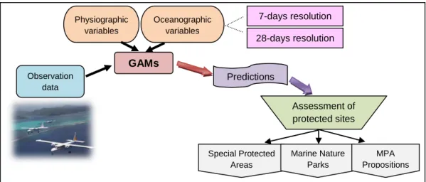
Fig 2. – Experimental approach of the project
Fig. 3. – The study area covers the entire EEZ of mainland France extended to adjacent areas. Fig. 4. – Circulation and currents in the Bay of Biscay and English Channel.
Fig. 5. – Comparison between strip transect and line transect methodologies.
Fig. 6. – Gears used during surveys (Britten Norman 2 aircraft and bubble windows). Fig. 7. – Sampling design: transects planned in coastal, neritic, slope and oceanic strata. Fig. 8. – Distribution map of all seabird sightings throughout the study area.
Fig. 9. – Calculation of SST gradients. Fig. 10. – Stages of habitat modelling.
Fig. 11. – Marine Protected Areas used for the assessment.
Fig. 12. – Forms of smooth functions for the selected covariates for each group of species. Fig. 13. – Predicted relative density for each group of seabirds.
Fig. 14. – Assessment of Special Protected Areas, Marine Nature Parks and Marine Protected areas (MPA) propositions on the French coasts.
List of Tables
Table 1. – Composition of seabird groups.
Table 2. – Environmental covariates used to model seabird habitats. Table 3. – Effort by strata realised during the two surveys.
Table 4. – Number of sightings and individuals in each group by sector and season.
List of Appendices
Appendix A: Presence on the French coasts and breeding periods of each studied species. Appendix B: Monthly effort realised during the two aerial surveys SAMM.
Appendix C: Colonies listed along the French coasts. Appendix D: Maps of average covariate contributions.
Appendix E: Seabird species, number of sightings and number of individuals observed during the two campaigns.
Appendix F: Distribution maps of seabird sightings for each group.
Appendix G: Predicted relative density (number of individuals per km2) for each group of seabirds on the global prediction area.
Appendix H: Uncertainty maps associated to predictive relative density of each group. Appendix I: Ratio of individuals presented in each protected area.
Table of Contents
Remerciements……….i
Synthèse étendue………...iii
Préambule………vii
List of abbreviations / List of figures………..viii
List of tables / List of appendix………..ix
1. Introduction...1
2. Materials and Methods...3
2.1 Study area...3
2.2 Experimental strategy...5
2.3 Data collection...6
2.3.1 Species of interest...6
2.3.2 Aerial survey methods...7
2.3.3 Data organization...8
2.4 Habitat variables...9
2.5 Model construction...10
2.5.1 Model development...10
2.5.2 Model selection and predictions...11
2.6 Assessment of marine protected areas...12
3 Results...12
3.1 Data processing...12
3.1.1 Detection conditions and survey effort...12
3.1.2 Seabird sightings...13
3.2 Habitat modelling...14
3.2.1 Model selection...14
3.2.2 Predictions...16
3.3 Assessment of marine protected areas...16
4 Discussion...21
4.1 Methodological considerations...21
4.2 Seabird response to the variability of oceanographic conditions and link with strategies of habitat use...22
4.3 Relevance of marine protected areas...24
5 Conclusion and prospects...25
References...26
Appendices...32
1 Introduction
Seabirds, being animals of high trophic levels, are often considered as indicators of ecosystem composition and productivity (Zacharias and Roff, 2001). Indeed, their high visibility, relative to organisms living permanently under water, their aggregation in productive marine hotspots, their potential for being fitted with telemetry devices and for being observed by using systematic and dedicated methodologies, allow to approach some biological and physical patterns of the marine ecosystems (Piatt et al., 2007). They seem to be good indicators of the ecosystem status, since a decrease in seabird abundance or breeding success or changes in their distribution can indicate pollution, decrease in food availability or more general disorders in ecosystem structure and functioning (Furness and Camphuysen, 1997). For example, a sharp drop in the contribution of Pacific sardines (Sardinops sagax) to the diet of Californian seabirds from 1989 onwards was followed by a collapse of landings in 1991 (Velarde et al,1994; Fig.1). Thus, low seabird density in a particular area could indicate unsuitable habitat and lack of food.
Fig. 1. – Percentage of Pacific sardine in commercial landings and in the diet of seabirds, 1983-92 (Velarde et al., 1994).
Facing generally low predation risks at sea and high selection pressure for food, seabirds may have to modulate their strategies of resource and habitat utilization to maximize food intake and minimize energy costs during foraging. Thus, seabird biological characteristics, in particular all aspects that determine individual’s energy requirements, are strong driver of habitat and resource use strategies to optimize foraging success (Chaurand and Weimerskirch, 1994).
Correlating spatial distributions of seabird sightings and environmental variables, both biotic and abiotic, is a common way to quantitatively analyse habitat use by seabirds (Vilchis
et al, 2006) and other pelagic megafauna (Becker, et al., 2010; Mannocci, et al., 2013; 2014)
through habitat modelling. For instance, biological and physical processes such as distance to the colony, water depth and current speed determine Arctic Tern (Sterna paradisaea) and Common Tern (Sterna hirundo) distributions (Schwemmer et al., 2009) because these variables affect prey availability close to the water surface for these central place foragers. Hence, densities of foraging birds were negatively correlated with distance to the colony and positively correlated with current speed (Schwemmer et al., 2009).
In addition, habitat models are increasingly used for the management and conservation of species and ecosystems. Indeed, they allow to predict species distribution (Mannocci, et
al., 2014), to define areas for species conservation (Bailey and Thompson, 2009), or to predict species responses to environmental change (Cheung et al. 2009).
European Union (EU) Member States (MS) are engaged in protecting habitats and species of community interest by setting, managing and monitoring a coherent network of
protected areas, called the Natura 2000 (N2000) network, under the Birds and the Habitat Directives (Directive 2009/147/CE, Parlement Européen, 2009; Directive 92/43/CEE, Parlement européen, 1992). These two directives have primarily been designed for and implemented in terrestrial and coastal ecosystems but a recent impetus was given to expand the N2000 network at the scale of the Economic Exclusive Zones (EEZ) of all EU MS.
A crucial aspect in designing and monitoring N2000 sites and more generally any spatially defined conservation tool is the availability of relevant scientific data to identify the location of key areas, understand their functioning, notably in relation to existing human activities, and monitor the effect of conservation measures implemented by managers.
In France, most existing marine N2000 sites lie within 12 nautical miles from shore. At the EU biogeographic seminar in Galway (Evans, 2012) it was concluded that the representativeness of the network was inadequate, especially offshore. In parallel to this, for a majority of these sites the management plans have still to be drafted. Hence, the Marine Protected Area Agency set up a knowledge acquisition program on marine birds and mammals in order to assess existing N2000 sites and provide relevant information to the managers as well as make an inventory of species across waters under French jurisdiction (EEZ) to supplement the network, notably offshore (Pettex, et al., 2012).
In addition to N2000 sites, similar considerations also apply to other conservation sites such as Marine Nature Parks, National Parks with marine areas, Marine Nature Reserves, sanctuaries (PELAGOS) that are already established in France and managed by a variety of organisms either at national, regional or local level.
In this study, we focused on coastal seabird species defined as all species that have a strong daily link to the coast for the accomplishment of one or several key biological functions such as breeding or resting and therefore have to commute on a daily basis between the coast and more or less distant foraging habitats at sea. The study area being mostly composed of the French EEZ of the Atlantic and Channel seaboards, this definition encompasses terns (mostly Sterna hirundo, Sterna albifrons and Sterna sandvicensis), cormorants (Phalacrocorax carbo and P. aristotelis) and large gulls (mostly Larus argentatus,
L. michahellis, L. fuscus and L. marinus). Although, they do not use terrestrial habitat during
the non-breeding season, divers (Gavia spp.) and scoters (Melanitta fusca and M. nigra) are also considered here as their foraging and resting habitats are strictly coastal. The study did not deal with the numerous more littoral seabirds species mainly dwelling in the tidal zone. Besides, species that commonly spend long periods at sea without the constraint to commute to the coast on a daily basis (e.g. procellariforms, awks, gannets Morus bassanus, and the more offshore-dwelling gulls) are supposed to respond differently to spatiotemporal patterns of marine habitats and are therefore being considered in a separate work.
The aim of this study was to identify the mechanisms that mostly influence distribution patterns of coastal seabirds and determine the effects of their variations, notably seasonal, on the expected distributions of these species. These mechanisms include inter alia tidal currents, sea surface temperature, sea surface height, nature of seabed, nutrient inputs from rivers, nature and state of coastal habitats, distance to coast and depth. The resulting models will be used to examine the relevance of the existing and proposed marine protected areas for coastal seabirds. Relevance was simply assessed by estimating for every species of interest the proportion of its total abundance in French waters predicted to be present within the boundaries of every single MPA (N2000 sites and other categories of MPA).
We collected seabird data from two aerial surveys, named the SAMM surveys (Suivi
Aérien de la Mégafaune Marine, Aerial Census of Marine Megafauna) that were conducted
during the winter 2011/2012 and the summer 2012 in the English Channel, the Bay of Biscay, the Celtic Sea and the Mediterranean Sea, and used a strip transect methodology. For the purpose of this specific work, the latter region will not be considered any further.
The vast extent of the study area encompasses contrasted biological and physical characteristics of coastal and marine habitats that are the main drivers of the observed patterns of habitats use by seabirds. To characterize seabird habitats, we relied on oceanographic and physiographic variables obtained from satellite data and data extracted from models. These physical and biological covariates were used as proxies for prey
abundance and prey availability, which was supposed to be the main source of coastal seabird aggregation at sea (Schwemmer et al., 2009).
In this study we used Generalized Additive Models (GAMs) in order to predict coastal seabird habitats. Then we examined seabird responses to seasonal variations in environmental conditions. Finally, we provided spatial predictions of seabird distribution in the aim of assessing the relevance of the network of coastal marine protected areas for our species of interest.
2 Materials and Methods
2.1 Study area
Our study area was divided in two areas, the English Channel and the eastern North Atlantic Ocean. It covers 376,000 km² and encompasses the Exclusive Economic Zone (EEZ) of mainland France and some adjacent areas, for the sake of maintaining ecological and conservation consistency. The study thus comprised the entire English Channel, including waters under the jurisdiction of the United Kingdom and the Channel Islands and the Bay of Biscay, including some Spanish waters encompassing all the slope and canyon habitats of the southern Bay of Biscay (Fig.3).
Fig. 3. – The study area covers the entire EEZ of mainland France extended to adjacent areas in the Atlantic and Channel. Surveys were carried out along transects across bathymetric strata represented in colours (coastal, neritic, slope, oceanic).
In accordance with the Large Marine Ecosystems described by Longhurst (2006), we have considered the English Channel and the eastern North Atlantic Ocean as a single entity.
The English Channel, with a size of 92,946 km², stretches between the English and French coasts and from the tip of Brittany (Ushant) to the Dover Strait. In the northeast Atlantic Ocean, our study area covers 282,901 km² and encompasses the Bay of Biscay from the tip of Brittany to the Spanish coast. In its northern part, it extends from the south of the Celtic shelf to the abyssal plain of the Bay of Biscay and then the study area narrows down parallel to the continental slope and includes the canyons of the Basque Country.
The Bay of Biscay is characterized by a weak general oceanic circulation and weak currents and by the presence of eddies (cyclonic and anticyclonic) due to current instability
(Koutsikopoulos and Le Cann, 1996). This instability is caused by seasonal variation of current orientation mostly as an effect of wind regime. For example, most of the year, the residual current is oriented to the south-east, whereas in winter, it is oriented to the north-west. Near the coast and in estuaries, the presence of freshwater associated with winds causes the formation of density currents usually oriented to the north (Koutsikopoulos and Le Cann, 1996). Despite this weak general circulation, the Atlantic waters and the Channel waters are linked by a residual circulation mostly driven by tidal currents and prevailing south-westerly winds which brings Atlantic waters to the North Sea (Grioche and Koubbi, 1997). The particularity of this residual circulation is its high monthly variability and its sensitivity to weather conditions (Salomon et al., 1993).
Fig. 4. – A: Circulation and currents in the Bay of Biscay: 1 general oceanic circulation, 2 eddies, 3 slope currents, 4 shelf residual circulation, 5 tidal currents, 6 wind induced currents, 7 density currents
(Koutsikopoulos and Le Cann, 1996). B: Long-term, average current trajectories in the English Channel
(Billot et al., 2003).
The area is also characterized by the presence of fronts. In the summer, the formation of strong vertical temperature gradients in the Bay of Biscay, (up to 9-10 degrees) is combined with the creation of thermal fronts caused by the interactions between topography and tidal currents (Koutsikopoulos and Le Cann, 1996).
In the English Channel, a frontal zone, whose distance to the coast highly depends on tidal cycles, separates coastal from offshore waters (Grioche and Koubbi, 1997) and tidal cycles induce a destratification of shallow waters by turbulent mixing in areas of low depth and strong currents (Lagadeuc et al., 1997). The coastal area delimited by the above-mentioned fronts in the Channel, is characterized by lower salinity, higher turbidity and higher phytoplanktonic biomass as compared to offshore waters (Grioche and Koubbi, 1997). These fronts themselves can be beneficial to seabirds since they generate passive accumulation of plankton, fish eggs and larvae and consequently predatory fish aggregations as well as optimal growth of some fish species like sardines (Sardina pilchardus) or blue whiting (Micromesistius poutassou) (Brandt, 1993; Fernandez et al., 1993). Hence, the English Channel and the eastern North Atlantic Ocean appear to represent suitable environments for the recruitment of many species and the establishment of nurseries.
Furthermore, phytoplankton concentration is subject to seasonal variations. Indeed in winter, phytoplankton concentration is low and a sharp bloom of phytoplankton is observed in spring (Aiken et al., 2004). This bloom may be correlated with the North Atlantic Oscillation (NAO) index since warmer conditions produced by a positive NAO may cause an earlier and higher production of phytoplankton (Irigoien et al., 2000). The spring bloom is followed by episodic blooms in summer and autumn and finally phytoplankton concentration declines down to its minimum in winter (Aiken et al., 2004). Thus, for seabirds which feed on benthic preys, shallow waters are targeted whereas high turbidity, high phytoplankton concentration,
currents speed and low salinity in the English Channel are favourable for the aggregation of preys, which constitute the main food source for pelagic seabirds.
2.2 Experimental strategy
As explained above, the operational aim of the study was to assess the value for the conservation at sea of coastal seabirds of marine protected areas (MPAs) established along the French Atlantic and Channel under Natura 2000 framework. Seabird observations were collected during aerial surveys, carried out in the winter 2011/2012 and the summer 2012. Survey effort, which is the amount of time or of distance spent in standard observation condition, was deployed along transects, defined as straight lines or narrow sections across study area, along which observations are made or measurements taken. Legs that are parts of transects surveyed under similar observation and meteorological conditions were in turn split into 10km-long segments that constitute the unit of effort for further statistical analyses (see details under 3.2).
From seabird observations, habitats were modelled with Generalized Additive Models (GAMs) using environmental parameters as explanatory variables (3.3 and 3.4) instead of geographic coordinates to explain data variations (Ferguson et al., 2006). Two categories of environmental variables were selected for their potential to be drivers of seabirds prey availability. Seabirds being homeotherms it was assumed that seawater temperature per se was less of an issue than drivers of prey availability.
Physiographic variables are static and relate to bathymetry and nature of substrate. Sea bottom slope and depth interact with water circulation to create water movement that determine primary production and availability or aggregation of prey at predictable locations
(Lagadeuc et al., 1997). Distance to nearest colony and distance to nearest sandy or rocky coast are of crucial importance for the energy balance of species that commute daily between coastal breeding or roosting sites and at-sea foraging areas.
Oceanographic variables are dynamic and describe water masses. Sea surface temperature (SST), its variability over time and its horizontal gradients reveal front locations and intensities as well other mesoscale activities which are often associated to plankton aggregations (Grioche and Koubbi, 1997). In offshore habitatssea surface height (SSH) and its variability is considered as a proxy of nutrient aggregations and primary production because the flux of nitrate is greatly influenced by eddy activity and a strong eddy activity leads to high standard deviation in the SSH (Oschlies and Garçon, 1998). In inshore habitat strong standard deviation of SSH is related to tidal movements. Currents play an essential role in the distribution of seabird preys because of local water mixing (Grioche and Koubbi, 1997).
For these oceanographic variables, two temporal resolutions were used. At the seven-day resolution, oceanographic conditions were averaged over the six seven-days prior to sampled day, and similarly at the twenty-eight-day resolution. These two resolutions were tested to account for possible time lag between a given oceanographic condition and its effect at intermediate trophic levels.
Once the best model was selected, seabird distributions were predicted across the whole study area. Predictions were made for the two survey periods (i.e. winter 2011-12, and summer 2012) to assess validity of the models by comparing with actual sightings. Long-term predictions would also be instructive to managers, as they would inform on the value of each MPA in the long-term in case the survey year was atypical, but such predictions require an extensive work of environmental data acquisition and processing that was out of the present study timeframe.
Finally, predicted distributions were used to provide, for each protected area, a measure of its importance for the protection of every species of coastal seabirds (% of prediction within MPA relative to across total survey area) (Fig.2).
2.3 Data collection
2.3.1 Species of interest
In this study, we focused on the distribution of coastal seabird species, i.e. species which have a daily biological or ecological link with the coast to accomplish some key biological functions such as nesting, chick rearing or simply resting. Aquatic species wintering at sea in coastal habitats were also included. Under this definition the coastal species of interest to the present study included members of the gull and tern family Laridae, the cormorant and shag Phalacrocoracidae, the divers Gaviidae and the marine ducks Melanitta spp.
Because of the difficulty in identifying several species from the air, some species were pooled into groups sharing common morphological characteristics used as identification criteria when viewed from above (Table 1). This variety of species encompasses sedentary and migratory species (Appendix A showed breeding periods and presence on the French coasts of each species group).
Table 1. – Composition of seabird groups. Taxonomy was extracted from WoRMS ( WoRMS Editorial Board, 2014) and pictures were provided by Oiseaux.net (2014).
Family Group names Group composition Pictures
Laridae Herring gull
complex
Herring gull Larus argentatus, Yellow-legged gull
Larus michahellis
Black-backed gulls
Great black-backed gull Larus marinus, Lesser black-backed gull Larus fuscus Terns Arctic tern Sterna paradisaea, Common tern
Sterna hirundo, Little tern, Sterna albifrons,
Sandwich tern, Sterna sandvicensis
Phalacrocoracidae Cormorants and Shags
Great cormorant Phalacrocorax carbo, European Shag Phalacrocorax aristotelis
Gavidae Divers Red-throated diver Gavia stellata, Black-throated diver Gavia arctica, Great Northern Diver Gavia
immer
Anatidae Scoters Common scoter Melanitta nigra, Velvet scoter
Melanitta fusca Fig. 2. – Experimental approach of the project (MPA: Marine Protected Areas).
7-days resolution 28-days resolution Observation data GAMs Physiographic variables Oceanographic variables Predictions Assessment of protected sites Special Protected Areas Marine Nature Parks MPA Propositions
2.3.2 Aerial survey methods
We collected seabird data during two aerial surveys, namely the SAMM surveys (Suivi
Aérien de la Mégafaune Marine, Aerial Census of Marine Megafauna) that were aimed at
mapping the winter and summer distributions of pelagic megafauna across all French waters in order to inform the N2000 process. These surveys were designed for multiple targets, including marine mammals and birds, sea turtles, large fish and elasmobranches, as well as macro debris (Pettex et al. 2012). Considering that cetaceans are the least frequent and most elusive of all target species, the general survey methodology was designed as to optimize cetacean sighting conditions. Surveys were conducted in the eastern North Atlantic and the English Channel mostly across waters under French jurisdiction (Fig.3) in winter 2011-2012 (from November to February) and summer 2012 (from May to August). Within each region, a stratification was defined according to bathymetry. The "Coastal" stratum extended from the coast to the limit of 12 nautical miles; the "Neritic" stratum was from the coast (0 m isobaths) to the 200 m isobaths; the "Slope" stratum encompassed the continental slope from 200-2000 m isobaths; and the "Oceanic" stratum included all waters beyond the 2000 m isobaths. Seabird observations were conducted along linear transects using the strip transect methodology which allows to sample sightings in a corridor of 200 m on either side of the track followed by the aircraft. The strip width was marked on each side of the fixed landing gear corresponding to an angle of 42° from the horizon, at 183 m flight elevation. Contrary to the line transect methodology, which takes into account the fraction of individuals missed by observers and the decrease in detection probability with increasing distance from the transect line, the strip transect methodology is based on the assumption that all individuals present in the strip are detected (Fig.5). It has been shown (Certain and Bretagnolle, 2008) that strip transect methodology is well adapted for seabird observations because there is a limited effect of visibility bias and distance bias, provided that strip width is reasonably narrow.
Fig. 5. – Comparison between strip transect and line transect methodologies. In the strip transect method, it is assumed that all objects in a known width strip are seen whereas the line transect method takes into account the proportion of missed observations related to the distance from the transect (Mannocci, 2013). To carry out the aerial surveys, Britten Norman 2, that are high-wings, double-engine aircrafts equipped with bubble windows, were used; three aircrafts were operated for the winter survey against only two in the summer (Fig.6). Survey transects were flown at a target altitude of 183 m (600 feet) and a speed of 167 km.h-1 (90 knots), following standard methodology for cetacean survey (Hammond et al., 2005). Teams for each flight were composed of one pilot and four observers. At anyone moment of a survey flight, two observers were positioned at the bubble windows on each side of the aircraft, the navigator collected the data on a laptop connected to a GPS, and the fourth observer was off duty. To limit biases due to fatigue, the four observers rotated duties and position in aircraft approximately every two hours of flight. Data were recorded instantly with the VOR 8.6 software developed for cetacean aerial surveys (Hiby and Lovell, 1998; SCANS, 2006). Turbidity, glare severity, cloud coverage, Beaufort Sea state and subjective observation conditions were recorded at the beginning of each transect and when any value changed.
Fig. 6. – (a) Britten Norman 2 aircraft; (b) Bubble window (Pettex et al., 2012).
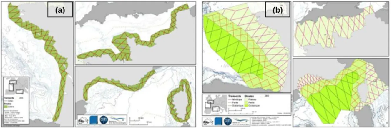
Transects followed a zigzag pattern as this optimizes the use of available flight time by reducing transit while providing a uniform coverage of the area. Transects were equally distributed and oriented in order to sample the different depths across all bathymetric strata (Fig.7).
Fig. 7. – Sampling design: transects planned in (a) coastal stratum; (b) neritic, slope and oceanic strata (from light green to dark green) (Pettex et al., 2012). Effort actually flown may differ in some areas because of field conditions, notably wind regime (Appendix B).
2.3.3 Data organization
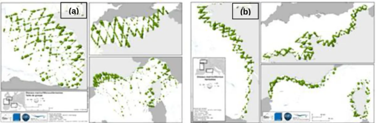
Transects were organized in legs of identical detection condition and further split into segments of 10 km, to avoid excessive variability in observation conditions (see Appendix B for transects flown per month during the two surveys). Moreover, segments with poor observation conditions, i.e. all segments with sea state Beaufort ≥4 and poor subjective observation conditions were removed. Finally, the software ArcGis 10 (ESRI, 2011) was used to locate on a map the sightings of each species groups and join observations to segments (Fig.8).
(a) (b)
Fig. 8. – Example distribution map of all seabird sightings throughout the study area in summer: (a) neritic, slope and oceanic strata; (b) coastal stratum (Pettex et al., 2012).
2.4 Habitat variables
Oceanographic and physiographic variables were selected to model seabird habitats (Table 2; see also Appendix D for variables which were tested but not included in models). Table 2. – Environmental variables used to model seabird habitats.
Physiographic Covariates Sources
Slope Slope (degree) GEBCO 2008
Depth Depth (m) GEBCO 2008
Dc Distance to the nearest coast (km) QGIS 2.2.0
DRC Distance to the nearest rocky coast (m) QGIS 2.2.0 DSC Distance to the nearest sandy coast (m) QGIS 2.2.0 Dcolony Distance to the nearest seabird colony (m) QGIS 2.2.0
Oceanographic covariates
SSTM Average sea surface temperature (K) ODYSSEA model SSTV Variance of sea surface temperature (K) ODYSSEA model SSTgrad Gradient of sea surface temperature (K) ODYSSEA model
SSHM Average sea surface height (m) MARS 3D/INGV models
SSHsd Standard deviation of the sea surface height (m) MARS 3D/INGV models Currents Daily maximum intensity of the currents (m.s-1) MARS 2D model
Physiographic variables (slope and depth) were obtained from the GEBCO 30 sec grid
(General Physiographic Chart of the Ocean; http://www.gebco.net/). This grid was also used in QGIS-2.2.0-Valmiera (QGIS Development Team, 2014), to calculate distance to nearest colony (Dcolony) and distance to nearest coast (Dcoast). They represent the shortest distance
between midpoint of each segment and the location of a colony or the 0 m isobath. Distance to nearest sandy coast (Dsandy coast) and nearest rocky coast (Drocky coast) were also calculated
thanks to the Eurosion database (Geology, Geomorphology and Erosion Trend; www.eea.europa.eu/data-and-maps/data/shoreline). Distance to colony was included in the models only for the summer season, as it is the breeding season for most seabird species: however breeding seasons (Appendix A) generally do not fully match our summer survey period. Colony locations were summarized from Cadiou et al., (2005) for France, JNCC
(Joint Nature Conservation Committee; www.jncc.defra.gov.uk) for United-Kingdom and SEO/BirdLife (www.seo.org) for Spain (Appendix C showed referenced colonies).
Daily sea surface temperatures (SST) were extracted from ODYSSEA model
(IFREMER; http://www.myocean.eu/) and then, averages and variances were calculated for each sampled days during the surveys with a temporal resolution of 7 and 28 days. We also computed SST gradients as the difference between the minimum and maximum SST values found in the eight pixels surrounding any given pixel (Fig.9); temporal resolutions of 7 and 28 days were used.
Fig. 9. – Calculation of SST gradients.
In addition, we used data extracted from models provided by Previmer
(www.previmer.org). Thanks to the MARS 3D model (Previmer, 2014), we were able to extract the daily sea surface height (SSH) (0.05° spatial resolution) for the two survey seasons and then calculate its average and standard deviation for the 7 and 28 days prior to sampled day.
Data of MARS 2D model provided by Previmer (www.previmer.org), allowed us to extract the hourly speed of tidal currents in the Atlantic Ocean for the survey periods. Thus, we could calculate maximum intensity of tidal currents with a resolution of 7 and 28 days.
Finally, we created a joint between the centre of each segment and habitat variables to assign the values of all variables to the location of each segment and date of the surveys (Appendix E showed average contribution of each environmental covariate).
2.5 Model construction
2.5.1 Model development
To model relationships between seabird distributions and environmental variables and to predict seabird distributions, we used GAMs (Hastie and Tibshirani, 1986) which permit to identify correlations between the number of animals and a variety of habitat parameters. This method takes into account the non-Gaussian distribution of individuals and non-linear dynamics of marine habitats and allows maximizing the quality of inference, description and prediction of habitats.
In the present study, we modelled the response variable Y (number of individuals per segment) with a link function g() which relates the mean of the response variable μ=E(Y|X1,...,Xn) to the additive predictor
as:
where
are non-parametric smooth functions (splines) of the covariates (Hastie and Tibshirani, 1986). Accounting for non-constant effort, we included an offset which takes into account the variation in the amount of effort per segment and was calculated as segment length multiplied by twice transects width (2*200 m). We tested the effect of oceanographic and physiographic covariates on abundance for each season and each seabird group by using quasi-Poisson distribution with variance proportional to the average to avoid over-dispersion of tail distributions (Hedley et al., 1999). A logarithmic link function was used to relate the average of the response variable and the additive predictor. To avoid over-fitting of the data, which has no ecological averaging (Ferguson et al., 2006), we restricted curve smoothing to three degrees of freedom. GAMs were fitted in R-3.0.1 (R Core Team, 2013)
with themgcv package, especiallygamand predict.gamfunctions (Wood, 2006; 2013).
2.5.2 Model selection and predictions
For model selection, oceanographic and physiographic variables described in 2.3 were used. Correlations between variables were calculated and we excluded pairs of collinear variables (i.e. with a Spearman coefficient <-0.7 and >0.7 calculated with Hmisc package
(Harrel, 2013). For each seabird group, observation outliers and environmental variables outliers were excluded and all models with combinations of 1, 2, 3 or 4 covariates were tested.
The model with the lowest generalized cross-validation (GCV) associated to the highest explained deviance, which evaluate the model’s fit to the data, was selected. Following Mannocci et al. (2013), a maximum of four covariates per model was used to avoid excessive complexity of models and difficulty in their interpretation. Finally, from the predict function of the mgcv package (Wood, 2013), we wrote a script permitting to calculate the contribution of each covariate in the selected model.
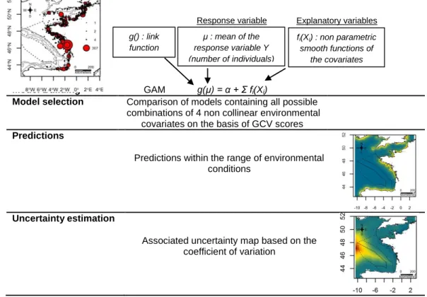
For each group of species, the best model and the associated covariates were used to predict relative density of individuals in a generated grid of 0.05° x 0.05° resolution. We first calculated daily predictions for all days of the surveys by using the predict function and then we calculated the average prediction over the entire period. We also computed an associated coefficient of variation (CV=sd/average) to provide uncertainty maps. Prediction grids include the sampled geographic sectors and extend outside of study area within the range of covariates used in model fitting to avoid extrapolation (Fig.10).
Model Building GAM g(μ) = α + Σ fi(Xi)
Model selection Comparison of models containing all possible combinations of 4 non collinear environmental
covariates on the basis of GCV scores
Predictions
Predictions within the range of environmental conditions
Uncertainty estimation
Associated uncertainty map based on the coefficient of variation
Fig. 10. – Stages of habitat modelling (example of herring gull complex in winter). Response variable μ : mean of the response variable Y (number of individuals) Explanatory variables g() : link function fi(Xi) : non parametric smooth functions of the covariates
2.6 Assessment of marine protected areas
To assess marine protected areas, we calculated a ratio to obtain a percentage of individuals included in the area compared to the total number of individuals predicted across the entire study area. To do this, we used files of all Special Protected Area (SPA) and Marine Nature Park (MNP) delimitations as well as offshore putative limits of proposed MPA (Fig.11). According to the “Birds Directive” (Directive 2009/147/CE, Parlement Européen, 2009), a protected area has to be designated when more than 1% of individuals present in a MS national EEZ are included in the area.
Thanks to the extract function from raster package (Hijmans et al., 2014), we extracted predicted densities for every pixel in all MPA and in the whole study area. Then we ranked all MPAs in term of seabird densities and determined the proportion of total abundance that is present in every MPA.
Fig. 11. – Marine Protected Areas used for the assessment (provided by MPA Agency).
3 Results
3.1 Data processing
3.1.1 Detection conditions and survey effort
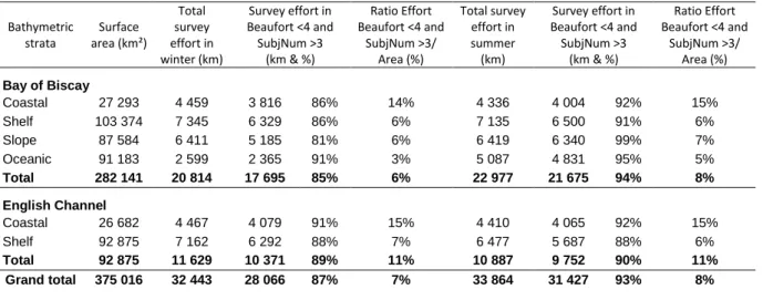
The aerial survey actually covered 32,445 km of transects in winter and 33,864 km in summer, which represent respectively 8.65% and 9.03% of the surface of the study area, given the 200 m sighting band on each side of the track (English Channel and Bay of Biscay) (Table 3). The focal species were mostly observed in the coastal and shelf strata, which correspond together to 72% of total effort. Detection conditions were very good during the two surveys with 87% of effort in winter and 93% of effort in summer carried out under sea state ≤ 4 and medium to excellent subjective conditions. Overall, detection conditions were a little better in the Bay of Biscay than in the Channel in the summer (94% of effort with sea state ≤ 4 versus 90%); conversely in winter, detection conditions were better in the Channel than in the Bay of Biscay (89% versus 85%).
For habitat analysis, we did not consider poor detection conditions (sea state ≥4 and subjective observation conditions poorer than medium) to ensure correct identification of species. Hence, effort considered for analysis spanned 28,068 km of transects in the winter (i.e.7% of the surface of the study area) and 31,427 km in the summer (i.e. 8% of the surface of the study area).
Table 3. – Effort by strata performed during the two surveys. This table presents the total effort carried out in the Bay of Biscay and the Channel in winter and summer and the effort used for analysis without taking into account poor observation conditions (Beaufort ≥4 and subjective observation (SubjNum) conditions poorer than medium).
Bathymetric strata Surface area (km²) Total survey effort in winter (km) Survey effort in Beaufort <4 and SubjNum >3 (km & %) Ratio Effort Beaufort <4 and SubjNum >3/ Area (%) Total survey effort in summer (km) Survey effort in Beaufort <4 and SubjNum >3 (km & %) Ratio Effort Beaufort <4 and SubjNum >3/ Area (%) Bay of Biscay Coastal 27 293 4 459 3 816 86% 14% 4 336 4 004 92% 15% Shelf 103 374 7 345 6 329 86% 6% 7 135 6 500 91% 6% Slope 87 584 6 411 5 185 81% 6% 6 419 6 340 99% 7% Oceanic 91 183 2 599 2 365 91% 3% 5 087 4 831 95% 5% Total 282 141 20 814 17 695 85% 6% 22 977 21 675 94% 8% English Channel Coastal 26 682 4 467 4 079 91% 15% 4 410 4 065 92% 15% Shelf 92 875 7 162 6 292 88% 7% 6 477 5 687 88% 6% Total 92 875 11 629 10 371 89% 11% 10 887 9 752 90% 11% Grand total 375 016 32 443 28 066 87% 7% 33 864 31 427 93% 8% 3.1.2 Seabird sightings
In the whole study area, a total of 18,155 sightings of seabirds were collected in winter and 8,439 in the summer (Appendix F). Among these sightings, our groups of coastal species represented 2,459 sightings in winter and 3,318 sightings in summer (Table 4, Appendix F). Irrespective of the season, black-backed gulls and herring gull complex were the most frequently encountered taxa whereas the least observed seabirds were terns in the winter and scoters in the summer (see Appendix F for seabird sightings during the two seasons).
Most of studied species were observed in coastal and neritic strata but in varying proportions (see Appendix G for sighting maps of each group). Individuals of the herring gull complex were more common in the summer than in winter in Channel/Bay of Biscay, with an encounter rate of 4.57 against 2.75 sightings.100km-1. Conversely, black-backed gulls were slightly more common in winter than in summer (2.70 sightings.100km-1 and 2.41 sightings.100km-1 respectively). Terns were much less frequently observed in winter (0.27 sightings.100km-1) than in summer (2.16 sightings.100km-1). Conversely, cormorants and shags were more observed in winter (0.77 sightings.100km-1) than in summer (0.58 sightings.100km-1). Divers were mainly observed in the Channel (99% of sightings) and only in winter with an encounter rate of 0.66 sightings.100km-1). Finally, scoters were hardly observed in summer (0.07 sightings.100km-1) and more frequent in winter (0,42 sightings.100km-1).
Table 4. – Number of sightings and individuals (Ind nb) in each group by sector and season. English Channel / Bay of Biscay
Groups Winter Summer
Sightings Ind nb Sightings Ind nb
herring gull complex 892 3133 1549 3367
black-backed gulls 877 2079 816 1420
terns 88 203 731 1437
cormorants and shags 250 555 198 493
divers 215 846
scoters 137 2086 24 94
Because of the absence of some species or of the small number of sightings combined with poor observation conditions, some habitat models were not feasible. Hence, models for divers and scoters in summer have not been fitted in the following section.