• Aucun résultat trouvé

Temperature, geometry, and bifurcations in the numerical modeling of the cardiac mechano-electric feedback.

N/A
N/A
Protected

Academic year: 2021

Partager "Temperature, geometry, and bifurcations in the numerical modeling of the cardiac mechano-electric feedback."

Copied!
13
0
0

Texte intégral

(1)

mechano-electric feedback

A. Collet, J. Bragard, and P. C. Dauby

Citation: Chaos 27, 093924 (2017); doi: 10.1063/1.5000710 View online: http://dx.doi.org/10.1063/1.5000710

View Table of Contents: http://aip.scitation.org/toc/cha/27/9

Published by the American Institute of Physics

Articles you may be interested in

Modeling dynamics in diseased cardiac tissue: Impact of model choice

Chaos: An Interdisciplinary Journal of Nonlinear Science 27, 093909 (2017); 10.1063/1.4999605

Effects of mechanical feedback on the stability of cardiac scroll waves: A bidomain electro-mechanical simulation study

Chaos: An Interdisciplinary Journal of Nonlinear Science 27, 093905 (2017); 10.1063/1.4999465

Suppression of turbulence by heterogeneities in a cardiac model with fiber rotation

Chaos: An Interdisciplinary Journal of Nonlinear Science 27, 093921 (2017); 10.1063/1.5000225

Nonlinear diffusion and thermo-electric coupling in a two-variable model of cardiac action potential

Chaos: An Interdisciplinary Journal of Nonlinear Science 27, 093919 (2017); 10.1063/1.4999610

Fast-slow asymptotic for semi-analytical ignition criteria in FitzHugh-Nagumo system

Chaos: An Interdisciplinary Journal of Nonlinear Science 27, 093916 (2017); 10.1063/1.4999472

Modeling bipolar stimulation of cardiac tissue

(2)

Temperature, geometry, and bifurcations in the numerical modeling

of the cardiac mechano-electric feedback

A.Collet,1J.Bragard,2and P. C.Dauby1,a)

1

GIGA In silico medicine, Lie`ge University, B-4000 Lie`ge, Belgium 2

Physics and Applied Math. Dept., Universidad de Navarra, Pamplona E-31080, Spain

(Received 31 March 2017; accepted 17 August 2017; published online 31 August 2017)

This article characterizes the cardiac autonomous electrical activity induced by the mechanical deformations in the cardiac tissue through the mechano-electric feedback. A simplified and qualita-tive model is used to describe the system and we also account for temperature effects. The analysis emphasizes a very rich dynamics for the system, with periodic solutions, alternans, chaotic behav-iors, etc. The possibility of self-sustained oscillations is analyzed in detail, particularly in terms of the values of important parameters such as the dimension of the system and the importance of the stretch-activated currents. It is also shown that high temperatures notably increase the parameter ranges for which self-sustained oscillations are observed and that several attractors can appear, depending on the location of the initial excitation of the system. Finally, the instability mechanisms by which the periodic solutions are destabilized have been studied by a Floquet analysis, which has revealed period-doubling phenomena and transient intermittencies.Published by AIP Publishing. [http://dx.doi.org/10.1063/1.5000710]

Myocyte contraction is generated by an electrical signal (action potential) that orchestrates the synchronization of the cardiac tissue. The resulting deformation of the car-diac myocytes influences the electrical characteristic of the heart. This two-way coupling can induce auto-oscillations in the system. In our work, this autonomous activity is studied in terms of the temperature of the heart and also in terms of the size of the system and of the importance of the electro-mechanical coupling. In particular, we show that bifurcations can occur that destabilize the auto-oscillations and give rise to period-doubling phenomena and transient intermittencies.

I. INTRODUCTION

The modelization of the heart dynamics poses outstand-ing challenges. The heart modeloutstand-ing combines fluid, mechani-cal, and electrical descriptions. To date, very few numerical simulations have been able to combine those effects in a sin-gle model and as an exception we can cite the remarkable multiphysics model of Watanabeet al.1Indeed, the cardiac muscle involves sub-cellular and cellular processes (e.g., actin-myosin interaction) as well as mechanisms at the tissue level [e.g., propagation of action potentials (APs)]. Large scale and small scale processes are strongly intertwined. Microscopic phenomena at the sub-cellular level will modify the macroscopic properties at the tissue level and vice-versa.2

However, simplified models have brought a great deal of knowledge to the field of cardiac dynamics. It is now well established that cardiac arrhythmias are characterized by an incorrect propagation of the electrical action potentials.3

These arrhythmias may in some cases degenerate through instabilities into the formation of spiral or scroll waves and lead to life threatening situations.4–6 In most cases, studies are done by neglecting the excitation-contraction coupling that is present inside the heart.

Our work is mainly focused on the macroscopic electro-mechanical behavior of the heart. We will in fact extend the ideas put forward in a paper by Alvarez–Lacalle and Echebarria,7where a simple model is used to study the influ-ence of the cardiac contraction on the stability of the action potentials. Let us emphasize that our basic model is the same as that proposed in Ref.7, but our deduction of the equations is different and corrects several inaccuracies. Note also that in addition to the coupling between electrical and mechani-cal phenomena which was considered in Ref. 7, we also include the effects of temperature variations on the electrical activity and the electromechanical behavior.

Temperature variations affect the cardiac dynamics. One can cite, for example, the known relationship between the sud-den cardiac death related to the Brugada syndrome and the increase in patient body temperature.8The study of tempera-ture effects is also important because of the more common usage of hypothermia in medical settings. Hypothermia has been shown to be a beneficial effect in resuscitation therapy. Recent modeling studies9,10have put forward that fibrillation is dependent on the system size and the body temperature. These studies claim that fibrillation tends to be easier to initi-ate at lower temperatures and that the frequency of fibrillation decreases with lower temperatures.

The mechano-electric feedback (MEF) is the influence of mechanical deformations on the electrical behavior of the heart. This phenomenon has been studied for a long time, both experimentally and theoretically (see for instance Refs.7and 11–22) and it is now well accepted that MEF can elicit sponta-neous oscillatory behavior in muscle fibers. In the present a)

pc.dauby@ulg.ac.be

(3)

work, we propose a theoretical and numerical analysis of such oscillations. Our approach is based on a general and qualita-tive model of the system which takes into account and com-bines all the fundamental basic phenomena at work in these oscillations. The model is developed from basic principles and appropriate assumptions, before being used to describe the bifurcation phenomena that can destabilize these oscillations.

We will also emphasize geometrical effects and analyze the influence of the position of the pacemaker that generates these oscillations.

The other main objective of this work is to study the influence of the temperature on the self-sustained oscillations that appear in an electromechanical model of the cardiac tis-sue. We will confirm that temperature is indeed an important parameter for the stability of such oscillatory behavior and that the frequency of self-sustained oscillations decreases together with the temperature. We will supplement the numerical computation by a mathematical analysis that con-firms the numerical results.

This paper is organized as follows. In Sec.II, we present the equations that govern the dynamics of the heart muscle. In particular, we take into account the thermo-electro-mechanical (TEM) effects that are taking place in the cardiac tissue. We then reduce the general model to a simplified one-dimensional globally coupled model. In Sec.III, we analyze the results obtained by the simplified model. In particular, we study the influence of the temperature on the appearance of the self-sustained dynamics in the system. We also con-sider thoroughly the geometrical effect of the location of the initial excitation on the subsequent dynamics. We conclude Sec.IIIby a theoretical study of the stability of the periodic solutions using the Floquet theory. In Sec.IV, we conclude the paper and discuss future possible extensions of this study.

II. MODEL AND METHODS

A. Governing equations

In the present section, we introduce a general time-dependent thermo-electro-mechanical (TEM) model of the heart muscle. The equations introduced below must be con-sidered as a qualitative model of the heart, taking into account the propagation of action potential, the electro-mechanic feedback, and the influence of temperature, thus allowing the study of the many couplings between these dif-ferent phenomena. In our approach, we will assume that the propagation of action potential is governed by a standard monodomain equation.23,24 If V is the dimensionless mem-brane potential, this equation can be written as

@ V @t ¼ D 0 @ @XM JðC 1ÞMN @ V @XN    iion iapp; (1)

where D0 is a diffusion coefficient often taken equal to 1 cm2s1.7 The

XM are the material coordinates and the matrix of contravariant components ðC1ÞMN

is the inverse of matrixCMNdefining the right Cauchy-Green deformation

tensor C (boldface symbols are used to indicate tensorial quantities). The symbolJ denotes the volume ratio (ratio of

the deformed to the undeformed volume element). Finally, the quantityiion describes the ionic currents through the cell

membrane, while iapp accounts for a possible externally

applied current (these currents are here expressed in s1). Note that the boundaries of the spatial domain are assumed electrically insulating and we will thus use Neumann bound-ary conditions in the numerical computations.

Considering the Nash-Panfilov monodomain model,20,21,25 the ionic current term can be written as

iion¼ iionðV ; v; i sacÞ ¼ jvV ðV 1Þ ðV aÞ þ V vþ isac;

(2) where jvanda are model parameters related to the

excitabil-ity properties of the system, while v and isac are quantities

whose meaning is described now. First, v is a recovery gate variable whose dynamics in the Nash-Panfilov model is gov-erned by the following equation:

dv

dt¼ e ð Þ jV ð vV vÞ : (3) In this equation, parameter jvallows controlling the

ampli-tude of the recovery variable v, while eð VÞ describes the time delay between the variations of the recovery variable and those of the transmembrane potential. Following Ref. 21, this function is assumed to be piecewise constant and equal to either e0 or e1 depending on V being, respectively,

larger or smaller thana.

Let us now describe the mechano-electric feedback (MEF) and the associated stretch-activated current (SAC) isac, which represents the contribution to ionic currents

resulting from the stretching of the myocardial cells. Detailed models of stretch activated currents (SACs) can be found in the literature (see for instance Refs. 14, 17, and 19). However, since our approach is first qualitative and interested in physical mechanisms, we will instead of well accepted but rather complex models use a very simple and generic description of the SACs, inspired by Ref. 22 and also used in Ref. 7 and 20. If k denotes the ratio of the lengths of the stretched and relaxed sarcomeres, we will express the stretch activated current as

isac ¼ gsacðV esacÞ k  1ð Þ H k  1ð Þ ; (4)

where gsac and esac describe the conductance and reversal

potential of the stretch-activated channels (following Refs. 20 and21, we will setesac¼ 1), while H denotes the

stan-dard Heaviside step function. This expression simply describes a linear increase of the current with the stretch-ing and also assumes that no current is present when the sarcomere is compressed. Let us mention that in Refs. 7, 20, and 22, k in the above formula is replaced by the deformed to undeformed volume ratio, which is a bit spe-cious since these authors also use deformation energies corresponding to incompressible materials, for which this ratio is 1.

If external body forces are not taken into account and if a quasi-static equilibrium is assumed, mechanics is described by the following equation:

(4)

0¼ FmNS MN


jM; (5)

where SMN is the second Piola-Kirchhoff stress tensor and FmNis the deformation gradient tensor, with indicesm and N

corresponding to, respectively, spatial and material coordi-nates. Notation jM indicates a covariant derivative with

respect toXM.

Contraction and deformation of muscle tissue involve both passive and active behaviors and several approaches are possible to analyze this problem. Interesting, but rather com-plex descriptions based on active strains and thermodynam-ics have been proposed for instance in Refs.26–29. Here, we will instead consider the active stress approach, which amounts to simply assume that the stress tensor can be expressed as a linear superposition of an elastic contribution SMN

elastic, describing the passive properties of cardiac tissue,

and an active part SMN

active, resulting from the contractile

behavior of the muscle SMN¼ SMN

elasticþ S MN

active: (6)

The elastic contributionSMN

elastic is obtained by considering a

compressible isotropic hyperelastic material and a Mooney-Rivlin model30,31and one gets

SMNelastic¼ 2 c1GMNþ 2 c2 tr C GMN GMOGNPCOP


J d ðC1ÞMN; (7)

where c1, c2, and d are elastic material constants,

tr C¼ GOPC

OP, whileGMNare the contravariant components

of the metric tensor.32To introduce the constitutive equation for the active part of the stress tensor, we will consider first the Cauchy stress tensor instead of the second Piola-Kirchhoff. Indeed, the Cauchy stress tensor describes the actual stress on the deformed configuration and can thus more naturally be related to the cascade of phenomena link-ing the electrophysiology to the contraction in the myocar-dium. Under the simplifying assumption of isotropy, the active tension can be accounted for by a scalar quantity that will be denoted as ractive, and the active Cauchy stress tensor

ractive will be simply expressed as the product of this scalar

by the metric tensor g in the current configuration

ractive¼ ractiveg : (8)

This relationship can then be expressed in terms of second Piola Kirchhoff stress tensor and one gets

SMNactive¼ J ractiveðC1Þ MN

: (9)

As already mentioned earlier, contraction in a muscle cell results from a cascade of phenomena involving many actors, such as action potential propagation, calcium ion flows, myosin dynamics, etc. In our qualitative approach, we will simply describe this whole cascade of phenomena by assuming that the generated scalar tension ractive is directly

related to the membrane potential, which is the very first cause of all phenomena. Considering that the active tension is driven by the variations of the membrane potential, the fol-lowing evolution equation for ractivewill be postulated7,25,33

dractive

dt ¼ e ð Þ jV ractiveV ractive


; (10)

where jractive is a parameter that controls the amplitude of the active stress twitch and eð VÞ, already introduced above, accounts for the delay in the development and recovery of the active tension with respect to the action potential.

In order to take into account the influence of temperature in the system, we introduce two temperature-dependent func-tions mimicking the thermo-electric coupling in the electro-mechanical model. First, the gating kinetics of ion channels is assumed to be temperature-dependent via temperature-dependent rates for the conformational transitions of the subu-nits constituting the ion channels. Assuming an exponential dependence, the r.h.s. of Eq.(3)is multiplied by the following nonlinear temperature-dependent function:34,35

u Tð Þ ¼ Q TT0

10

10 ; (11)

where T is the absolute temperature, T0is a reference

tem-perature, andQ10represents the well-known 10-degree

tem-perature coefficient that measures the change of rates due to a temperature increase of ten degrees.36,37 Furthermore, since the evolution equation (10), which describes the dynamics of the active tension development, can also be con-sidered as a biochemical process, the influence of tempera-ture on this equation can be accounted for by multiplying the r.h.s. of (10) by the same function uðTÞ which was intro-duced in the modeling of the gating kinetics of ion channels.

The second temperature-dependent function is intro-duced to model the changes in ionic conductances when the temperature is not constant. If the conductances are assumed to vary linearly,34,35the ionic currents(2)are multiplied by

g Tð Þ ¼ 1 þ B T  Tð 0Þ ; (12)

where B is a constant parameter that describes the rate of change of conductance with temperature. In the following, one will take T0¼ 37C and the two parameters Q10 andB

will be fixed to values whose orders of magnitude corre-spond to values from the literature10,34,35 Q10 ¼ 3 and

B¼ 0:008 K1.

B. 1-D model and global coupling

Even if the thermo-electrico-mechanical model devel-oped above was kept as simple as possible, it involves many physical phenomena of different origins and is thus rather complex. Indeed electrical and mechanical phenomena inter-play in a bidirectional way, via the excitation-contraction coupling (ECC) and the MEF, while electrical and thermal phenomena are coupled in a unidirectional fashion. In this context, the role played by the MEF in the TEM behavior of the cardiac muscle tissue and the underlying fundamental mechanisms are not easy to characterize. In order to avoid additional complexities related to the geometry and to con-centrate on the physical mechanisms, we will in the follow-ing consider a one-dimensional situation, correspondfollow-ing to an idealized one-dimensional cardiac fiber.

(5)

In the case of the 1-D fiber, the gradient deformation tensor, F, and the right Cauchy–Green deformation tensor, C, are reduced to single scalar quantities

F¼ F1 1¼ @x @X (13) and C¼ C11¼ F2: (14)

In Eq.(13),x and X are, respectively, spatial and material Cartesian coordinates along the cardiac fiber. Note also that the local stretching k is identical to F, and the trace and the determinant of the right Cauchy–Green deforma-tion tensor are reduced toF2. The stress tensors also reduce to scalars and from (7), the only relevant component S11

elastic, more simply denoted as Selastic, of the passive part

of the second Piola-Kirchhoff stress tensor, Selastic, can be

written as

Selastic¼ 2 c1

d

F: (15)

Let us now define the reference configuration of the fiber as the state where no active tension is present and where no extension or contraction of the fiber is imposed. In this situa-tion, the fiber has its natural length and we will assume that the (total) stress in the fiber is then equal to zero. Since the total stress is equal to the elastic contribution in the reference configuration, and since this configuration is characterized byF¼ 1, one deduces from the equation above that d ¼ 2c1,

which allows writing

Selastic¼ d 1 

1 F


: (16)

From (9), one also deduces that Sactive¼ S11active¼

JractiveðC1Þ 11

¼ Jractive=C11 ¼ ractive=F and the unique

rel-evant component S¼ S11 of the total stress tensor is given

by S¼ d 1 1 F   þractive F : (17) Then,(5)becomes @ F Sð Þ @X ¼ 0 ; (18)

andF S is constant with respect to X. Introducing the nota-tionF S¼ A ¼ AðtÞ, and solving(17)with respect toF, one obtains

F¼ 1 þ1

dðA ractiveÞ : (19) Considering that both ends of the 1-D fiber of lengthL are held fixed, one has

ðL 0

F Xð Þ dX ¼ L : (20)

Introducing (19) in this relationship provides A¼ ractive,

where ractive is the mean value of ractive over the fiber.

Equation(19)can thus be rewritten as F¼ 1 þ1

dðractive ractiveÞ : (21) This relationship emphasizes what Alvarez et al.7called a “global coupling” in the system, the latter being character-ized by the influence of the mean active tension (a global notion) on the local stretching k¼ F.

Introducing expression (21) of F¼ k in (4) allows rewriting the SACs in terms of ractiveand one has

isac¼

gsac

d ðV 1Þ rð active ractiveÞ H ðractive ractiveÞ: (22) From (3) and (10), it can be seen that v=jv and

ractive=jractive obey the same ordinary differential equation (ODE). Assuming similar initial conditions for v=jv and

ractive=jractive, the following algebraic relationship between ractiveand v is then found

ractive¼

jractive jv

v : (23)

Thus, Eq.(22)can be rewritten as

isac¼ ~gsacðV 1Þ v  vð Þ H v  vð Þ ; (24)

with v the mean value of v and ~ gsac ¼ gsac d jractive jv : (25)

In the one-dimensional problem, the first term of the r.h.s. of(1)can be written as D @ @X 1 F @ V @X   : (26)

In the following, we will also assume that deformations remain small, which allows writing F¼ 1 þ d, with d  1. Then, the diffusive term(26)can be developed in series of d and all but the leading term can be neglected, which amounts to approximating the above expression byD @2V =@X 2. (Note

also that it was checked numerically in Ref. 38 that this approximation is indeed quite good.) The whole set of equa-tions that govern the 1-D thermo-electro-mechanical prob-lem is then made up of the evolution equations of the membrane potential and the relationships describing the influence of temperature. The former equations take the form

@ V @t ¼ D @2V @X2 f ðV ; v; isacÞ g Tð Þ  iapp; (27) dv dt¼ e ð Þ jV ð vV vÞ u Tð Þ ; (28) with f ðV ; v; isacÞ ¼ jvV ðV 1Þ ðV aÞ þ V vþ isac; (29)

(6)

isac¼ ~gsacðV 1Þ v  vð ÞH v  vð Þ; (30)

e ð Þ ¼ eV 0H ðV aÞ þ e1H að  VÞ: (31)

The influence of temperature is described by the following relationships: g Tð Þ ¼ 1 þ B T  Tð 0Þ; (32) u Tð Þ ¼ Q TT0 10 10 : (33)

In this globally coupled model, the mechanical proper-ties do not appear explicitly but their influence is taken into account by the specific form of the SACs. Note also that, except for the temperature dependence, these equations are the same as those presented in Ref.7. However, the deduc-tion is different here and in particular,, fewer hypotheses are necessary to deduce the global coupling.

The main purpose of the paper is the study of the set of Eqs. (27)–(33). In the following, these equations will be solved numerically and the behavior of the solutions as a function of important parameters will be analyzed in detail.

C. Numerical techniques

The set of Eqs. (27)–(33) must be solved numerically and we describe briefly now the method used in this paper. The spatial discretization of the cardiac fiber is done on a regular mesh where the spatial grid is fixed to DX¼ 0:02 cm.39The Laplacian is discretized using a standard second-order central difference scheme and the spatial average (denoted by an over-bar) in Eqs.(27)–(33)is computed using Simpson’s rule.40 For the temporal integration of Eq. (27), we have used the explicit Runge–Kutta method. In particu-lar, we have used the fifth order Cash–Karp Runge–Kutta method.41 This high order method is suitable for the initial value problem having rapidly varying solutions as is the case in the present problem. A time step of Dt¼ 0:04 ms has been chosen here and it has been checked to be sufficiently small to give accurate results independent of the time step. Note that we have also checked that the spatial grid is suffi-ciently small to get consistent results. Indeed, using DX¼ 0:01 cm gives essentially the same results. The boundary conditions imposed on the membrane potential V at the extremities of the fiberX¼ 0 and X ¼ L is @XV¼ 0 and they

correspond to boundaries in contact with an electrical insula-tor. For the initial condition of Eq.(27), an external current, iapp, is applied locally on a small region, which has a 5 DX

extension, and during a time interval of 5 ms. The amplitude of the imposed stimulation current is set toiapp¼ 0:06 ms1.

III. RESULTS

A. Autonomous electrical activity (AEA)

In normal physiological conditions, the mechanical feedback ensures the stability of the action potential propa-gation. However, in pathological situations the coupling between the electrical and mechanical parts of the cardiac dynamics may lead to sustained oscillations even without an external pacemaker. These self-sustained oscillations define

an autonomous electrical activity (AEA) of the heart, which is illustrated in Fig. 1. The values of the parameters that were used to obtain this figure are those given in Table I, with L¼ 5 cm, ~gsac¼ 0:05, and T ¼ 37C. In the situation

described by the figure, the action potential is initiated at

the lower end of the fiber (symmetrically around

X¼ 0.5 cm) by injecting the external current iapp into the

system. From this location, two waves are then elicited. One wave is moving downwards and is rapidly eliminated by hitting the lower boundary of the fiber. The wave going up towards the boundary at X¼ 5 cm is first propagating at a rather constant speed. The passage of the action potential generates local shortening of the tissue. Due to the fact that the fiber length is constant other locations of the fiber are concomitantly stretched and SACs are generated. These SACs have two important effects. First, when the action potential is reaching approximately X¼ 4 cm, the SACs that have been accumulating in the higher end of the fiber are such that they generate a quasi instantaneous action potential in the region from X¼ 4 to X ¼ 5 cm. This phe-nomenon, that looks like a quasi infinite speed propagation, is a consequence of the global coupling in the system. Indeed, the length of the fiber being constant, contraction somewhere in the system generates stretching, and thus SACs, in all other parts of the fiber.

FIG. 1. Space-time plot of the action potential showing perpetual AEA on the cardiac fiber forT¼ 37C,L¼ 5 cm, and ~g

sac¼ 0:05 (cf. symbol þ in Fig.2). The color-coding quantifies the values of the dimensionless mem-brane potential V (color bar).

TABLE I. Parameter values used for the simulations of the one-dimensional model described by Eqs. (27)–(33).

Parameter Value Units

a 0.05 Dimensionless D0 103 cm2ms1 e0 3 103 ms1 e1 90 103 ms1 jractive 0.5 N cm 2 jv 2 ms1 ~ gsac ½0  0:12 Dimensionless d 1.6 N cm2 T0 37 C B 0.008 K1 Q10 3 Dimensionless L ½2  14 cm

(7)

Second, this action potential in the region between X¼ 4 cm to X ¼ 5 cm will in turn generate important stretch-ing in the lower end of the fiber and as a consequence a large release of SACs. These SACs, resulting again from the global coupling, are responsible for the triggering of a new action potential at the lower end of the fiber and the cycle can continue in a perpetual fashion. We observe the AEA in Fig.1for as long as the numerical simulation is continued.

The SACs are of course responsible for the AEA described before. In our model, the intensity of these currents is proportional to ~gsac, which is thus an important parameter.

Moreover, to generate these currents, stretching of the fiber is necessary, which is only possible if the length L of the fiber is controlled in some way. Here, we maintain a constant value to this length and the intensity of stretching will thus directly depend on this quantity. As far as the AEA is con-cerned, the two quantities ~gsacandL are thus the most

impor-tant parameters of our model and we will analyze in detail their influence on the self-sustained oscillations.

For this purpose, the ðL; ~gsacÞ parameter space is

scanned in a systematic way in order to determine the values of these parameters for which the AEA is sustained indefi-nitely. The values of the other parameters of the model are those given in TableI and the temperature is set to 37C. The initial excitation is applied to the region of the fiber ranging from L=10 0:04 cm to L=10 þ 0:04 cm. As indi-cated in Table I, the analysis is carried out for L ranging from 2 cm to 14 cm and ~gsac ranging from 0 to 0.12 with

increment steps of DL¼ 0:04 cm and D~gsac¼ 0:0005,

respectively. As a result, 72 000 numerical simulations have been performed to scan all the ðL; ~gsacÞ parameter space.

Note also that since the solutions of our equations can only be obtained numerically, we need to introduce an (arbitrary) practical definition of the permanency of a sustained oscilla-tion. In the following, we will consider the AEA as “perpetual” if it lasts at least 200 s. Of course, this does not mean that “transient” oscillations, lasting less than 200 s in a real patient’s heart, could not be life-threatening phenomena. The results are presented in Fig.2, where a color-plot of the duration of the AEA in terms ofL (horizontal axis) and ~

gsac (vertical axis) is given. The central area (CA) (red

online) in Fig. 2 corresponds to regions where the AEA is sustained indefinitely. This area is surrounded by (blue online) regions in which self-sustained oscillations cannot be triggered, even for a short time interval and by regions in which the AEA is sustained for a finite time interval (all other colored regions). The transitions between the regions in which the AEA is indefinitely sustained and those in which the AEA does not occur at all are quite sharp on the left and lower boundaries of the CA. On these boundaries, the disappearance of the self-sustained oscillations can be explained as follows.

For values ofL smaller than those corresponding to the left boundary of the main CA, the APD is too long to enable the SACs to generate an AP. After the propagation of the first AP due to the initial excitation, all the fiber is in a refractory state and therefore, even if the SACs are very large (large value of ~gsac), the electrical activity ends. For

values of ~gsac smaller than those corresponding to the lower

boundary of the main CA, SACs are not large enough to trig-ger a new AP after the propagation of the first one induced by initial excitation applied to the fiber. Thus, no AEA occurs in this region.

For the upper boundary of the CA, the transitions are dif-ferent. These transitions are from a perpetual AEA to finite AEA. Later, the Floquet stability analysis, conducted in Sec. III D, will corroborate that the transitions at the lower and upper boundaries of the CA are actually intrinsically different. Note also that above the CA, some “islands” exist, which cor-respond to sustained oscillations of finite or infinite duration.

Figure1has already shown an illustration of the typical spatio-temporal behavior of the system when the parameters ðL; ~gsacÞ remain within the CA, not ’too’ close to the

bound-aries. In this situation, this representation reveals that the AEA behaves in a periodic way with period-1 cycles. However, several examples show that the very rich dynamics of the system is not limited to such a rather simple behavior.

Figure3describes the space–time behavior correspond-ing to an “island” above the main CA (~gsac¼ 0:0745 and

L¼ 3:2 cm). For these values of the parameters, the AEA is still indefinitely sustained and periodic, but it takes the form of a period-11 cycle. Note however that by slightly modify-ing the value of ~gsac, and keeping constant the values of other

FIG. 2. Map of the persistence of the AEA induced by the MEF as a func-tion of the parameterL and ~gsacatT¼ 37C. The color scale ranges from 0 to 200 s. Note that the symbolsþ and  indicate the parameters correspond-ing to Figs.1and3, respectively.

FIG. 3. Space–time plot of the dimensionless membrane potential, V , for L¼ 3:2 cm and ~gsac¼ 0:0745, and with T ¼ 37C (cf. symbol * in Fig.2). Note that the time units (horizontal axis) are in seconds.

(8)

parameters, the AEA disappears. It is also interesting to ana-lyse the transient behavior that can sometimes take place before the oscillations vanish. As an example, consider the time evolution of the fiber whenL¼ 12 cm; ~gsac¼ 0:21, and

with T¼ 37C. For these values of the parameters, the

stretch-activated current isac is too strong and the dynamics

becomes unstable. However, Fig.4shows that a few oscilla-tions are generated after the first imposed activation but no periodic dynamics is ever reached and the system eventually tends to rest. In Fig.4(a), the initial excitation is located at the lower end of the system and in Fig.4(b), the initial excitation is shifted one grid point up with respect to the previous case of Fig.4(a). This very small difference between the location of the initial excitation becomes visible in the space–time plots in Fig.4after approximately 1.5 s. Figure 4thus illus-trates the transient space-time chaotic dynamics that is present for large values of the ~gsac parameter. This last result is in

agreement with one of the conclusions of the paper by Gizzi et al.42There the authors stated that the complex spatiotempo-ral patterns observed during alternans are very sensitive to both the site of stimulation and the stimulation history.42

In Secs.III B–III D, we examine how the AEA is influ-enced by temperature variations and also by changing the location of the initial excitation imposed to the fiber. Finally, we develop a Floquet analysis which will provide a much deeper insight into the disappearance of the AEA at the boundaries of the CA.

B. Influence of the temperature on the AEA

We describe now how temperature variations modify the behavior of the system. Before considering a thorough explora-tion of the (L, ~gsac) parameter space we can get some

quantita-tive insight of the influence of the temperature on the AEA by fixingL¼ 5 cm and ~gsac¼ 0:037 and computing

characteris-tics of the periodic oscillations. In Fig.5, we have displayed the period of the oscillation Tp (in ms), the action potential

durationAPD80 (in ms), and the wave speedc (cm s –1

) as a function of the temperature. The measurements are dependent on the location on the fiber (especially forc) and we have cho-sen to measure at the middle of the fiber, i.e.,X¼ 2.5 cm where the boundary effects are the least pronounced. The wave veloc-ity (black dashed line) in Fig.5has larger measurement errors and we compute the mean wave speed for 20 oscillations after a transient time of 40 s has elapsed. The standard deviations for the wave speed are also displayed as error bars in Fig.5. As the temperature is increased the wave speed increases sub-stantially (vertical axis on the right-hand-side of Fig.5).

The oscillation periodsTp(red solid line in Fig.5) and

the action potential duration APD80 (green dotted-dashed

line in Fig.5) follow the same trend (vertical axis on the left-hand-side of Fig.5). An increase of the temperature leads to shorter periods and shorter action potentials. Here again, we have averaged the measurements on 20 oscillations after a long transient time (40 s) has elapsed. The standard devia-tions forTpandAPD80are not shown in Fig.5because they

are too small to be noticeable.

Let us now turn to the effect of temperature on the AEA regions in the (L, ~gsac) parameter space. In particular, we are

interested in showing if the size of the regions where oscilla-tions are indefinitely sustained (CA) varies with temperature. The results are displayed in Fig.6, which provides the same information as Fig.2, but for values of the temperature fixed to 33C; 35C; 39C, and 41C. By analyzing panels (a) to (d) in Fig. 6, and also Fig.2, we observe that i) the area in the ðL; ~gsacÞ space where the AEA is indefinitely sustained

becomes larger when the temperature is increased; ii) the left boundary of the main CA is shifted to a smaller system size when the temperature is increased; iii) the number of islands of the AEA for large values of the ~gsacis increased at higher

temperature; iv) the lower and upper boundaries of the main CA are steeper for higher temperature.

C. Effect of the location of the initial excitation

1. Different dynamical attractors

Another important parameter of the dynamics of the sys-tem governed by Eqs.(27)–(33)is linked to the location of FIG. 4. Space–time plot of the dimen-sionless membrane potential, V , for L¼ 12 cm and ~gsac¼ 0:21, and with T¼ 37C. The upper graph (a) corre-sponds to an initial excitation at the lower endX¼ 0, the lower graph (b) corresponds to an initial excitation shifted up by one grid point with respect to case (a).

FIG. 5. Variation of the periodTp (red solid line),APD80 (green dotted-dashed line), and wave speedc (black dashed line) measured at the middle of the fiber as a function of temperature. Here,L¼ 5 cm and ~gsac¼ 0:037 are fixed.

(9)

the initial excitation in the cardiac fiber. In this section, we illustrate the difference of behavior of the system when one modifies the location of the initial condition. Here, we have fixed the parameters L¼ 7 cm, ~gsac ¼ 0:044, and T ¼ 37C

but we have systematically varied the dimensionless location of the initial excitation. This location is defined as the center

of the initially excited region and is denoted by

~

Xini¼ Xini=L. In Fig.7, we have reported the final location

of the pacemaker ~Xend, i.e., the position of the region from

which the waves are emitted after 200 s.

One interesting feature of Fig. 7is that one gets three distinct types of behaviors by systematically varying the location of the initial excitation. In order to illustrate each one of these three families of solutions, we show three exam-ples denoted by letters A, B, and C in Fig.7, which corre-spond to initial excitation at X~ini¼ 0:1; 0:234; 0:38,

respectively. It is also important to note the obvious symme-try with respect to the center of the fiber ~X ¼ 0:5. If the ini-tial excitation is located close to the lower boundary

~

Xini< 0:22, the final state ~Xend  0 stays close to the

bound-ary. If the initial excitation is located further apart from the boundary 0:22 ~Xini 0:25, the final location of

pace-maker is no longer at the border but is displaced around ~

Xend 0:25. In this situation, it is worth mentioning that the

myocells making up a large part of the fiber fire almost simultaneously (see the almost “vertical” firing in picture B from Fig.7). For this reason, the precise position of the pace-maker is not easy to determine numerically, which is indi-cated in Fig. 7by the rather large “numerical error bar” for

~

Xend 0:25. Note that for cases A and C, the numerical error

bar is very small, because the pacemaker can easily be located. The oscillation period corresponding to case B is Tp 188:1 ms (shown in the upper panel in Fig. 7) and is

clearly larger than the period associated with the first case (A) where the oscillation period isTp 170:4 ms. The third

case (C) corresponds to an initial excitation located further apart from the border ~Xini> 0:25. In this case, the final

pace-maker ~Xend stays at the same location as the initial excitation

~

Xiniand the system does not have a real attractor. From this

systematic study of the influence of the initial excitation ~Xini,

we conclude that there are two distinct discrete attractors (A and B) and a continuous family of solutions (case C) that are critically dependent on the initial excitation. This shows the complexity of the system governed by Eqs. (27)–(33). This is a rather common situation when dealing with integro-differential equations.43,44 Here, the global spatial coupling through the mean value of v is responsible for such rich dynamics. Let us mention that at higher temperatures T¼ 39C andT¼ 41C we have observed that the dynamics is

even richer and we have obtained a similar pattern but with three distinct discrete attractors plus a continuous family of solutions depending on the initial excitation imposed on the system.38

2. Influence of initial excitation on the AEA

We have seen in the subsection above that for a given length of the fiber and a given value of parameter ~gsac, the

location of the initial excitation can notably influence the long-term behavior of the system. We will here study this in more detail by scanning theL; ~gsac for different initial

posi-tions of the excitation. We will fix the temperature to T¼ 39C and determine the persistence of periodic dynamics for four different initial locations of the excitation, which are, respectively, centered on (a)L=10; (b) L=5; (c) L=3; and (d) 2L=5. The results of our analyses are displayed in Fig.8, of which panel (a) is in fact the same as panel (c) from Fig.6.

It clearly appears that the four panels in Fig.8are sub-stantially different and therefore, the location of the initial excitation happens to be a crucial parameter in selecting the dynamics.

FIG. 6. Maps of the persistence of the AEA as a function of the parameterL and ~gsacat four different temperatures. (a) T¼ 33C, (b) T¼ 35C, (c) T¼ 39C, and (d)T¼ 41C (see Fig.

2forT¼ 37C).

FIG. 7. Influence of the initial location of the excitation ~Xini on the final location of the pacemaker ~Xend after 200 s. The corresponding oscillation periodTp(in ms) is also plotted as a function of ~Xiniin the top left panel. Three characteristic situations (denoted by A, B, and C) have their corre-sponding space–time plots shown in the right panels. Parameters are set to T¼ 37C,L¼ 7 cm, and ~g

sac¼ 0:044. Note the expected symmetry with respect to the fiber center ~X¼ 0:5.

(10)

As illustrations, Figs. 9 and 10 show two space-time plots of the dynamics obtained with an initial excitation located atL=3 and for different system sizes. The first one corresponds to an everlasting self-sustained periodic behav-ior, while the second describes the instability and disappear-ance of the oscillations after a long transient.

D. Floquet stability analysis

Many tools of nonlinear dynamics and chaos theory have been used in the study of cardiac dynamics.45The Floquet the-ory (also known as Bloch’s theorem in solid-state physics)46–48 is a convenient tool to study the linear stability of periodic sol-utions of dynamical systems. The main point of the Floquet theory consists of computing the eigenvalues of the mono-dromy matrix. Those eigenvalues are also known as Floquet

multipliers and the linear stability of the periodic solution is ensured if all but one of the multipliers stay inside the unit cir-cle in the complex plane. Indeed, for autonomous dynamical systems, due to time translation symmetry one has always one trivial Floquet multiplier equal to unity. By varying the control parameters of the system, one can follow the values of the Floquet multipliers and determine the type of bifurcation that leads to the destabilization of the periodic orbit.

In this section, we will address the stability of the peri-odic solutions shown in Secs. III Band III C and illustrated, for instance, in Fig.1or Fig.9. More precisely, we will deter-mine the dynamical phenomenon, i.e., the type of bifurcation, that makes these periodic solutions unstable at the boundaries of the CA of Fig.2. The standard Floquet theory allows study-ing the stability of periodic solutions of systems of ODEs but the system analyzed in this work is a spatially extended dynamical system and our mathematical model Eqs.(27)–(33) is made up by one partial differential equation (PDE) coupled with ODEs. However, the spatial discretization of the problem leads to a dynamical system of dimension 2 M, with M the number of spatial points (two ODEs for each grid point). Therefore, as a first approach, it can be reasonably assumed that the study of the linear stability of the dynamical system, resulting from the discretization of the spatially extended sys-tem examined in this work, can provide significant informa-tion about the linear stability of this spatially extended system. For instance, assuming that the cardiac fiber has a length of L¼ 7 cm, the spatial discretization with DX¼ 0:02 cm, leads to M ¼ 350. Thus, the corresponding monodromy matrix has a dimension of 700 700.

However, we do not need to compute the whole spec-trum of the monodromy matrix and can only study the most dangerous eigenvalues. For this particular case, a suitable approach, which also reduces greatly the computational cost, is used: the Arnoldi iteration.49This method is based on an iterative procedure that relies on Krylov subspaces of dimen-sionp. Here, from a pragmatic point of view, p is taken equal to 40 to approximate accurately the 20 eigenvalues of the monodromy matrix with the largest magnitudes.

To provide a general idea about the bifurcations that take place at the boundaries of the CA of Fig. 2, we have considered 10 paths starting inside the CA and moving “vertically” in both directions towards the boundaries (see Fig.11). These paths are defined by 5 different lengths of the fiber that were chosen as 3:5 cm; 5 cm; 6:5 cm; 8 cm, and 9:5 cm. Along these paths, the Floquet multipliers have been calculated until that with the largest modulus (the “most FIG. 8. Maps of the persistence of the AEA as a function of the parameterL and ~gsacfor four different locations of the initial excitation. (a)L=10, (b) L=5, (c)L=3, and (d) 2L=5. Note that the symbolsþ and  in panel (c) refer to the parameters used in Figs.8and 9, respectively. Here, we fixT¼ 39C.

FIG. 9. Space–time plot of the dimensionless membrane potential, V , for L¼ 6:5 cm and ~gsac¼ 0:07, and with T ¼ 39C. This figure corresponds to theþ symbol in Fig.8(c).

FIG. 10. Space–time plot of the dimensionless membrane potential, V , for L¼ 5 cm and ~gsac¼ 0:07, and with T ¼ 39C. This figure corresponds to the symbol in Fig.8(c).

(11)

dangerous” Floquet multiplier) reach the unit circle of the complex plane, i.e., until the periodic solution get unstable.

Figure12describes the results for 2 particular values of L. The variation of the magnitude jkjmax, and the phase hmax=2p of the most dangerous Floquet multiplier are plotted

as functions of ~gsac, which can be considered as the parameter

of the paths inside the CA. Figure12(a)corresponds to a sys-tem size ofL¼ 3:5 cm and shows that in this case the Floquet multiplier kmaxcrosses the unit circle at –1 for the lower

criti-cal value of ~gsac¼ 0:03255 (flip bifurcation, see for

instance48). For the upper critical value of ~gsac¼ 0:04845, the

crossing of the unit circle takes place atþ 1. These results thus highlights that for L¼ 3:5 cm, the type of bifurcation leading to the loss of stability is different depending on whether the upper or the lower boundary of the CA is reached. Figure12(b)corresponds toL¼ 8 cm, and the stability win-dow of the period-1 solution ranges from ~gsac¼ 0:03205 to

~

gsac¼ 0:0569. The loss of stability is again induced by a flip

bifurcation at the lower boundary of the CA. At the upper value of the stability range of ~gsac, the destabilization of the

solution corresponds to a Neimark–Sacker bifurcation, where two complex conjugate Floquet multipliers cross the unit cir-cle at expð6i hÞ with h  6:58.

Before summarizing the results for the 5 values ofL, it is interesting to examine behavior of the system beyond the thresholds corresponding to the crossings of the unit circle. Let us consider two examples. Consider firstL¼ 3:5 cm and a value of ~gsac¼ 0:0305, which is just below the critical

value 0.03255 given above. The corresponding space-time plot of the dimensionless membrane potential is given in Fig. 13. The observed AEA is characterized by a periodic spatio-temporal pattern with a period-2 cycle and the spatially aver-aged time periods of these alternans are equal to 197:3 ms and 180:8 ms. We can thus deduce that the loss of stability of the branch of period-1 solution takes place through a super-critical flip bifurcation. Note that other period-doubling phe-nomena could also be present further from the threshold, but it was not possible to observe these solutions numerically and the AEA permanently stops very close to the boundary of the CA.

In order to illustrate the dynamics past the threshold of the Neimark–Sacker bifurcation, we have considered the case with L¼ 8 cm and a value of ~gsac¼ 0:05707. In this

case, the system becomes unstable, but after a long transient. In order to analyze the solution, we have represented in Fig. 14 the period Tpalong the fiber and measured at each beat

FIG. 11. Bifurcations leading to the loss of stability of the branches of period-1 solutions at the upper and lower boundaries of the main CA (T¼ 37C) for five different lengths of the fiber: L¼ 3:5 cm; 5 cm; 6:5 cm; 8 cm, and 9:5 cm. A supercritical flip bifurcation is denoted by F, while SN corresponds to a saddle-node bifurcation (and transient type-I intermittency), and NS to a Neimark–Sacker bifurcation (and transient type-II intermittency). The “x” symbols correspond to the initial solutions used to track the branches of period-1 solutions and the doubleheaded arrows indicate that the branches are tracked in both directions. Here, we fixT¼ 37C.

FIG. 12. Magnitudejkjmax(square symbols) and phase hmax=2p (circle sym-bols) of the most dangerous Floquet multiplier as a function of the parameter ~

gsacfor system sizeL¼ 3:5 cm (a) and L ¼ 8 cm (b).

FIG. 13. Space–time plot of the dimensionless membrane potential, V , for L¼ 3:5 cm and ~gsac¼ 0:0305 showing an alternans dynamics. White seg-ments were added to the figure to illustrate the alternating behavior.

FIG. 14. Spatial variation of the periodsTpfrom one beat to the next during an episode of intermittency. The parameters areL¼ 8 cm and ~gsac¼ 0:05707, and withT¼ 37C. This figure corresponds to unstable values of ~g

(12)

number (i.e., a stroboscopic measurement of the period). Figure15shows the last 55 periods of the solution before the final instability takes place.

Figure 14 permits to illustrate the beat-to-beat changes of the period. We observe a succession of long time intervals during whichTp changes very slowly from one beat to the

next, while being uniform in space, interrupted by brief epi-sodes of abrupt variations ofTp, both in time and in space

(see also the space-time plot of the membrane potential in Fig.15). This kind of behavior is reminiscent of intermitten-cies, for which slowly drifting regular solutions alternate with chaotic bursts.48 In these situations, the chaotic bursts induce large excursions of the system in the phase-space, before a possible “relaminarisation”48occurs, that brings the system back to a seemingly regular evolution. In our prob-lem, the relaminarisation actually takes place until beat num-ber 758 (corresponding to a time interval of approximately 129.2 s) and afterwards the AEA disappears (Fig.15). The Neimark–Sacker bifurcation is thus associated with a tran-sient type-II intermittency.48

Similar analyses have been carried out38for the 10 paths introduced above and the complete results are summarized in Fig. 11. At the lower boundary of the CA, supercritical flip bifurcations are observed for the 5 values ofL. At the upper limit of the CA, a Neimark–Sacker bifurcation and transient type-II intermittency are observed for largeL, while smallL gives rise to saddle-node bifurcations and transient type-I intermittencies.

IV. CONCLUSIONS AND DISCUSSIONS

In this paper, we have studied a simple globally coupled model of the electromechanical dynamics of the cardiac tissue. This system exhibits very rich dynamics, with periodic solu-tions, alternans, chaotic behaviors, etc. Furthermore the influ-ence of the temperature has been taken into account through the modifications of the gating dynamics and the conductance.

Through intensive numerical simulations, we have system-atically scanned theðL; ~gsacÞ parameter space, where L is the

dimension of the system and ~gsac is a parameter that assesses

the importance of the stretch activated currents (SACs). We observe that permanent self-sustained oscillatory behavior is stable in a finite domain of the parameter space. Indeed too small values of the stretch-activated current are unable to sustain the oscillatory behavior. Also, too large values of the stretch-activated current lead to unstable behavior (as exemplified in Fig.4) and therefore, there is a necessary trade-off in the value of the stretch-activated current to sustain the oscillatory behavior indefinitely. It is apparent from Fig.6that

the area in the parameter space where this oscillatory behavior is observed grows dramatically with the temperature. This leads us to hypothesize that in our model an increase of temperature has a pro-arrhythmic effect. We have also analyzed the kinds of bifurcations that make the self-sustained oscillations unstable. The instabilities that take place for small values of parameter ðL; ~gsacÞ are supercritical flip (period-doubling) bifurcations,

while for large values of this parameter, the instability gives rise to transient intermittencies, associated with saddle-node (smallL) or Neimark-Saker (large L) bifurcations.

With respect to the inclusion of the temperature effects in the model, a limitation is that we have always considered uniformly distributed temperature in the system. It is clear that the local temperature effect would generate heterogene-ities and most likely would create a more pro-arrhythmic sit-uations.50 We leave for a further study the influence of a spatially dependent temperature field.

Another interesting behavior of the model presented here is that it has many different dynamical attractors, asso-ciated with the position of the pacemaker within the system. A slight change in initial conditions may lead to a very dif-ferent dynamical trajectory. This geometrical effect and associated complexity are in part related to the global cou-pling that renders our system integro-differential and increases its complexity. The coexistence of attractors is common in cardiac models and it has also been put forward in cell models without any spatial component.51

We are aware that the present model of cardiac contrac-tion is limited for several reasons. Among those reasons, one can mention that we did not include the calcium dynamics, which is a basic ingredient in the biochemical description of the cardiac contraction.52,53 Also the electrophysiological model should be more accurate and even patient-specific,54 if we want to generate results that could be translated to the medical practice. It would of course be interesting to get rid of these hypotheses but we believe that qualitatively most of the results obtained here will be retained. Let us also recall that our bifurcation analysis and solution tracking was lim-ited to stable branches and that it would be interesting to extend the approach and determine also unstable branches and secondary bifurcations. Finally, let us mention that experimental confirmations of the dynamical scenarios described above would be welcome, but the corresponding study is beyond the scope of the present paper.

ACKNOWLEDGMENTS

The first author (A.C.) thanks the Belgian F.R.S.-FNRS and the FRIA fund for financial support. The second author FIG. 15. Space–time plot of the dimen-sionless membrane potential, V , for L¼ 8 cm and ~gsac¼ 0:05707, and with T¼ 37C. The last (unstable) and second last (stable) intermittency episodes are illustrated in the plot.

(13)

(J.B.) acknowledges the financial support offered by Spanish MICINN through Grant Nos. FIS2011–28820-C02–02 and SAF2014–58286-C2–2-R as well as the University of Lie`ge and the Belgian F.R.S.-FNRS for partial fundings through a visitor program. Scientific discussions with Dr. Th. Desaive and Professor J.-P. Ponthot (University of Lie`ge) are also cordially acknowledged.

1

H. Watanabe, S. Sugiura, H. Kafuku, and T. Hisada,Biophys. J.87, 2074 (2004).

2N. Trayanova and J. Rice,Front. Physiol.2, 43 (2011).

3See the focus issue on fibrillation in ventricular myocardium, Chaos 8(1) (1998).

4

R. Clayton, O. Bernus, E. Cherry, H. Dierckx, F. Fenton, L. Mirabella, A. Panfilov, F. Sachse, G. Seemann, and H. Zhang,Prog. Biophys. Mol. Biol.

104, 22 (2011). 5

F. Sachse, Computational Cardiology: Modeling of Anatomy, Electrophysiology, and Mechanics (Springer, 2004), Vol. 2966.

6S. Alonso, M. Bar, and B. Echebarria,Rep. Prog. Phys.79, 096601 (2016). 7E. Alvarez-Lacalle and B. Echebarria,Phys. Rev. E79, 031921 (2009). 8

S. Manohar, B. Raman Dahal, and B. Gitler,J. Invest. Med. High Impact

Case Rep.3 (2015).

9S. Filippi, A. Gizzi, C. Cherubini, S. Luther, and F. Fenton,Europace16, 424 (2014).

10

F. Fenton, A. Gizzi, C. Cherubini, N. Pomella, and S. Filippi,Phys. Rev. E

87, 042717 (2013).

11F. Guharay and F. Sachse,J. Physiol.352, 685 (1984). 12H. Hu and F. Sachse,J. Mol. Cell. Cardiol.

29, 1511 (1997). 13

M. R. Franz, R. Cima, D. Wang, D. Profitt, and R. Kurz,Circulation86, 968 (1992).

14F. Sachse, “Modeling mechanical-electrical transduction in the heart,” in Cell Mechanics and Cellular Engineering (Springer, 1994), pp. 308–328. 15

P. Kohl, K. Day, and D. Noble, Can. J. Cardiol. 14, 111 (1998). 16

P. Kohl, P. Hunter, and D. Noble,Prog. Biophys. Mol. Biol.71, 91 (1999). 17P. Kohl and F. Sachse,Philos. Trans. R. Soc. London, Ser. A359, 1173

(2001). 18

A. Nesbitt, P. Cooper, and P. Kohl,The Lancet357, 1195 (2001). 19

C. Cherubini, S. Filippi, P. Nardinocchi, and L. Teresi, Prog. Biophys.

Mol. Biol.97, 562 (2008).

20R. Keldermann, M. Nash, and A. Panfilov,J. Stat. Phys.

128, 375 (2007). 21

A. Panfilov, R. Keldermann, and M. Nash,Phys. Rev. Lett.95, 258104 (2005).

22A. Panfilov, R. Keldermann, and M. Nash,Proc. Natl. Acad. Sci. U. S. A. 104, 7922 (2007).

23

J. Keener and J. Sneyd,Mathematical Physiology (Springer, 2009). 24

J. Sundnes, G. Lines, X. Cai, B. Nielsen, K.-A. Mardal, and A. Tveito, Computing the Electrical Activity in the Heart (Springer, 2006).

25M. Nash and A. Panfilov,Prog. Biophys. Mol. Biol.

85, 501 (2004).

26

A. Gizzi, C. Cherubini, S. Filippi, and A. Pandolfi,Commun. Comput.

Phys.17, 93 (2015).

27

A. Quarteroni, T. Lassila, S. Rossi, and R. Ruiz-Baier,Comput. Methods

Appl. Mech. Eng.314, 345 (2017).

28

R. Ruiz-Baier, A. Gizzi, S. Rossi, C. Cherubini, A. Laadhari, S. Filippi, and A. Quarteroni,Math. Med. Biol.31, 259 (2014).

29

S. Rossi, R. Ruiz-Baier, L. F. Pavarino, and A. Quarteroni,Int. J. Numer.

Methods Biomed. Eng.28, 761 (2012).

30

M. Mooney,J. Appl. Phys.11, 582 (1940). 31

R. Rivlin,Philos. Trans. R. Soc. London, Ser. A241, 379 (1948). 32

L. Malvern, Introduction to the Mechanics of a Continuous Medium (Prentice-Hall International, Englewood Cliffs, NJ, 1969).

33

S. Goktepe and E. Kuhl,Comput. Mech.45, 227 (2010). 34

R. FitzHugh,J. Gen. Physiol.49, 989 (1966).

35D. Bini, C. Cherubini, and S. Filippi,Phys. Rev. E74, 041905 (2006). 36Actually, this coefficient can be linked to the Arrhenius activation energy

which allows a more accurate description of temperature effects on kinet-ics rates.

37B. Hille,Ion Channels of Excitable Membranes (Sinauer Associates, Inc., 2001).

38

A. Collet, “Numerical modeling of the cardiac mechano-electric feedback within a thermo-electro-mechanical framework,” Ph.D. thesis (Universite de Lie`ge, Belgium, 2015).

39

N. Trayanova,Circ. Res.108, 113 (2011). 40

W. Press, S. Teukolsky, W. Vetterling, and B. Flannery, Numerical Recipes in FORTRAN; the Art of Scientific Computing (Cambridge University Press, New York, 1993).

41

J. Cash and A. Karp,ACM Trans. Math. Software16, 201 (1990). 42

A. Gizzi, E. Cherry, R. J. Gilmour, S. Luther, S. Filippi, and F. Fenton,

Front. Physiol.4, 71 (2013).

43B. Friedman,Principles and Techniques of Applied Mathematics (Wiley, New York, 1956).

44

J. Bragard and P. Mossay,Chaos, Solitons Fractals83, 140 (2016). 45T. Krogh-Madsen and D. Christini, Ann. Rev. Biomed. Eng.14, 179

(2012). 46

G. Teschl, Ordinary Differential Equations and Dynamical Systems, Graduate Studies in Mathematics, Vol. 140 (American Mathematical Society, Providence, 2012).

47

C. Kittel,Introduction to Solid State Physics (Wiley, New York, 1996). 48

J. Argyris, G. Faust, M. Haase, and F. R,An Exploration of Dynamical Systems and Chaos: Completely Revised and Enlarged, 2nd ed. (Springer, 2015). 49W. Arnoldi,Q. Appl. Math.9, 17 (1951).

50

E. Boccia, U. Parlitz, and S. Luther, Commun. Nonlinear Sci. Numer.

Simul.48, 115 (2017).

51

S. Otte, S. Berg, S. Luther, and U. Parlitz, Commun. Nonlinear Sci.

Numer. Simul.37, 265 (2016).

52

C. Yanyan, R. Gray, and F. Fenton,PloS One10, e0135699 (2015). 53

R. Winslow, R. Hinch, and J. Greenstein,Lect. Notes Math.1867, 97 (2005). 54W. Groenendaal, F. Ortega, A. Kherlopian, A. Zygmunt, T.

Figure

FIG. 1. Space-time plot of the action potential showing perpetual AEA on the cardiac fiber for T ¼ 37  C, L¼ 5 cm, and g ~ sac ¼ 0:05 (cf
Figure 3 describes the space–time behavior correspond- correspond-ing to an “island” above the main CA (~g sac ¼ 0:0745 and L ¼ 3:2 cm)
FIG. 4. Space–time plot of the dimen- dimen-sionless membrane potential, V  , for L ¼ 12 cm and g ~ sac ¼ 0:21, and with T ¼ 37  C
FIG. 6. Maps of the persistence of the AEA as a function of the parameter L and ~g sac at four different temperatures.
+4

Références

Documents relatifs

If I could have raised my hand despite the fact that determinism is true and I did not raise it, then indeed it is true both in the weak sense and in the strong sense that I

Particularly, the effect of the initial wet curing time on the mechanical behavior such as the compressive strength and the durability of the SCCs (acid and sulfate attack) as well

A diagram of analytic spaces is an object of Dia(AnSpc) where AnSpc is the category of analytic spaces.. Cohomological motives and Artin motives. all finite X-schemes U ). an

(A few meters below the surface should be enough.) This is used as a boundary value to determine the temperature, independent of time, in the interior of the

Aware of the grave consequences of substance abuse, the United Nations system, including the World Health Organization, has been deeply involved in many aspects of prevention,

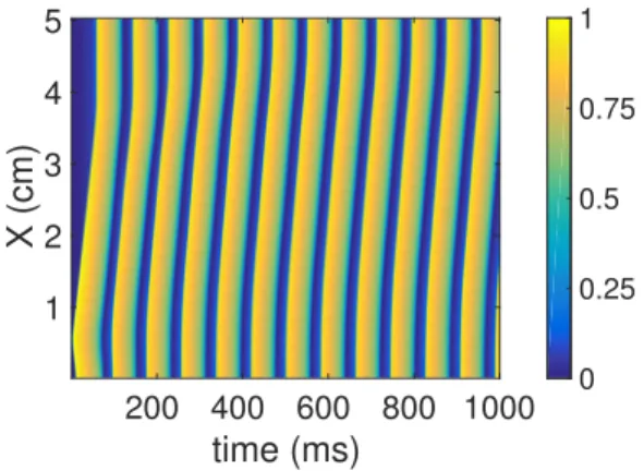
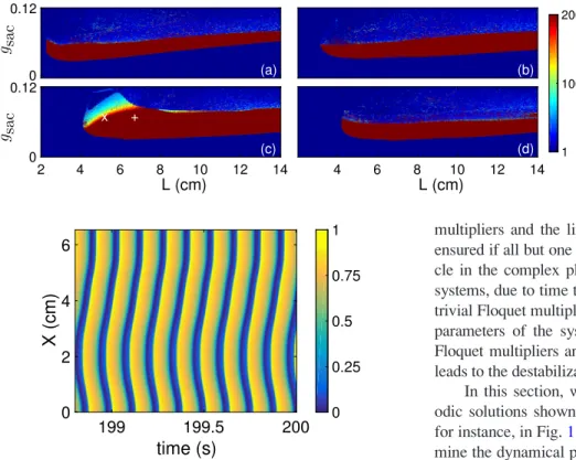
This behaviour is completely reversible in the simulated system (Figure 2). This parameter represents the extent of extracellular stimulation by an agonist. The

First introduced by Faddeev and Kashaev [7, 9], the quantum dilogarithm G b (x) and its variants S b (x) and g b (x) play a crucial role in the study of positive representations

A second scheme is associated with a decentered shock-capturing–type space discretization: the II scheme for the viscous linearized Euler–Poisson (LVEP) system (see section 3.3)..