Modeling, Simulation and Real-time Control of Active Filters

(1)

UNIVERSITÉ DE MONTRÉAL

MODELING, SIMULATION AND

REAL-TIME CONTROL OF ACTIVE FILTERS

ALIREZA JAVADI

DÉPARTEMENT DE GÉNIE ÉLECTRIQUE ÉCOLE POLYTECHNIQUE DE MONTRÉAL

MÉMOIRE PRÉSENTÉ EN VUE DE L’OBTENTION DU DIPLÔME DE MAÎTRISE ÈS SCIENCES APPLIQUÉES

(GÉNIE ÉLECTRIQUE) Decembre 2009

(2)

UNIVERSITÉ DE MONTRÉAL

ÉCOLE POLYTECHNIQUE DE MONTRÉAL

Ce mémoire intitulé:

MODELING, SIMULATION AND

REAL-TIME CONTROL OF ACTIVE FILTERS

Présenté par : JAVADI Alireza

En vue de l’obtention du diplôme de: Maîtrise ès sciences appliquées

a été dûment accepté par le jury d’examen constitué de : M. HURTEAU Richard, D.Ing., président

M. OLIVIER Guy M.

, Ph. D., membre et directeur de recherche SIROIS Frédéric

M.

, Ph. D., membre et codirecteur de recherche APRIL Georges-Émile, M. Sc., membre

(3)

DÉDICACE

To My Wife My Parents and All Family Members and Friends

(4)

ACKNOWLEDGMENT

I would like to say special thanks and offer special gratitude to my dear professor Guy Olivier for his excellent technical, moral support, and pedagogical guidance as my supervisor throughout the time that this research project has being carried out.

I would like to say special thanks to my dear co-supervisor, Mr. Frederic Sirois for his assistance and helpful advises during the laboratory tests.

I would like to also pay my gratitude and appreciations to my wife, my parents, and all family members and friends that have been of enormous help for the duration of this research work. My success in carrying out and completion of this project would certainly not have been possible without their generous supports.

(5)

RÉSUMÉ

Depuis toujours, la production et la distribution de l’énergie électrique à été réalisée en considérant que les ondes de tension et de courant étaient parfaitement sinusoïdales et que leur fréquence était fixe (50 ou 60 Hz). De fait, jusqu’au début des années quatre-vingt ces hypothèses étaient très largement vérifiées. Seuls quelques équipements produisaient des courants déformés non-sinusoïdaux : courants de magnétisation des transformateurs et de moteurs, ballasts de fluorescents et redresseurs ca/cc. Ces charges ne constituaient qu’une très faible partie des charges raccordées aux réseaux et n’avaient généralement aucune conséquence néfaste. Les progrès fantastiques de l’électronique ont complètement modifié la situation. Les téléviseurs couleur, les gradateurs pour l’éclairage, les équipements audio, les fours micro-onde et les ordinateurs personnels nécessitent tous l’emploi de convertisseurs électroniques pour fonctionner. En plus de ces appareils, l’industrie fait appel de plus en plus à des variateurs de vitesse pour les moteurs électriques eux aussi électroniques. Tous ces appareils constituent autant de sources de pollution harmonique. Même si, individuellement, leur puissance est faible, ensemble ils constituent une formidable source de pollution harmonique qui entraîne des conséquences sérieuses sur les réseaux électriques de basse et moyenne tension. En quelques années seulement, les problèmes associés à cette pollution harmonique sur la qualité de l’énergie électrique sont devenus l'un des problèmes les plus importants auxquels les ingénieurs doivent faire face.

Le rôle des filtres actifs est de compenser, sans consommé aucune puissance active, les harmoniques sur le système de transport d’énergie et d'améliorer l'efficacité du système électrique. La compensation de la puissance non-actif va considérablement augmenter le facteur de puissance et va réduire le coefficient de distorsion (THD) et aussi réduire les pertes. Cela signifie que le système peut laisser circuler plus de puissance active. Bien sûr, l'effet des harmoniques sur les appareils comme les transformateurs et les machines disparaîtra.

Le présent mémoire de maîtrise est consacré à la simulation et la commande en temps réel d'un filtre actif pour compenser et annuler les harmoniques de courant. On y propose tout d’abord un modèle de contrôle approprié pour le filtrage actif tiré de la littérature, pour ensuite simuler le modèle de contrôle du filtre à l’aide du logiciel Simulink de MATLAB et en faisant des

(6)

modification a l’aide du logiciel Opal-RT qui permet de réaliser l’interface avec le matériel physique, pour la commande en temps réel.

Finalement, le modèle sera implanté en laboratoire à l’aide des simulateurs en temps-réel de RT-Lab. sur le réseau triphasé de 120/240 V avec une charge non-linéaire constituée d’un redresseur triphasé. Les résultats expérimentaux obtenus en laboratoire démontrent une concordance avec les résultats obtenus par simulation. L’efficacité des différentes méthodes de commande et leur réponse transitoire font l’objet de comparaisons.

Enfin, ce mémoire propose trois recommandations pour la poursuite des travaux futurs dans ce domaine.

(7)

ABSTRACT

Historically, production and distribution of electricity were carried out taking into account that the voltage and current were perfectly sinusoidal and their frequency was fixed (50 or 60 Hz). In fact, prior to the early eighties, these assumptions were quite verified. Only few types of equipment generate deformed and non-sinusoidal currents: the magnetization current of transformers and motors, fluorescent ballasts and AC/ DC rectifiers. Actually, these equipments constituted a negligible portion of charges connected to the networks and generally did not introduce significant distortion. Fantastic progress in electronics has changed the situation. Color televisions, dimmers for lighting, audio equipments, microwave ovens and personal computers, all require the use of electronic converters to operate.

In addition to these devices, variable speed drives for industrial electric motors, which are made of electronic devices, are also other sources of harmonic pollution. Although, individually, their power is low, together they constitute a considerable source of harmonic pollutions which have serious consequences in the low or medium voltage power networks. In just a few years, issues of the harmonic pollution regarding the quality of electric power had become one of the most important problems that engineers should have confronted.

The role of active filters is to compensate harmonics in the power system and improve the efficiency of the electrical power system without any active power consumption. Compensation of non-active power substantially improves the power factor and reduces the total harmonic distortion index (THD) and also the total losses. This means that the system can transfer more active power with the same capacity. Another effect of harmonic compensation is the elimination of associated problems on electrical equipment such as transformers and electrical machines.

This master dissertation is dedicated to simulation and real-time control of an active filter to compensate current harmonics in a typical electric system. First, a control model appropriate for the active filter based on a literature review is proposed. Then, the control model is simulated using the Simulink toolbox of MATLAB. The model is then interfaced with the real world by using Opal-RT software to achieve an interconnection with the physical hardware for a real-time control. The final system constitutes a Hardware in the loop (HIL) application.

(8)

Finally, the model is implanted in laboratory with RT-Lab real-time Simulators to interact with a three phase 120/240 V system and a three phase rectifier as a non-linear load. Experimental results are also compared with simulation results. Moreover, the provided real-time structure makes it feasible to apply and compare different control designs and their transient state responses.

(9)

CONDENSÉ EN FRANÇAIS

0.1 Introduction

Les normes récentes imposent des limites sur les harmoniques qu’une installation peut injecter sur le réseau électrique qui l’alimente. Quelques solutions existent pour rencontrer ces exigences : filtres passifs, annulation magnétique sélective d’harmoniques au moyen de transformateurs déphaseurs, filtres actifs. Une autre approche est d’éviter à la source la génération d’harmoniques en concevant des redresseurs dits propres qui imposent une allure sinusoïdale aux courants qu’ils appellent du réseau. Ces solutions innovatrices, mais très chères ont été utilisées avec succès pour les ballasts de fluorescences et les blocs d’alimentation d’ordinateurs de dernière technologie. Malheureusement, ces technologies ne sont pas encore matures.

Une autre solution consiste à rendre les courants déformés sinusoïdaux en injectant un autre courant déformé de sorte que la somme des deux courants est une sinusoïde; ce sont les filtres actifs. Cette solution conceptuellement des plus attrayantes est complexe et très coûteuse à mettre en œuvre. La complexité de cette solution réside à la fois dans le calcul en temps réel du courant à injecter qui doit continuellement être recalculé en fonction du courant instantané de la charge à compenser et aussi dans la réalisation de l’onduleur qui doit littéralement fabriquer le courant compensatoire. La solution simultanée de ces deux problèmes exige des capacités très importantes de calcul en temps réel. Les premières solutions commerciales ont fait leur apparition. Mais beaucoup de travail reste à faire pour améliorer les performances et en réduire les coûts.

La compensation des harmoniques liez à la puissance non active est un moyen efficace pour résoudre le problème, résultant une amélioration dans la qualité de l'alimentation [34]. Les harmoniques de courant peuvent distraire la forme d’onde de la tension d'alimentation et produisent des résonances dans le réseau [5]. Il reste encore de nombreux problèmes, causés par les harmoniques, cruciales à régler. Le filtre actif est le principal enjeu technique pour faire face à ces problèmes [25]. De nombreuses approches ont été développées pour réaliser un compensateur variable instantané [1]. Cependant, leur efficacité n’a pas encore été testée dans la réalité afin d'assurer une compensation adéquate de la puissance non active.

(10)

0.2 Les définitions de puissance électrique

Il a été approuvé que les définitions classiques de la puissance électrique; active, réactive et apparente ne remplissent pas les conditions engendrées par les harmoniques et les déséquilibres. Par conséquent, des différentes définitions de puissance et des méthodes de calcul ont été proposées dans le domaine fréquentiel, ainsi que dans le domaine du temps. Trois définitions principales seront étudiées brièvement dans le deuxième chapitre pour donner une meilleure compréhension de la définition de puissance du réseau électrique dans les différentes conditions. La définition générale de puissance électrique définie par Budeanu, la définition de Depenbrock et Emanuel, ainsi que celle introduite par Czarnecki sera étudiée.

La définition couramment utilisée de la puissance établie par Budeanu peut être appliquée pour une analyse fréquentielle du système pour des situations sans distorsion. Cela signifie que pour une étude de puissance pour en cas de déséquilibré, les tensions et les courants peuvent être décomposée en série de Fourier pour calculer les harmoniques et les paramètres du système, comme le facteur de puissance. Il doit être prise en note que les méthodes utilisent dans le domaine fréquentiel ne peuvent être instantanée dans le temps, c'est pourquoi il convient de préciser que chaque méthode est applicable dans quel domaine.

Budeanu définit globalement quatre types de puissance pour un système monophasé; puissance apparente (S), puissance active (P), puissance réactive (Q), et la puissance de distorsion (D). Cette définition ne couvre pas tous les aspects des phénomènes tels que la distorsion et le déséquilibre, même le facteur de puissance dans certaines situations ne couvre pas toutes les parties de la puissance non active du système.

Depenbrock et Emanuel ont défini la puissance selon les concepts physiques de la puissance apparente, donc ces deux auteurs ont défini la puissance efficace (Se) étant la puissance active maximale transmissible pour une valeur rms déterminée de la tension et du courant. Cette définition a était développé après une étude plus complexe sur les définitions de Budeanu, afin de couvrir les contraints de l’ancienne approche. Leur définition est pratique et simple et peut être utilisée par les instruments de mesure. Chaque légère différence d'interprétation de la puissance conduit à une nouvelle définition.

(11)

Czarnecki a introduit un concept de décomposition orthogonale du courant pour la première fois en mars 1988. Czarnecki a proposé une définition plus attrayante dans laquelle le courant peut être décomposé en cinq composantes orthogonales qui contribuent à des phénomènes physiques différents. Mais il y a encore de l'incompétence dans cette définition.

0.3 La définition des puissances instantanées

Pour les systèmes monophasés, les notions telles que la puissance active et réactive, ainsi que le facteur de puissance sont bien définies. Diverses tentatives ont été proposées pour généraliser ces concepts à un système triphasé avec des courants et des tensions déséquilibrées et déformées. La plus récente théorie qui a était décrit par Akagi en 1984, introduit la notion de puissance réactive instantanée. Ce concept est très intéressant pour des raisons pratiques, en particulier pour analyser la compensation instantanée de la puissance réactive sans consommation d'énergie.

Après cette définition, des auteurs ont défini la théorie généralisée de la puissance, qui est une théorie plus complexe basée sur des calculs vectoriels applicables aux systèmes multiphasés. Par la suit Willems à proposer est un moyen simple et efficace pour réduire le processus de calcul. La théorie de Willems est basée sur la théorie du p-q et la décomposition orthogonale des courants.

Trois principales définitions de puissance instantanée sont présentées. La théorie de p-q instantanée d’Akagi est la première et principale théorie pour le calcul instantané des puissances sera présentée. Malheureusement, cette approche est limitée à un système triphasé. Bien que les calculs présentés par cette théorie sont simples, mais elles ne donnent pas un sens physique clair pour les différentes puissances. L'imprécision de cette méthode dépend de la probabilité d'obtenir une valeur infinie dans les différentes étapes de l'algorithme de contrôle. Les méthodes de contrôle dominant utilisé dans les filtres actifs industriels semblent être basées sur cette théorie en raison de sa rapidité.

La théorie généralisée de la puissance instantanée essaie d'étendre la théorie d’Akagi aux systèmes multiphasés. En utilisant les calculs vectoriels, il utilise l'idée d’Akagi, et donne une sensation plus physique aux concepts des puissances instantanées. En outre, de nombreux éléments indésirables apparaissent dans la compensation avec cette méthode qui fait en sorte que cette théorie soit moins pratique que la théorie de p-q instantanée.

(12)

Pour les systèmes de plus que trois phases, la théorie Willems pourrait être utile. Si l'objectif est d'obtenir un courant sinusoïdal de puissance ou de compenser toutes les puissances non actives, nous n’avons pas d'autre choix que la théorie généralisée. La théorie Willems est le meilleur choix si l'objectif est seulement de compenser la partie imaginaire (réactive) de la puissance instantanée. La méthode de Willem assure un facteur de puissance unitaire et compense la majorité des harmoniques présents dans le courant.

0.4 Résultats des essais de l’implantation du filtre actif en temps réel

Basé sur les théories étudiées et les simulations un contrôleur temps réel a été réalisé pour être mis en œuvre sur un simulateur en temps réel d’Opal-RT. Le contrôleur temps réel a été ensuite utilisé pour éliminer les harmoniques d'une charge non-linéaire. Les équipements utilisés en laboratoire pour ces essais seront présentés. Enfin, les résultats expérimentaux seront présentés et analysés.

En ce qui concerne la transformation de Clark sur un système en trois phases, la théorie p-q introduites par Akagi semble un bon départ pour réaliser un compensateur instantanée de la puissance réactive, mais dans le cas d’une compensation de la puissance non-active, d'autres méthodes devraient être utilisées. Bien entendu, l'hypothèse sera réfutée si les résultats des tests en temps réel montrent une compensation non instantanée ou une onde non-sinusoïdale du courant fourni par la source. La méthode proposée pour un test en temps réel est de simuler le filtre actif sur un simulateur d’Opal-RT pour le connecter à un système physique. Vue que la théorie d’Akagi pour la puissance instantanée (p-q instantanée) semble être le meilleure approche à nos jours. Donc, cette théorie a été utilisée pour la mise en œuvre dans le contrôleur en temps réel.

Enfin, le modèle a été mis en œuvre dans le laboratoire sur simulateur triphasé (120/240 V) et un redresseur triphasé entent que charge non-linéaire. Les résultats expérimentaux sont aussi comparés avec les résultats de simulation. Les instruments de test en temps réel, la procédure de l'essai, les résultats temps-réel seront présentés. Ce chapitre se concentre sur les tests et la méthodologie et la réalisation en temps réel d'un tel contrôleur.

Les équipements utilisés dans les tests vont être étudiées en détail. Le simulateur en temps-réel ainsi qu’un onduleur de puissance et une la charge non linéaire sont indispensables pour réaliser

(13)

ces tests. Certains instruments sont nécessaires pour réaliser un test en temps réel à cet effet la charge non linéaire qui est composée de deux redresseurs en parallèle et une charge résistive. Le simulateur en temps réel étant pas capable de produire des tensions et des courants suffisamment élevées, un onduleur de puissance a été utilisé pour produire le courant de compensation. Le simulateur en temps réel après avoir calculé le courant de compensation va générer les impulsions nécessaires qui vont être envoyé à l’onduleur pour produire le courant désiré.

Les résultats obtenus pour les différents essais sont figurées dans le quatrième chapitre de ce mémoire. Les résultats confirment que le projet a été réalisé avec succès. Par de tels résultats, il est possible de conclure que chaque partie du projet individuellement a été effectué correctement; la théorie du contrôle a était bien choisi, le modèle était un modèle approprié basé sur la théorie et le simulateur en temps réel a fonctionné correctement. Bien sûr, les autres éléments telle que l'onduleur et la charge non linéaire sont ajustés et ont fonctionné correctement pour ces essais.

L'objectif défini dans le projet était fondé sur un simple module de MLI (PWM) qui, en raison des résultats obtenus, l'auteur a été encouragé à aller plus loin pour développer un modulateur d'hystérésis (Hystérésis PWM). La modulation par hystérésis élimine les inconvénients du simple PWM. Même avec le block de PWM, le courant produit par l'onduleur a exactement la même forme que le courant de compensation. Un point faible dans cette méthode est que l'utilisation d'un filtre passif pour réduire l'amplitude des harmoniques autour de la fréquence de commutation est indispensable. L'autre point faible est l'absence d'un contrôle sur le courant produit par l’onduleur pendant le fonctionnement du filtre. Le deuxième problème disparait complètement en changeant le bloc PWM par un PWM avec hystérésis. La mise en œuvre du bloc PWM avec hystérésis a prolongé le projet avec une nécessité de faire une étude théorique, des simulations, la modélisation et l’intégration du bloc dans le contrôleur. Bien sûr de nombreuses configurations aurait dû être fait pour mettre la nouvelle méthode en marche.

L'utilisation du PWM avec hystérésis démontre la capacité de ces filtres. Ainsi grâce aux différents essais en temps réel, la capacité du filtre et la théorie utilisée pour les calculs a été illustré. Finalement, avec les essais durant un changement de charge, la réponse dynamique du filtre actif a été étudiée.

(14)

0.5 Conclusion

La production et la distribution d'énergie électrique ont été élaborées en considérant que la tension et le courant ont des formes d'onde parfaitement sinusoïdale. Avec les progrès de l'électronique, les questions de la qualité d’onde et la pollution causée par les harmoniques sont devenues l'un des problèmes les plus importants. Interférences de communication, les pertes par chauffage électrique, et les erreurs dans les coordinations des réseaux ont était les effets typiques indésirables des harmoniques.

Après une étude approfondie, quatre méthodes tirées de la littérature sont en mesure d'éliminer complètement ou partiellement le problème des distorsions dans les réseaux électriques; une inductance série dans la ligne, le filtre passif qui est une méthode relativement peu coûteuse, le transformateur Zigzag qui est appliqué pour les installations commerciales pour contrôler les composantes homopolaires des harmoniques, et finalement les filtres actifs qui sont relativement de nouveaux types de dispositifs destinés à éliminer les harmoniques. Ces types de filtres sont basés sur des appareils électroniques de puissance en les rendant plus fiables et plus flexibles que les autres méthodes mentionnées.

Dans ce mémoire de maîtrise un filtre actif a été modélisé et simulé pour assures un contrôle adéquat en temps réel des harmoniques de courant dans un système triphasé en laboratoire. L'objectif de ce projet a été accompli par une revue des théorèmes et les concepts de puissance électrique dans des conditions non sinusoïdales. Par la suite les algorithmes de contrôle ont été comparés. À cette fin, nous avons fait appel à la théorie de puissance instantanée d’Akagi (théorie p-q) qui est l'une des meilleures approches à nos jours. Finalement, un modèle de contrôle approprié pour le filtre actif basé sur les revues de littérature a été proposé. Le modèle de contrôle a été simulé pour assurer le bon fonctionnement du modèle.

Enfin, le modèle a été mis en œuvre en laboratoire sur un simulator en temps réel avec un redresseur triphasé comme charge non linéaire. Les résultats expérimentaux ont été comparés avec les résultats de simulation. En outre, grâce au circuit réalisé en laboratoire, il est possible de développer et de comparer les différentes conceptions de commande et leurs réponses en régime transitoire.

(15)

Les résultats expérimentaux illustrent un travail innovateur réalisé dans ce projet. Le modèle du filtre actif a pu compenser les harmoniques dans le réseau électrique et d'améliorer l'efficacité du système d'alimentation sans aucune consommation d'énergie active. La compensation de la non-puissance active améliore considérablement le facteur de puissance et réduit l'indice total de distorsion harmonique (THD), ainsi que les pertes totales dans le système. Cela signifie une évolution dans le domaine du réseau électrique, car le système aurait la capacité de transférer plus de puissance active avec la même capacité des installations. Les contributions de ce projet étaient: la réalisation d'un système en temps réel dans le laboratoire et la mise en œuvre en temps réel d’un filtre actif sur un système triphasé pour compenser les harmoniques d'une charge non linéaire.

En conclusion, les résultats obtenus en temps réel, démontrent que en utilisant les théories instantanées, il est possible de compenser les harmoniques et les autres problèmes de qualité d’énergie comme le du facteur de puissance pour un système triphasé avec ou sans le fil de neutre. Ces résultats démontrent que le simulateur en temps réel est en mesure de réaliser tout type de contrôleurs pour l’asservissement d’un réseau électrique en laboratoires.

(16)

LISTE OF TABLES

Table 3.1 Instantaneous reactive compensation ... 31 Table 3.2 Instantaneous powers ... 35 Table 4.1 Magnitude of each harmonic before and after compensation ... 86

(20)

LISTE OF FIGURES

Fig. 1.1 Low-pass broadband filter ... 3

Fig. 1.2 Power system with a shunt compensator on the load side ... 5

Fig. 2.1 Arithmetic SA, and Vector SV , apparent powers: Unbalanced nonsinusoidal conditions [6] ... 13

Fig. 3.1 Schema to better understand the physical meaning of the instantaneous powers ... 31

Fig. 3.2 Load voltage and current, source current, Instantaneous powers ... 32

Fig. 3.3 Instantaneous reactive compensation (𝑞𝑞) ... 33

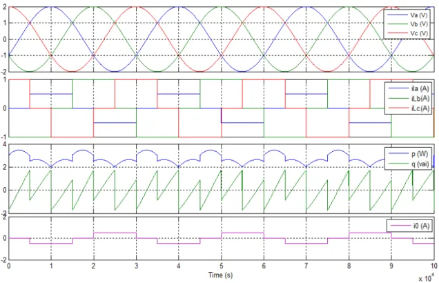
Fig. 3.4 Phase “a” voltage and current of load and source, source currents, instantaneous active and reactive power, load and source zero sequence current ( 𝑖𝑖0) ... 36

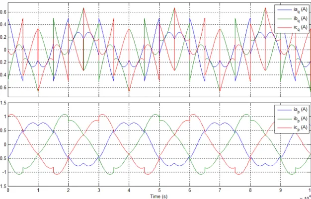
Fig. 3.5 a) load voltages and currents b) source currents c) instantaneous active and reactive power d) active filter zero-sequence current ( 𝑖𝑖0), e) compensation currents (𝑖𝑖𝑖𝑖𝑖𝑖, 𝑖𝑖𝑖𝑖𝑖𝑖)U ... 37

Fig. 3.6 Load, source, and active filter instantaneous active and reactive power ... 38

Fig. 3.7 Decomposition of current in a 3D space ... 41

Fig. 3.8 a) source voltages b) load currents c) instantaneous powers d) zero-sequence current of the load, for the case with zero phase degree ... 46

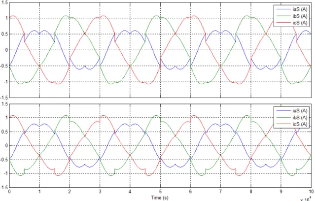
Fig. 3.9 Source currents a) without zero-sequence compensation b) with zero-sequence compensation for the case with zero phase degree ... 47

Fig. 3.10 Compensating current injected by the active filter, source currents for the case with zero phase degree ... 48

Fig. 3.11 a) Source voltages, b) load currents, c) instantaneous powers, d) zero-sequence current of the load for the case with 30 phase degree ... 49

Fig. 3.12 Source currents a) without zero-sequence compensation b) with zero-sequence compensation for the case with 30 phase degree ... 50

Fig. 3.13 Compensating current injected by the active filter, source currents for the case with 30 phase degree ... 51

(21)

Fig. 4.1 Power System laboratory at École Polytechnique de Montréal ... 54

Fig. 4.2 Two diode bridges connected in parallel ... 55

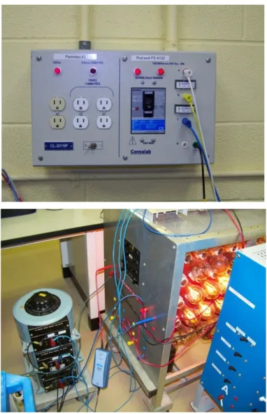
Fig. 4.3 The three phase source panel, the resistive load and the autotransformer ... 56

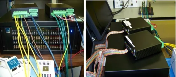
Fig. 4.4 The Probes and the patch panel, the probes and connection cables (front view) ... 57

Fig. 4.5 The real time simulator (MX-station), the analog card (left), the digital cards (right) .. ... 58

Fig. 4.6 The Probes and the patch panel, the probes and connections cables (front view) ... 58

Fig. 4.7 The three phase inverter, source for the electronic boards ... 59

Fig. 4.8 Schematic of the control of the active filter controller ... 61

Fig. 4.9 Under mask of the active filter controller block ... 62

Fig. 4.10 Hysteresis Block parameters ... 63

Fig. 4.11 Current-regulated voltage source inverter [36] ... 63

Fig. 4.12 Pulse width modulation (PWM) block, block parameters ... 64

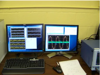
Fig. 4.13 Oscilloscopes view during the execution of the test ... 65

Fig. 4.14 Laboratory circuit block diagram ... 66

Fig. 4.15 Industrial active filter implementation block diagram with an energy storage component ... 67

Fig. 4.16 Instantaneous active, reactive and zero-sequence power of the non-linear load ... 69

Fig. 4.17 Instantaneous calculated compensating currents, carrier signal ... 70

Fig. 4.18 Instantaneous load, source, compensating and calculated currents ... 70

Fig. 4.19 The first phase (“a”) source voltage and current ... 71

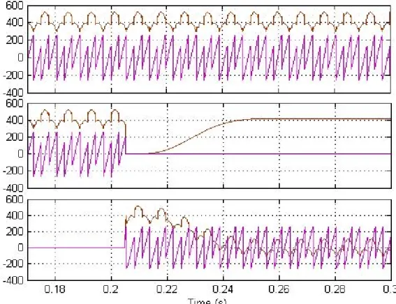
Fig. 4.20 The three phase voltages and currents, the dc voltage of the non-linear load ... 73

Fig. 4.21 Instantaneous active, reactive and zero-sequence powers, calculated compensation currents ... 73

(22)

Fig. 4.23 Instantaneous load, source, compensating and calculated currents for the second case ... 75 Fig. 4.24 The phase “a” source voltage and current for the second case ... 76 Fig. 4.25 The three phase voltages and currents, the dc voltage of the non-linear load ... 77 Fig. 4.26 Instantaneous active, reactive and zero-sequence powers, calculated compensation

currents for the third case ... 77 Fig. 4.27 Instantaneous load, source, compensating and calculated currents for the third case 78 Fig. 4.28 The first phase “a” source voltage and current for the third case ... 78 Fig. 4.29 The minimum margin calculation ... 80 Fig. 4.30 The three phase voltages and currents, the dc voltage of the non-linear load ... 81 Fig. 4.31 Instantaneous active, reactive and zero-sequence powers ... 81 Fig. 4.32 Instantaneous load, source, compensating and calculated currents for the case four 82 Fig. 4.33 The phase “a” source voltage and current for the case four ... 82 Fig. 4.34 Instantaneous load, source, compensating and calculated currents for the case five . 83 Fig. 4.35 The first phase “a” source voltage and current for the case five ... 84 Fig. 4.36 The frequency spectrum before and after harmonic compensation ... 85 Fig. 4.37 The fundamental, fifth, seventh, eleventh and thirteenth harmonic orders ... 85 Fig. 4.38 High order harmonics spectrum ... 86 Fig. 4.39 The three phase source voltages, the dc voltage of the non-linear load during

transient current tests ... 87 Fig. 4.40 The three phase load currents, the instantaneous active, reactive and zero-sequence

powers of the non-linear load for the decreasing load ... 88 Fig. 4.41 The calculated compensation currents, the phase “a” source voltage and current for

the decreasing load ... 88 Fig. 4.42 Instantaneous load, source, compensating and calculated currents during the change

(23)

Fig. 4.43 The three phase load currents ... 90 Fig. 4.44 The three phase load currents, the instantaneous active, reactive and zero-sequence

powers of the non-linear load for the increasing load ... 90 Fig. 4.45 The calculated compensation currents, the phase “a” source voltage and current for

the increasing load ... 91 Fig. 4.46 Instantaneous load, source, compensating and calculated currents during the increase

(24)

LISTE OF ABREVIATIONS

B Susceptance

C Capacitance

CSC Current source converter

D Distorted power

eff Effective value

f Frequency

FFT Fast Fourier transformation

G Conductance

h Harmonic order

H Henry

HIL Hardware in the loop

Hz Hertz

IGBT Insulated gate bipolar transistor

L Inductance N Non-active power ω Angular frequency P Active power PF Power factor PLL Phase-locked loop

PWM Pulse width modulation

Q Reactive power

(25)

rms Root mean square

s Second

S Apparent power

THD Total harmonic distortion

VA Volt-ampere

vai Volt-ampere imaginary var Volt-ampere reactive VSC Voltage source converter

W Watt

Z Impedance

M: 106 _{= 1 000 000} _mega

Multiple and sub-multiple of SI unities

k: 103 _{= 1 000} _kilo

m: 0.001 mili

µ: 10−6 _{= 0.000 001} _micro

𝑉𝑉�⃗ Vector in frequency domain Mathematical symbols

Bold (V or v) Matrix

Asterisk (V*) Complex conjugate

V rms value

v Instantaneous value

(26)

|𝑉𝑉| Absolute value

(27)

LISTE OF APPENDIX

APPENDIX I – Comparison for three phase- three wires system ... 99 APPENDIX II – Comparison for three phase- four wires system ... 100 APPENDIX III – Comparison of Generalized theory and Willems ... 102 APPENDIX IV – Published Papers ... 103

(28)

CHAPITRE 1 INTRODUCTION

1.1 Harmonic in Power Systems

In normal conditions, generated and distributed electric energy must be sinusoidal with predetermined frequency and magnitudes. Since the beginning of the power systems, there has been harmonic distortions due to nonlinear equipments such as generators, transformers, motors, etc. furthermore, harmonic pollution in power systems has significantly increased owing to large proliferation of power electronic devices. Consequently, the reactive power compensation in non-sinusoidal conditions became one of the most important problems in power systems.

Here some effects of harmonics on electric systems are counted:

• Communication interference; magnetic (or electrostatic) coupling between electrical power circuits and communication circuits can cause what is known as communication interference, induced line noise, interference with power line carrier systems and relay malfunctions.

•_{Losses as heating; it is common to refer to heating as 𝑅𝑅. 𝐼𝐼}2_{losses. By using}

superposition, the total losses can be expressed as sum of individual harmonic losses, excessive losses and overheating of transformers, motors, capacitors, and blown capacitor fuses.

• Solid-state device malfunctions; harmonics can cause solid-state devices to malfunction if the equipment is sensitive to zero crossings. A resonance condition can cause a current waveform to have zero crossings occur more than once every half-cycle, nuisance tripping of relays and breakers, errors in measurement equipment, unstable operation of zero voltage crossing firing circuits and interference with motor controllers.

• Neutral currents; which flow into the system and causes additional losses and other associated problems.

(29)

1.2 Harmonic Current and Voltage Sources

The Power quality problems caused by single phase rectifier loads are well known. Electronic equipments used for data processing such as laptops, typically features a simple diode bridge rectifier at the front end of the power circuit. The rectifier, in conjunction with its capacitive filter is a nonlinear load and draws current with high crest factor and rich in harmonics, resulting in power quality problems. They also contribute adversely by degrading the supply voltage waveform. Moreover they cause overheating of transformers and neutral conductors, create equipment malfunction and inefficient use of electric energy.

With the modern technology, it is possible to rectify the three phase ac power to dc power using static rectifiers for dc drives as well as static inversion for ac drives. Though more versatile than past methods, these newer technologies may have detrimental effects on the quality of the ac system, especially when they comprise a significant portion of the system. Rectification generates harmonic voltages and currents that can cause problems; middle of the harmonic distortion range can lead to insulation failures due to overheating and over voltages, malfunction of solid-state equipments, communication interference, overheating of motors, transformers and generators and also can excite system resonances, etc. The common addition of power factor correction capacitors to such a system generally increases the likelihood occurrence of such problems. Lower frequencies such as inter-harmonics may cause torque problems for shafts of motors and generators.

All the devices with nonlinear characteristics that derive their input power from a sinusoidal electrical system may be responsible for injecting harmonic currents and voltages into the electrical system. The principal sources of undesirable harmonics are rectifiers and electric arc furnaces. The common applications of rectifiers are solid-state drives and uninterruptible power supplies (UPS). Nowadays with the increment of nonlinear loads in the electric grids, these problems are not only isolated but much more common than in the past.

1.3 Harmonic Compensation Methods

A simple mitigation action such as adding a shunt capacitor bank can effectively modify an unfavorable system frequency response, and so reduce the harmonics to an acceptable level.

(30)

i. In-line reactor

In-line reactor or choke is a simple solution to control harmonic distortion generated by adjustable speed drives. The solution is come up with inserting a relatively small reactor, or choke, at the input of the drive. The inductance prevents the capacitor to be charged in a short time and forces the drive to draw current over a longer time and reduces the magnitude of the current with much less harmonic content while still delivering the same energy.

ii. Passive filters

Passive filter, which is relatively inexpensive in comparison with the other harmonic reduction methods, is the most used method. Inductance, capacitor and the load as a resistance are tuned in a way to control the harmonics. However, they suffer from interfering with the power systems. Actually, passive filters are designed to shunt harmonics from the lines or block their flow through some parts of the systems by tuning the elements to create a resonance at the selected frequency.

These filters are tuned and fixed according to the impedance of the point at which they will be connected and hence cannot be adjusted instantaneously in accordance to the load. As a result their cutoff frequency changes unexpectedly after any change in the load impedance resulting in producing a resonance with other elements installed in the system. The most common type of shunt passive filter is the single tuned (notch) filter which is a combination of an inductance and a capacitor. The other one is the low-pass broadband filter which is an inductor in series and a capacitor bank in parallel with the power system as shown in the figure 1.1.

Fig. 1.1 Low-pass broadband filter + L

+

(31)

iii. Zigzag transformers

Zigzag transformers are applied for commercial facilities to control zero-sequence harmonic components. The Zigzag transformers are not being used only as ordinary transformers; they additionally act as filters for zero-sequence currents by offering low impedance paths to neutral. This reduces the amount of current that flows in the neutral back toward the supply by providing a shorter path for the current.

iv. Active filters

Active filters are relatively new types of devices for eliminating harmonics. This kind of filter is based on power electronic devices and is much more expensive than passive filters. They have the distinct advantage that they do not resonate with the power system and they work independently with respect to the system impedance characteristics. They are used in difficult circumstances where passive filters don’t operate successfully because of resonance problems and they don’t have any interference with other elements installed anywhere in the power system. They can also address more than one harmonic at the same time and solve other power quality problems like flicker, etc.

They are particularly useful for large distorting loads fed from relatively weak points on the system. The most important advantage of theses filters is their ability to be adjusted instantly with the load changes without any energy storage components, so they can compensate harmonics completely without consuming any active power and there is no need to be frequently adapted to the load changes. In addition, they can provide compensating current from zero to their maximum capacity according to the load currents; so if the load does not need any compensating current, the compensators will not inject any current and even if the frequency of harmonics of the load changes, the filters can easily adapt to compensate the new harmonics without any need for tuning in the hardware.

Active filters inject a current to the junction point in a way that the sum of the compensating and the load current become a sinusoidal wave form seen from the source as illustrated in figure 1.2. The substantial issue of active filters is how to calculate the suitable compensating current which will be clarified in the next chapter. Active filters are also being programmed to do power factor correction as well as harmonic suppression.

(32)

Fig. 1.2 Power system with a shunt compensator on the load side

1.4 Master dissertation Objectives

The first objective of this project is to go over the theorems and definitions of electric power concepts under non-sinusoidal conditions. In this manner we will see the harmonics causes and effects such as their flow in the power system and their contribution on the decrease of power indexes. In the second part we will survey different interpretation of active and reactive power and their ability to be used in the control algorithm of active filters. Then we will recall Akagi’s theory of instantaneous power (p-q theory) and limitations of this approach. Moreover, we will make a study on the real-time harmonic and reactive compensation principles. Furthermore a brief study on active filters and their ability to actively clean the network from harmonics, to smooth reactive power and making a load balancing, will be done. Then a real-time modeling of an active filter in the MATLAB Simulink environment using Opal-RT block sets should be done. The last objective is to make Real-time implementation and control of an active filter using RT-lab simulator which dedicates the final part of the dissertation.

(33)

1.5 Methodology

At first we have review the concepts of electrical power definitions and their traditional approaches. The mechanism of harmonic generation and its effects on unbalanced systems is then studied. Consequently, the study of the instantaneous active and reactive power and the p-q theory of Akagi follow.

Different definitions of non-active power and compensable power theories found in the literatures are also compared. Moreover active filters and their compensation approaches are surveyed.

We will simulate the control block of an active filter in the Simulink environment to compensate the non-active power in balanced and unbalanced distorted conditions. In order to make the interfaces between physical instruments and the model in Simulink, the model will be modified with Opal-RT block sets. Then the model will be implemented in the real-time simulator to make the active filter controlled in real-time mode.

(34)

CHAPITRE 2 ELECTRIC POWER DEFINITIONS

2.1 Introduction

It has been generally accepted that classical definitions of electric power (active, reactive and apparent power) does not fulfill the conditions resulting from the existence of by harmonics and unbalances conditions. Consequently, various power definitions and calculation methods have been proposed in frequency domain and even in time domain to cover as much as the matter. Three main proposed definitions will be studied briefly in this chapter to give a better understanding of electrical powers definition in different situations. General power definition based on Budeanu, Depenbrock and Emanuel definitions will be presented, and finally the Czarnecki contribution on electrical powers will be studied.

In the same way many theories have been developed to control the active filters to achieve compensation of the unwanted harmonics from the network. The time domain approach due to Akagi Nabae under the name of “p-q theory” or “instantaneous power theory” is the most dominant theory for two or three phases and three or four wire but this method has some conceptual limitations which many contributors have attempted to resolve these limitations and associated problems that will be explained and clarified in the next chapter.

2.2 General powers definition

The commonly used definition of power established by Budeanu for a frequency domain analysis can be applied for a steady state analysis. That means for a steady state study voltages and currents could be decomposed in Fourier series to calculate harmonics and each parameter of the system like powers and power factors. It should be noticed that since the method use frequency domain it cannot be instantaneous in the time domain; therefore it should be clarified that each method is used for which domain of study.

2.2.1 Budeanu’s definition

Budeanu globally defines four types of power for a single phase case; apparent power (S), active power (P), reactive power (Q), and distorted power (D).

(35)

For single phase, the following powers can be derived from Budeanu’s definitions: Apparent power S: 𝑆𝑆 = 𝑉𝑉𝐼𝐼 = ��∞ 𝑉𝑉_𝑘𝑘2 𝑘𝑘=1 × �� 𝐼𝐼𝑘𝑘 2 ∞ 𝑘𝑘=1 (2-1) Active power P: 𝑃𝑃 = � 𝑃𝑃𝑘𝑘 ∞ 𝑘𝑘=1 = � 𝑉𝑉𝑘𝑘𝐼𝐼𝑘𝑘𝑐𝑐𝑐𝑐𝑐𝑐 𝜑𝜑𝑘𝑘 ∞ 𝑘𝑘=1 (2-2) Reactive power Q: 𝑄𝑄 = � 𝑄𝑄𝑘𝑘 ∞ 𝑘𝑘=1 = � 𝑉𝑉𝑘𝑘𝐼𝐼𝑘𝑘𝑐𝑐𝑖𝑖𝑠𝑠 𝜑𝜑𝑘𝑘 ∞ 𝑘𝑘=1 (2-3) Distortion power D: 𝐷𝐷 = �𝑆𝑆2_{− 𝑃𝑃}2_{− 𝑄𝑄}2 (2-4)

(36)

2.2.2 Instantaneous power (W)

This definition in time-domain is common for all definitions with the unit of watt (W). It should be noticed that this power differs from the general active power in frequency domain which is an average of the instantaneous power in a cycle.

In three phase systems, with 3 or 4 wires the instantaneous voltages and currents are shown as an instantaneous space vector v and i.

𝒗𝒗 = �𝑣𝑣𝑣𝑣𝑎𝑎𝑠𝑠𝑏𝑏𝑠𝑠

𝑣𝑣𝑐𝑐𝑠𝑠

� , 𝒊𝒊 = �𝑖𝑖𝑖𝑖𝑎𝑎𝑏𝑏

𝑖𝑖𝑐𝑐

� (2-5)

𝑣𝑣𝑘𝑘𝑠𝑠 - Phase to ground voltage.

𝑖𝑖𝑘𝑘 - Phase current.

The instantaneous active power is defined as:

𝑝𝑝 = 𝑣𝑣⃗∙ 𝑖𝑖⃗ = 𝑣𝑣𝑎𝑎𝑠𝑠𝑖𝑖𝑎𝑎 + 𝑣𝑣𝑏𝑏𝑠𝑠𝑖𝑖𝑏𝑏 + 𝑣𝑣𝑐𝑐𝑠𝑠𝑖𝑖𝑐𝑐 (2-6)

For balanced three wire systems where ia + ib + ic = 0, and it is possible to take one of the

voltages as reference, and obtain the following relations:

𝑝𝑝 = (𝑣𝑣𝑎𝑎 − 𝑣𝑣𝑏𝑏)𝑖𝑖𝑎𝑎 + (𝑣𝑣𝑏𝑏 − 𝑣𝑣𝑏𝑏)𝑖𝑖𝑏𝑏 + (𝑣𝑣𝑐𝑐 − 𝑣𝑣𝑏𝑏)𝑖𝑖𝑐𝑐 (2-7)

𝑝𝑝 = 𝑣𝑣𝑎𝑎𝑏𝑏𝑖𝑖𝑎𝑎 + 𝑣𝑣𝑐𝑐𝑏𝑏𝑖𝑖𝑐𝑐 = 𝑣𝑣𝑎𝑎𝑐𝑐𝑖𝑖𝑎𝑎 + 𝑣𝑣𝑏𝑏𝑐𝑐𝑖𝑖𝑏𝑏 = 𝑣𝑣𝑏𝑏𝑎𝑎𝑖𝑖𝑏𝑏 + 𝑣𝑣𝑐𝑐𝑎𝑎𝑖𝑖𝑐𝑐 (2-8)

(37)

2.2.3 Active power (W)

Active power is the mean of the instantaneous power in the time period.

𝑃𝑃 =_{𝑘𝑘𝑘𝑘 �}1 𝑣𝑣𝑖𝑖𝑖𝑖𝑖𝑖𝑑𝑑𝑑𝑑 𝜏𝜏+𝑘𝑘𝑘𝑘

𝜏𝜏 𝑖𝑖 = 𝑎𝑎, 𝑏𝑏, 𝑐𝑐

(2-9)

The line-to-neutral voltages are as follows:

𝑣𝑣𝑖𝑖 = √2 � 𝑉𝑉𝑖𝑖ℎ 𝑠𝑠 ℎ=1

𝑐𝑐𝑖𝑖𝑠𝑠(ℎ𝜔𝜔𝑑𝑑 + 𝑖𝑖ℎ ± 120𝑐𝑐ℎ) 𝑖𝑖 = 𝑎𝑎, 𝑏𝑏, 𝑐𝑐

(2-10)

The line currents have similar expressions:

𝑖𝑖𝑖𝑖 = √2 � 𝐼𝐼𝑖𝑖ℎ 𝑠𝑠 ℎ=1

𝑐𝑐𝑖𝑖𝑠𝑠(ℎ𝜔𝜔𝑑𝑑 + 𝑖𝑖ℎ ± 120𝑐𝑐ℎ) 𝑖𝑖 = 𝑎𝑎, 𝑏𝑏, 𝑐𝑐

(2-11)

V and I are rms values.

For a general case in the frequency domain, using the Fourier series and sequence transformation, voltages and currents are decomposed in their rms values, and the active power is defined as follows:

𝑃𝑃 = � 𝑉𝑉𝑘𝑘𝐼𝐼𝑘𝑘cos(𝜃𝜃𝑘𝑘) =

= 𝑉𝑉1𝑑𝑑𝐼𝐼1𝑑𝑑cos(𝜃𝜃1𝑑𝑑) + 𝑉𝑉2𝑑𝑑𝐼𝐼2𝑑𝑑cos(𝜃𝜃2𝑑𝑑) + 𝑉𝑉3𝑑𝑑𝐼𝐼3𝑑𝑑cos(𝜃𝜃3𝑑𝑑) + ⋯

+𝑉𝑉1𝑖𝑖𝐼𝐼1𝑖𝑖cos(𝜃𝜃1𝑖𝑖) + 𝑉𝑉2𝑖𝑖𝐼𝐼2𝑖𝑖cos(𝜃𝜃2𝑖𝑖) + ⋯

+𝑉𝑉1𝑂𝑂𝐼𝐼1𝑂𝑂cos(𝜃𝜃1𝑂𝑂) + 𝑉𝑉2𝑂𝑂𝐼𝐼2𝑂𝑂cos(𝜃𝜃2𝑂𝑂) + ⋯

(2-12)

(38)

2.2.4 Reactive power (var)

The reactive power is defined as follows:

𝑄𝑄 = � 𝑉𝑉𝑘𝑘𝐼𝐼𝑘𝑘𝑐𝑐𝑖𝑖𝑠𝑠(𝜃𝜃𝑘𝑘) =

= 𝑉𝑉1𝑑𝑑𝐼𝐼1𝑑𝑑𝑐𝑐𝑖𝑖𝑠𝑠(𝜃𝜃1𝑑𝑑) + 𝑉𝑉2𝑑𝑑𝐼𝐼2𝑑𝑑𝑐𝑐𝑖𝑖𝑠𝑠(𝜃𝜃2𝑑𝑑) + 𝑉𝑉3𝑑𝑑𝐼𝐼3𝑑𝑑𝑐𝑐𝑖𝑖𝑠𝑠(𝜃𝜃3𝑑𝑑) + ⋯

+𝑉𝑉1𝑖𝑖𝐼𝐼1𝑖𝑖𝑐𝑐𝑖𝑖𝑠𝑠(𝜃𝜃1𝑖𝑖) + 𝑉𝑉2𝑖𝑖𝐼𝐼2𝑖𝑖𝑐𝑐𝑖𝑖𝑠𝑠(𝜃𝜃2𝑖𝑖) + ⋯

+𝑉𝑉1𝑂𝑂𝐼𝐼1𝑂𝑂𝑐𝑐𝑖𝑖𝑠𝑠(𝜃𝜃1𝑂𝑂) + 𝑉𝑉2𝑂𝑂𝐼𝐼2𝑂𝑂𝑐𝑐𝑖𝑖𝑠𝑠(𝜃𝜃2𝑂𝑂) + ⋯

(2-13)

2.2.5 Apparent power (VA)

It is possible to define two different apparent powers;

2.2.5.1 Arithmetic apparent power SA

This definition is an extension of Budeanu’s apparent power resolution for single-phase systems. SA the sum of magnitude of apparent power for each phase:

𝑆𝑆𝑎𝑎 = �𝑃𝑃𝑎𝑎2+ 𝑄𝑄𝑎𝑎2+ 𝐷𝐷𝑎𝑎2 (2-14)

𝑆𝑆𝑏𝑏 = �𝑃𝑃𝑏𝑏2+ 𝑄𝑄𝑏𝑏2 + 𝐷𝐷𝑏𝑏2 (2-15)

𝑆𝑆𝑐𝑐 = �𝑃𝑃𝑐𝑐2+ 𝑄𝑄𝑐𝑐2+ 𝐷𝐷𝑐𝑐2 (2-16)

The following arithmetic apparent power is obtained:

𝑆𝑆𝐴𝐴 = 𝑆𝑆𝑎𝑎 + 𝑆𝑆𝑏𝑏+ 𝑆𝑆𝑐𝑐 (2-17)

The power factor is obtained: 𝑃𝑃𝑃𝑃𝐴𝐴 = 𝑃𝑃 𝑆𝑆� _𝐴𝐴 (2-18)

Di is the Budeanu’s Distortion power (var).

(39)

2.2.5.2 Vector apparent power SV

SV is the vector sum of phase apparent power:

𝑆𝑆𝑉𝑉 �� =_𝑆𝑆 𝑎𝑎 → +_𝑆𝑆 𝑏𝑏 → +_𝑆𝑆 𝑐𝑐 → (2-20) |𝑆𝑆𝑉𝑉| = �𝑃𝑃2+ 𝑄𝑄2 + 𝐷𝐷2 (2-21) Where 𝑃𝑃 = 𝑃𝑃𝑎𝑎 + 𝑃𝑃𝑏𝑏 + 𝑃𝑃𝑐𝑐 (2-22) 𝑄𝑄 = 𝑄𝑄𝑎𝑎 + 𝑄𝑄𝑏𝑏 + 𝑄𝑄𝑐𝑐 (2-23) 𝐷𝐷 = 𝐷𝐷𝑎𝑎 + 𝐷𝐷𝑏𝑏 + 𝐷𝐷𝑐𝑐 (2-24)

It is possible to separate the active and reactive power from distortion part:

𝑆𝑆′ = 𝑃𝑃 + 𝑄𝑄 (2-25) |𝑆𝑆′| = �𝑃𝑃2_{+ 𝑄𝑄}2 ₌ (2-26) �|𝑉𝑉𝑘𝑘|. |𝐼𝐼𝑘𝑘| = �( |𝑉𝑉ℎ𝑑𝑑||𝐼𝐼ℎ𝑑𝑑| + |𝑉𝑉ℎ𝑖𝑖||𝐼𝐼ℎ𝑖𝑖| + |𝑉𝑉ℎ𝑂𝑂||𝐼𝐼ℎ𝑂𝑂| ) ∞ ℎ=1 (2-27)

Budeanu’s reactive power Q can be completely compensated with a simple capacitor; however this is not the case for the distortion power D. It is possible to demonstrate that P, Q, and D are two by two orthogonal, which is illustrated in figure 2.1.

(40)

Fig. 2.1 Arithmetic SA, and Vector SV , apparent powers: Unbalanced nonsinusoidal conditions [6]

2.2.6 Author’s contribution

If we suppose that: |𝑆𝑆| = |𝑉𝑉|. |𝐼𝐼| (2-29) Where |𝑉𝑉| = ∑ �|𝑉𝑉ℎ ℎ𝑑𝑑|2+ |𝑉𝑉ℎ𝑖𝑖|2+ |𝑉𝑉ℎ𝑂𝑂|2 (2-30) |𝐼𝐼| = � �|𝐼𝐼ℎ𝑑𝑑|2+ |𝐼𝐼ℎ𝑖𝑖|2+ |𝐼𝐼ℎ𝑂𝑂|2 ℎ (2-31)

(41)

It is possible to divide the apparent power into three main powers: 𝑆𝑆2 _{= 𝑆𝑆′}2_{+ 𝐷𝐷}2 _{+ 𝑈𝑈}2 _{= �|𝑉𝑉} 1𝑑𝑑|2× �|𝐼𝐼1𝑑𝑑|2 + |𝐼𝐼1𝑖𝑖|2+ |𝐼𝐼1𝑂𝑂|2 + |𝐼𝐼2𝑑𝑑|2+ |𝐼𝐼2𝑖𝑖|2+ ⋯ (2-33) |𝑆𝑆′| = �𝑃𝑃2_{+ 𝑄𝑄}2 _{= �|𝑉𝑉|}2_|𝐼𝐼_1𝑑𝑑_|2 (2-34) 𝐷𝐷 = �|𝑉𝑉|2_|𝐼𝐼_ℎ𝑑𝑑_|2 (2-35) 𝑈𝑈 = �|𝑉𝑉|2_|𝐼𝐼_𝑖𝑖_|2 _{+ |𝑉𝑉|}2_|𝐼𝐼_𝑂𝑂_|2 (2-36) �_|𝐼𝐼|𝐼𝐼𝑖𝑖|2 = |𝐼𝐼1𝑖𝑖|2+ |𝐼𝐼ℎ𝑖𝑖|2 𝑂𝑂|2 = |𝐼𝐼1𝑂𝑂|2+ |𝐼𝐼ℎ𝑂𝑂|2 (2-37)

Where suffix h is the number of harmonics, D is the distortion power, U is the power associated with the unbalances and is named the unbalance power, and S’ is the fundamental apparent power. All these powers are two by two orthogonal; 𝐷𝐷 ⊥ 𝑆𝑆′_{, 𝑈𝑈 ⊥ 𝑆𝑆}′_{, 𝐷𝐷 ⊥ 𝑈𝑈.}

(42)

2.3 Depenbrock and Emanuel definition

According to physical concepts of apparent power these two authors define the effective power (Se) as the maximum transmittable active power for a given rms value of the voltage and

the given rms value of the current. This equivalence leads to the definition of an effective line current Ieff and an effective line-to-neutral voltage Veff .

𝑉𝑉𝑒𝑒𝑒𝑒𝑒𝑒 = �𝑉𝑉𝑒𝑒𝑒𝑒𝑒𝑒 12 + 𝑉𝑉𝑒𝑒𝑒𝑒𝑒𝑒 ℎ2 , 𝐼𝐼𝑒𝑒𝑒𝑒𝑒𝑒 = �𝐼𝐼𝑒𝑒𝑒𝑒𝑒𝑒 12 + 𝐼𝐼𝑒𝑒𝑒𝑒𝑒𝑒 ℎ2 (2-38)

Where for a four-wire system:

𝐼𝐼𝑒𝑒𝑒𝑒𝑒𝑒 = �𝐼𝐼𝑎𝑎 2_{+ 𝐼𝐼} 𝑏𝑏2+ 𝐼𝐼𝑐𝑐2+ 𝐼𝐼𝑠𝑠2 3 (2-39) 𝑉𝑉𝑒𝑒𝑒𝑒𝑒𝑒 = �1 18� [𝑉𝑉𝑎𝑎𝑏𝑏2 + 𝑉𝑉𝑏𝑏𝑐𝑐2 + 𝑉𝑉𝑐𝑐𝑎𝑎2 + 3(𝑉𝑉𝑎𝑎2+ 𝑉𝑉𝑏𝑏2 + 𝑉𝑉𝑐𝑐2)] (2-40)

The In denotes the neutral current.

The apparent power is defined consequently:

𝑆𝑆𝑒𝑒𝑒𝑒𝑒𝑒 = 𝑉𝑉𝑒𝑒𝑒𝑒𝑒𝑒. 𝐼𝐼𝑒𝑒𝑒𝑒𝑒𝑒 (2-41)

They divide the apparent power into two main partitions, the active power (P) and the non-active power (N).

𝑃𝑃(𝑊𝑊) = 𝑃𝑃1+ 𝑃𝑃ℎ (2-42)

𝑁𝑁(𝑣𝑣𝑎𝑎𝑣𝑣 )= �𝑆𝑆𝑒𝑒𝑒𝑒𝑒𝑒2 − 𝑃𝑃2 (2-43)

The indice h defines the harmonic number.

(43)

𝑃𝑃ℎ = � 𝑉𝑉𝑖𝑖ℎ𝐼𝐼𝑖𝑖ℎcos(𝜃𝜃𝑖𝑖ℎ) 𝑖𝑖 = 𝑎𝑎, 𝑏𝑏, 𝑐𝑐 ∞ ℎ≠1 (2-45) 𝑆𝑆 1𝑑𝑑 = 𝑃𝑃1𝑑𝑑 + 𝑗𝑗𝑄𝑄1𝑑𝑑 = 3𝑉𝑉𝑒𝑒𝑒𝑒𝑒𝑒 1𝑑𝑑𝐼𝐼𝑒𝑒𝑒𝑒𝑒𝑒 1𝑑𝑑 (2-46) 𝑆𝑆𝑒𝑒𝑒𝑒𝑒𝑒 12 = 𝑆𝑆1𝑑𝑑2 + 𝑆𝑆𝑈𝑈12 (2-47)

The Seff 1 is the fundamental effective apparent power. The reactive power (Q1d) is the

conventional power to determine the amount of capacitor bank needed to compensate the conventional power factor.

The fundamental positive-sequence power factor (PF1) is obtained from the following

equation and plays the same significant role that the fundamental power factor does in non-sinusoidal single phase systems.

𝑃𝑃𝑃𝑃1 = 𝑃𝑃_𝑆𝑆1𝑑𝑑 1𝑑𝑑

(2-48)

The load unbalance is evaluated by the fundamental unbalanced power (SU1) from the

following equation.

𝑆𝑆𝑈𝑈 12 = �(3𝑉𝑉𝑒𝑒𝑒𝑒𝑒𝑒 1𝐼𝐼𝑒𝑒𝑒𝑒𝑒𝑒 1)2− (3𝑉𝑉𝑒𝑒𝑒𝑒𝑒𝑒 1𝑑𝑑𝐼𝐼𝑒𝑒𝑒𝑒𝑒𝑒 1𝑑𝑑)2 (2-49)

The apparent power is divided into the fundamental effective apparent power (Seff 1) and the

non-fundamental effective apparent power (Seff N).

𝑆𝑆𝑒𝑒𝑒𝑒𝑒𝑒2 = 𝑆𝑆𝑒𝑒𝑒𝑒𝑒𝑒 12 + 𝑆𝑆𝑒𝑒𝑒𝑒𝑒𝑒 𝑁𝑁2 (2-50)

𝑆𝑆𝑒𝑒𝑒𝑒𝑒𝑒 𝑁𝑁 = 3�(𝑉𝑉𝑒𝑒𝑒𝑒𝑒𝑒 ℎ𝐼𝐼𝑒𝑒𝑒𝑒𝑒𝑒 ℎ)2+ (𝑉𝑉𝑒𝑒𝑒𝑒𝑒𝑒 ℎ𝐼𝐼𝑒𝑒𝑒𝑒𝑒𝑒 1)2+ (𝑉𝑉𝑒𝑒𝑒𝑒𝑒𝑒 1𝐼𝐼𝑒𝑒𝑒𝑒𝑒𝑒 ℎ)2 (2-51)

The non-fundamental effective apparent power (Seff N) is resolved into three distinctive terms:

(44)

the voltage distortion power (var) 𝐷𝐷𝑒𝑒𝑒𝑒𝑒𝑒 𝑉𝑉 = 3. 𝑉𝑉𝑒𝑒𝑒𝑒𝑒𝑒 ℎ. 𝐼𝐼𝑒𝑒𝑒𝑒𝑒𝑒 1 (2-53)

the current distortion power (var) 𝐷𝐷𝑒𝑒𝑒𝑒𝑒𝑒 𝐼𝐼 = 3. 𝑉𝑉𝑒𝑒𝑒𝑒𝑒𝑒 1. 𝐼𝐼𝑒𝑒𝑒𝑒𝑒𝑒 ℎ (2-54)

and the harmonic apparent power itself is divided into active and reactive parts:

𝑆𝑆𝑒𝑒𝑒𝑒𝑒𝑒 ℎ = 𝑃𝑃ℎ + 𝑗𝑗𝑄𝑄ℎ (2-55)

By defining the equivalent total harmonic distortions as follow:

𝑘𝑘𝑇𝑇𝐷𝐷𝑒𝑒𝑒𝑒𝑒𝑒 𝑉𝑉 = 𝑉𝑉𝑒𝑒𝑒𝑒𝑒𝑒 ℎ�_𝑉𝑉_{𝑒𝑒𝑒𝑒𝑒𝑒 1} , 𝑘𝑘𝑇𝑇𝐷𝐷𝑒𝑒𝑒𝑒𝑒𝑒 𝐼𝐼 = 𝐼𝐼𝑒𝑒𝑒𝑒𝑒𝑒 ℎ�_𝐼𝐼_{𝑒𝑒𝑒𝑒𝑒𝑒 1} (2-56)

The non-fundamental effective apparent power is also obtained from:

𝑆𝑆𝑒𝑒𝑒𝑒𝑒𝑒 𝑁𝑁 = 𝑆𝑆𝑒𝑒𝑒𝑒𝑒𝑒 1�(𝑘𝑘𝑇𝑇𝐷𝐷𝑒𝑒𝑒𝑒𝑒𝑒 𝑉𝑉𝑘𝑘𝑇𝑇𝐷𝐷𝑒𝑒𝑒𝑒𝑒𝑒 𝐼𝐼)2 + 𝑘𝑘𝑇𝑇𝐷𝐷𝑒𝑒𝑒𝑒𝑒𝑒 𝑉𝑉2+ 𝑘𝑘𝑇𝑇𝐷𝐷𝑒𝑒𝑒𝑒𝑒𝑒 𝐼𝐼2 (2-57)

So the general power factor under this approach is:

𝑃𝑃𝑃𝑃 =_𝑆𝑆𝑃𝑃

𝑒𝑒𝑒𝑒𝑒𝑒

(45)

2.4 Czarnecki definition

Czarnecki introduced the concept of orthogonal decomposition of the current in a three phase nonlinear asymmetrical load with non-sinusoidal voltage source first in march 1988 for three phase cases, an extension of single phase with only an additional orthogonal component due to the asymmetry. It has been shown that the source current can be decomposed into five orthogonal components which contribute to different physical phenomena.

The admittance of an asymmetrical load excited with sinusoidal waveforms has an equivalent conductance (Ge) and an equivalent susceptance (Be).

𝑌𝑌𝑒𝑒 = 𝐺𝐺𝑒𝑒 + 𝑗𝑗𝐵𝐵𝑒𝑒 (2-59) 𝐺𝐺𝑒𝑒 = 𝑃𝑃 �𝑉𝑉�⃗�2 , 𝐵𝐵𝑒𝑒 = −𝑄𝑄 �𝑉𝑉�⃗�2 (2-60) Where 𝑃𝑃 ≜ ℜ {𝑉𝑉𝑎𝑎𝐼𝐼𝑎𝑎∗ + 𝑉𝑉𝑏𝑏𝐼𝐼𝑏𝑏∗+ 𝑉𝑉𝑐𝑐𝐼𝐼𝑐𝑐∗} , 𝑄𝑄 ≜ ℑ {𝑉𝑉𝑎𝑎𝐼𝐼𝑎𝑎∗+ 𝑉𝑉𝑏𝑏𝐼𝐼𝑏𝑏∗+ 𝑉𝑉𝑐𝑐𝐼𝐼𝑐𝑐∗} (2-61)

The norm |𝑉𝑉| of vector V can be considered as its generalized rms value, and the asterisk denotes the complex conjugate.

Let us suppose that the voltage (v) is composed of harmonics (h) from a number set of Nv. The

source current is divided into two main parts; Iw, current composed of harmonics order h from set

Nv , and Ig, composed of the rests of harmonics. Since these two current components are

composed of harmonics of different frequencies, they are mutually orthogonal, hence:

𝐼𝐼 = 𝐼𝐼𝑤𝑤 + 𝐼𝐼𝑔𝑔 (2-62)

|𝐼𝐼|2 _{= |𝐼𝐼}

𝑤𝑤|2+ �𝐼𝐼𝑔𝑔�2 , 𝐼𝐼𝑤𝑤 = � 𝐼𝐼ℎ ℎ∈𝑁𝑁𝑣𝑣

(2-63)

Now the equivalent admittance of harmonics with the equivalent conductance Ghe and the

(46)

𝐺𝐺ℎ𝑒𝑒 = 𝑃𝑃ℎ �𝑉𝑉��⃗�ℎ 2 , 𝐵𝐵ℎ𝑒𝑒 = −𝑄𝑄ℎ �𝑉𝑉��⃗�ℎ 2 (2-64) Where �𝑉𝑉��⃗�ℎ 2 = �𝑉𝑉𝑎𝑎ℎ2 + 𝑉𝑉𝑏𝑏ℎ2 + 𝑉𝑉𝑐𝑐ℎ2 (2-65)

Each harmonic component Ih of the current Iw can be decomposed into three parts, active IhA,

reactive IhR, and the term associated with the unbalances IhU;

𝐼𝐼𝑤𝑤 = � (𝐼𝐼ℎ𝐴𝐴+ 𝐼𝐼ℎ𝑅𝑅+ 𝐼𝐼ℎ𝑈𝑈) ℎ∈𝑁𝑁𝑣𝑣 (2-66) Where 𝐼𝐼ℎ𝐴𝐴 ≜ 𝐺𝐺ℎ𝑒𝑒𝑣𝑣ℎ (2-67) 𝐼𝐼ℎ𝑅𝑅 ≜ 𝐵𝐵ℎ𝑒𝑒_{𝑑𝑑(ℎ𝜔𝜔𝑑𝑑)}𝑑𝑑𝑣𝑣ℎ (2-68) 𝐼𝐼ℎ𝑈𝑈 = 𝐼𝐼ℎ − (𝐼𝐼ℎ𝐴𝐴 + 𝐼𝐼ℎ𝑅𝑅) (2-69)

Consequently the current is decomposed into five mutually orthogonal parts. First, the active part (IA) which is indispensable for active power transmission. Second, the reactive part (IR)

which reciprocates energy transmission between the source and the energy accumulating components. Its presence is related to the presence of the harmonic reactive power (Qh) and has

some relations with the reactive power defined by Budeanu in non-sinusoidal cases. Third, the component related to the load asymmetry (IU) called the “unbalanced current”. Fourth, IS the

scattered current, Ig which is composed of current harmonics caused by the load nonlinearity or

the periodical variance of its parameters, means the harmonics which are not made by the harmonics of the voltage.

𝐼𝐼 = 𝐼𝐼𝐴𝐴 + 𝐼𝐼𝑅𝑅+ 𝐼𝐼𝑈𝑈+ 𝐼𝐼𝑆𝑆+ 𝐼𝐼𝑔𝑔 (2-70)

(47)

𝐼𝐼𝑅𝑅 = � 𝐼𝐼ℎ𝑅𝑅 ℎ∈𝑁𝑁𝑣𝑣 (2-72) 𝐼𝐼𝑆𝑆 = � � 𝐼𝐼ℎ𝐴𝐴 ℎ∈𝑁𝑁𝑣𝑣 � − 𝐼𝐼𝐴𝐴 (2-73) 𝐼𝐼𝑈𝑈 = � 𝐼𝐼ℎ𝑈𝑈 ℎ∈𝑁𝑁𝑣𝑣 (2-74) 𝐼𝐼𝑔𝑔 = � 𝐼𝐼ℎ ℎ∈𝑁𝑁𝑔𝑔 (𝑁𝑁𝑔𝑔 = 𝑎𝑎𝑎𝑎𝑎𝑎 ℎ𝑎𝑎𝑣𝑣𝑎𝑎𝑐𝑐𝑠𝑠𝑖𝑖𝑐𝑐 𝑐𝑐𝑣𝑣𝑑𝑑𝑒𝑒𝑣𝑣𝑐𝑐 − 𝑁𝑁𝑣𝑣) (2-75)

Which rms values fulfill the relation:

�𝐼𝐼⃗�2 = �𝐼𝐼⃗𝐴𝐴�2+ �𝐼𝐼⃗𝑅𝑅�2+ �𝐼𝐼⃗𝑈𝑈�2+ �𝐼𝐼⃗𝑆𝑆�2+ �𝐼𝐼⃗𝑔𝑔�2 (2-76) Where �𝐼𝐼⃗𝐴𝐴� = 𝐺𝐺𝑒𝑒�𝑉𝑉�⃗� (2-77) �𝐼𝐼⃗𝑅𝑅� = � � 𝐵𝐵ℎ𝑒𝑒2 �𝑉𝑉��⃗�ℎ 2 ℎ∈𝑁𝑁𝑣𝑣 (2-78) �𝐼𝐼⃗𝑈𝑈� = � � [�𝐼𝐼⃗ℎ�2− (𝐺𝐺ℎ𝑒𝑒2 + 𝐵𝐵ℎ𝑒𝑒2 )�𝑉𝑉��⃗�ℎ 2] ℎ∈𝑁𝑁𝑣𝑣 (2-79) �𝐼𝐼⃗𝑆𝑆� = � � (𝐺𝐺ℎ𝑒𝑒 − 𝐺𝐺𝑒𝑒)�𝑉𝑉��⃗�ℎ 2 ℎ∈𝑁𝑁𝑣𝑣 (2-80) �𝐼𝐼⃗𝑔𝑔� = � � �𝐼𝐼⃗ℎ�2 ℎ∈𝑁𝑁𝑔𝑔 (2-81)

(48)

By multiplying the current decomposition by �𝑉𝑉�⃗� , we obtain the power resulted from each term.

𝑆𝑆2 _{= 𝑃𝑃}2_{+ 𝑄𝑄}2 _{+ 𝐷𝐷}

𝑈𝑈2 + 𝐷𝐷𝑆𝑆2+ 𝐷𝐷𝑔𝑔2 (2-82)

2.5 Summary

In this chapter, three main definitions of electrical power in three-phase systems have been presented; the general definition including Budeanu’s one, which is the main and the most global definition of electrical power and the principal reference for the other contributors who came after. Then Depenbrock and Emanuel definition which is a Budeanu’s developed definition followed by a brief definition proposed by the author of this dissertation. Czarnecki’s contribution in power definition is shown in a manner to understand clearly his theory of orthogonal decomposition of current and power. Each author divided the power from his view point.

The Budeanu’s is the most used definition but it does not cover all aspects of unbalanced and scattered phenomena, even the power factor in some situation does not cover all non-active parts.

Depenbrock and Emanuel proposed a more complex study on the Budeanu’s definitions and developed it in order to cover some concealed parts of the power. Their definition is practical and simple to be used with measurement instruments. There are still many debates in the interpretation of the apparent power which can be considered as the maximum active power transmittable for a given voltage waveform and the rms value of the current. Every slight difference of the interpretation of power leads to a new definition and in fact, all the definitions endeavor to improve the comprehension of their theory to deal with all or nearly all aspects of electrical power.

Czarnecki proposed a more attractive definition in which the current is divided into some parts contributing to a significant power. But there is yet some incompetency in this definition.

The main problem of all the mentioned theories is that those are defined in frequency domain and even phasor representation; that is, for converting them into time domain equations, they need complicated calculations and some integrator elements, which will exclude them from being

(49)

instantaneous in the time domain, and this is the most important point in the control algorithm of active filters. In the instantaneous study (time domain), it is possible to observe some oscillating powers which are not visible in phasor study. These differences will be discussed and clarified in the next chapter, focused on time domain approaches and particularly Akagi’s theory.

J. L. Willems and G. D. Marques are other authors, who made some important contributions in this field. Willems theory has a great similarity with Emanuel. Marques uses G. Darrieus’s theory of reactive power [23] to make the Active filter controller. Darrieus theory is much complicated and uses many integral equations to detect the reference current for his compensation current which make the controller more complex and gives it more undesired impact, hence it is more theoretical than practically useful compared to Akagi’s theory.

(50)

CHAPITRE 3 INSTANTANEOUS POWER THEORIES AND

SIMULATIONS

3.1 Introduction

It has been shown that classical definitions of electric power; active, reactive and apparent power do not fulfill the conditions caused by harmonics. Consequently, various power definitions and calculation methods have been proposed to cover the matter as much as possible. Accordingly some power definitions were discussed and compared for non-sinusoidal conditions from the literature in the previous chapter.

For single phase power systems, the concepts such as active and reactive power, active and reactive current, and power factor are well defined. Various attempts have been proposed to generalize these concepts to the three phase case with unbalanced and distorted currents and voltages, some of them were studied in the previous chapter.

This chapter is consecrated to Akagi’s theory and other contributors to this theory. In the p-q theory, Akagi introduces the concept of instantaneous reactive power to generalize the classical reactive power concept for single phase sinusoidal systems to the three-phase non-sinusoidal situation.

The Akagi’s concept is very interesting for practical purposes, in particular to analyze the instantaneous compensation of reactive power without energy storage. Then the Generalized theory, which is a more complex theory based on vector calculations applicable to multiple phase systems, is presented. This theory is the newest one for instantaneous compensations found in the literature. After that the Willems solution, which is a simple and efficient way for reducing the calculation process, is presented. The Willems theory is based on the p-q theory and the orthogonal decomposition of currents. Finally these three calculation methods are compared.

In the next phase of the project the theoretical knowledge is used to simulate an active filter in MATLAB-Simulink and then in the RT-Lab environment. The simulations have been tested to insure the effectiveness of the model.