Extremal Events in a Bank Operational Losses

Dahen: HEC Montréal [email protected] Dionne: HEC Montréal [email protected]

Zajdenweber: Université Paris Ouest Nanterre [email protected]

Cahier de recherche/Working Paper 10-14

Extremal Events in a Bank Operational Losses

Hela Dahen Georges Dionne Daniel Zajdenweber

Abstract: Operational losses are true dangers for banks since their maximal values to signal default are difficult to predict. This risky situation is unlike default risk whose maximum values are limited by the amount of credit granted. For example, our data from a very large US bank show that this bank could suffer, on average, more than four major losses a year. This bank had seven losses exceeding hundreds of millions of dollars over its 52 documented losses of more than $1 million during the 1994-2004 period. The tail of the loss distribution (a Pareto distribution without expectation whose characteristic exponent is 0.95 ≤ α ≤ 1) shows that this bank can fear extreme operational losses ranging from $1 billion to $11 billion, at probabilities situated respectively between 1% and 0.1%. The corresponding annual insurance premiums are evaluated to range between $350 M and close to $1 billion.

Keywords: Bank operational loss, value at risk, Pareto distribution, insurance premium, extremal event

JEL Classification: G21, G28

Résumé: Les pertes opérationnelles sont des dangers importants pour les banques car leurs valeurs maximales sont difficiles à prédire, ce qui est différent du risque de crédit. Par exemple, nos données indiquent qu’une très grande banque américaine peut subir, en moyenne, plus de quatre pertes majeures durant une année. Cette banque a plusieurs pertes excédant des centaines de millions de dollars sur les 52 pertes documentées de plus de 1 million de dollars sur la période 1994-2004. La queue de distribution de Pareto (0.95 ≤ α ≤ 1) indique que cette banque peut atteindre des pertes entre 1 milliard et 11 milliards de dollars à des probabilités situées respectivement à 1% et 0,1%. Les primes d’assurance correspondantes sont évaluées entre $350 millions et près de $1 milliard.

Mots clés: Perte opérationnelle d’une banque, valeur à risque, distribution de Pareto, prime d’assurance, événement extrême.

Extremal Events in a Bank Operational Losses

Introduction

The recent literature on operational risk shows how external data can be useful to compute the operational risk capital of a bank that has not historical data on a long period (Dahen and Dionne, 2007; Guillen et al., 2008; Chappelle et al., 2008). These studies use data of an external database containing operational losses of more than $1 million. Dahen and Dionne (2007) obtained 1,056 observations from the external source. Their article does not describe in detail the 1,056 operational losses. However, it does provide data on the particular case of a very large US bank, which makes it possible to evaluate the probabilities of the extreme losses experienced by this financial institution. The object of this study is to analyse in detail the losses of this bank and to compute insurance premiums related to the extreme potential events.

Section 1 presents the detailed data while Section 2 computes the parameter of the Pareto distribution using two estimation methods that yield similar results. In Section 3, the operational risk capital is computed as well as the corresponding insurance premium for outside coverage. The last section concludes the contribution.

Section 1 – Description of loss data

We use 52 operational losses of US $1 million and over, that occurred in a bank during the 1994– 2004 period. We extracted these losses from the Fitch’s OpVaR database which is made up of external extreme operational losses from all industries. These data were obtained from reports in the media and magazines on losses of over $1 million. Much information were included in this

database such as the name of the financial institution, the amount of the loss, the risk type, the business line, the loss date and specific information on the firm. We removed the events having occurred before 1994 from the external database due to a collection bias. We choose to select only the events related to that specific bank because we obtained a sufficient number of losses allowing us to do the present analysis and because it simplified the analysis by reducing the unobserved heterogeneity problem associated to having different institutions.

We suppose that the loss amounts recorded in the base as reported in the media and magazines are exact and factorial. The evaluation of losses is thus based neither on rumours nor predictions.

Table 1: Descriptive statistics on the data

This table presents descriptive statistics on operational losses occurred during the period 1994–2004

Average (million of dollars) 38.87

Median (million of dollars) 11.05

Standard deviation (million of dollars) 83.11

Kurstosis 21.11

Skewness 4.28

Minimum (million of dollars) 1.08

Maximum (million of dollars) 506.15

Number of losses 52

The statistics in Table 1 show that the bank has suffered 52 operational losses of at least $1 M over the 1994-2004 period. The largest loss climbed to $506.15 M, the smallest stood at $1.08 M. The average loss is equal to $38.87 M, whereas the median loss came to only $11.05 M and the standard deviation to $83.11 M. Like the distribution for bank size, the distribution for the loss

size is strongly skewed to the right. The size of extreme losses is characterized by a very high kurtosis coefficient equal to 21.11.

These numbers can come as no surprise, since operational losses are random events with no intrinsic scale. By analogy with property-liability insurance, we can indeed suppose that, whereas credit risk is always limited by the value of the credit granted, there is a priori no ceiling-value for operational risk which would signal default. Preliminary analysis of the data seems to show that the distribution tail of operational losses behaves like a Pareto-type probability distribution without mathematical expectation.

The log-log scale in Figure 1 describes the behaviour of the concurrent distribution of the 52 operational losses valued in millions of dollars. On the abscissa, the losses fall between Ln(1.08) and Ln(506.15). On the ordinate, the values run from Ln(1) to Ln(52).

(Figure 1 here)

As we see, the curve is composed of two distinct parts, with a transition around the point situated at abscissa 3 and the slightly lower ordinate, which corresponds to the row of the 21st loss equal to $19M. Before this point, the curve shows a downward concavity. Beyond this point, it exhibits a behaviour characteristic of a Pareto power distribution whose complementary distribution

function is equal to



x x₀



: x is the lower limit corresponding to the smallest value of the ₀ operational loss to the right of the Pareto distribution. The distribution of extreme values thus belongs to the gravitational field of Fréchet-type extreme values, without expectation (Embrechts et al., 1997; Zajdenweber, 2000).

Before estimating the characteristic exponent of this distribution, we should comment a remarkable phenomenon visible at several points of the curve. We see breaks around the loss values close to $100 M, $50 M, $20 M, and $2 M (values respectively neighbouring the logarithms 4.6, 4, 3, and 0.7). These stair-step breaks are due to an accumulation of losses grouped around these “magic” values. This is probably the result of rounding off and perhaps of the bank’s particular method of using these “magic” values to measure the losses.1

Section 2 – Parameter Estimation

We propose the Pareto distribution for estimating the losses exceeding $1 million which occurred at the bank. Its density function of parameter  is given by the following expression:





₁

f x, for x 1

x 

   .

Its distribution function is given by:





1

F x, 1 for x 1 x

    .

It is worth noting that the density function is decreasing for every x 1 . Moreover, it decreases more rapidly when  increases. The use of this function is appropriate for modelling asymmetric

1 _{We observe a similar phenomenon in the distributions of firm sizes. We find an abnormal number of values close to}

“magic” sales figures such as 10, 20, 50, etc.. This statistical phenomenon is explained by the tendency to publish round figures, considered more convincing than the exact figures. For example, a firm with a revenue of $19.9 M will tend to publish it as $20 M, even if it means rounding off its data or playing with the relative plasticity of

distributions with fat tails. Besides, the average, variance, and other moments are only finite for sufficiently high values of the  shaped parameter.

The Pareto distribution can be generalized by introducing a _{x scale parameter. Suppose that Z 0} follows a Pareto distribution with parameter  , the random variable X x Z ₀ follows a Pareto distribution with an  form parameter and a x scale parameter. The density and distribution ₀ functions become respectively:





0 0 x ₁ 0 f x, , x for x x x      





0 0 x 0 F z, , x 1 for x x x      _{ }    .

The characteristic exponent can be estimated using either the Hill’s estimator method (Hill, 1975) or the maximum likelihood method, providing that the corresponding point on the x threshold is ₀ defined. The value of _{x is not visible on a log-log representation in Figure 1. The passage from 0} linear behaviour to a concave form is progressive. By choosing a low value ofx , we increase ₀ the number of points but also the risk of creating a serious bias. Reciprocally, by choosing a high value of x , the low number of observations will increase the estimation’s standard deviation. In ₀ the economic analysis of operational risk it is not possible to define a “natural” threshold which would act as an objective constraint. For example, if we choose all the values above the average, i.e. $38.87 M, we are left with only 12 observations aligned to the right of Pareto—hence a large standard deviation. But if we choose all the values above the median, i.e. $11 M, we obtain 26

observations, but at least 5 of them are situated in the concave section of the distribution tail, thus biasing the estimation of α.

2.1 Hill’s Estimator

Table 2 illustrates how the Hill’s estimations vary depending on the x threshold chosen. ₀

Table 2: Estimation of α given x0

The estimator used is the Hill’s estimator. The values of the 95% confidence interval are shown in the parentheses. The numbers of losses above or equal to x0 are shown in the N column.

0 x N _{ 95% confidence interval} $31.78 M $29.46 M $20.96 M $19.00 M 14 15 16 21 0.987 0.984 0.786 0.950 (0.64, 2.12) (0.65, 2.03) (0.52, 1.57) (0.66, 1.68)

Below the $19 M threshold, the curve bends sharply and the estimations of α tend towards lower and lower values, well below 0.786. For example, a “blind” estimation on all of the distribution’s 52 points will give a completely unrealistic value for  equal to 0.415, with an aberrant confidence interval!

All the estimations presented in Table 2 correspond to the Pareto distribution without expectation, since all the exponents of α are less than 1. We observe there is still great uncertainty as to the relevant value of the exponent α which falls between 0.987 and 0.786. This uncertainty may be partially removed if the economic variable is changed. In effect, the stair-step breaks do

affect the estimations. These breaks are removed if we analyze the distribution of the rates of losses, measured as a percentage of the bank’s size in terms of its total assets.2

(Figure 2 here)

Figure 2, in log-log scale, describes the distribution of the rates of losses in terms of the bank’s assets. The rates of losses vary from 2.57×10-6 to 1.69×10-3. To facilitate the comparison with Figure 1, the scale of losses has been multiplied by a factor of 100,000. The numbers on the scale of the abscissas thus correspond to Ln(100,000 rates). On the ordinate, the values vary from Ln(1) to Ln(52), as they do in Figure 1. The new estimation results of exponent  are presented in Table 3.

Table 3: Estimation of α in term of bank’s assets

The estimator used is Hill’s estimator. The values of the 95% confidence interval are shown in the parentheses. The numbers of losses above or equal to x0 are shown in the N column.

0 x N _{ 95% confidence interval} 1×10-4 9×10-5 9.6×10-5 6.3×10-5 14 15 16 21 0.986 1.015 1.016 0.957 (0.64, 2.12) (0.67, 2.1) (0,67, 2.03) (0.66, 1.7)

Below a rate equal to 6.3×10-5, which corresponds to a $19 M loss, the curve still displays a down sloping concavity. All the estimations including rates lower than x lead to ₀  values much lower than 0.957.

2 _{The bank’s assets tripled over the 1994-2004 period. They went from $163,749 M in 1994 to $494,518 M in 2004.}

Despite this strong growth, the values of operational losses exceeding $1 M do not show a growing trend. Figure 3 in Appendix A shows that there is a very low correlation between the values of assets and those of losses over $1 M (correlation coefficient equal to 6.9%).

To find the most relevant value of exponent  , we shall compare theoretical values of the probabilities of the most serious loss, obtained by using three values of  (0.95, 0.98, and 1), knowing that the frequency of the most serious loss ($506 M or 1.69×10-3) is 1/52 = 0.019. Table 4 shows the six different probabilities for this loss, as calculated by varying  and the value of the x threshold (14 or 21 observations). ₀

Table 4: Probability of the most serious loss

x0 α = 0.95 α = 0.98 α = 1

30×106; rate 1×10-4

14 observations 0.018 0.017 0.016

19×106 ; rate 6.3×10-5

21 observations 0.017 0.016 0.015

Probabilities have been calculated based on the complement of the distribution function of the

Pareto distribution:



x / x₀



. It determines the probabilities that losses x x ₀ will occur, knowing that the losses are at least equal tox . The probability of a loss higher than ₀ x is thus ₀ equal to the probability of sustaining a loss at least equal tox , multiplied by the probability that ₀ this loss will exceedx . ₀

We obtained similar results for the losses evaluated in dollars and in the loss rates. For example, knowing that out of 52 losses there have been 14 which exceeded the $30-M threshold, then,

we obtain P X 506







0.016. Similarly, knowing that out of 52 losses 14 exceeded the threshold of loss rates equal to 10-4, then, when  = 1, we verify: P X x







0.27 10 4 x. So, for x 1.69 10  3, we have: P X 1.69 10



  3



0.027 1.69 0.016.

Table 4 shows that the probability of the largest loss, the one closest to 0.019, is obtained when  = 0.95. But other observations might show that the “true” value of α is in reality closer to 1, or even equal to 1. Actual observations do not allow the exclusion of this possibility.3 That is why, with this estimation method, we keep the estimations corresponding to the three values of  closest to 1 (0.95, 0.98, and 1). We conclude that the two empirical distributions described in Figures 1 and 2 fit the same Pareto distribution (same  exponent, same number of observations aligned to the right of Pareto).

2.2 Maximum Likelihood Estimator and Fitness Test

For robustness, we propose to model the tails of the empirical distributions using a second method (Peters et al., 2004). We also set up Kolmogorov-Smirnov and Cramer-von Mises tests with the parametric bootstrap procedure as defined below.

We set up tests to assess the distribution’s degree of fitness. In effect, the null hypothesis and the alternative hypothesis can be formulated in this way:

3 _{The estimations of the probabilities P(X>506) and P(X>1.69×10}-3_{) using exponent α = 0.786 produce results which}

 

 

 

 

0 1 H : F x F x; H : F x F x; ,    

where F x

 

is the empirical distribution function and F x; is the Pareto distribution function.

 

The model offers a good fit in the case where the null hypothesis is not rejected.

The Kolmogorov-Smirnov (KS) and Cramer-von Mises (CvM) tests measure statistically how well the empirical distribution fits the Pareto. The KS and CvM statistics are calculated as follows:

 

 

X x ˆ KS N sup F x F x;

 

2 N k k 1 1 2k 1 _ˆ CvM F x , 12N _ 2N      _   _  



where:

N is the number of observations;

ˆ is the vector of the estimated parameters;

F is the cumulative function of the Pareto distribution.

These statistics are compared to tabulated critical values. If the statistic calculated is lower than the tabulated statistic, then the null hypothesis will not be rejected. For our application, we use KS or CvM statistics obtained with parametric bootstrap.

should reject the null hypothesis stipulating the distribution’s proper fit for the data. The critical values will thus be calculated based on the samples generated. The p-value is calculated using the steps of the following algorithm:

1. Calculate the KS CvM statistic, as previously defined, using the distribution function ₀



₀



whose pre-estimated parameters are ˆ .

2. Based on the estimated parameters of the distribution to be tested, generate a sample of loss totals equal to those in the initial sample.

3. Based on the sample generated, estimate the parameters  of the same distribution using the maximum likelihood method.

4. Calculate the KS CvM statistic using the distribution function whose newly estimated _i



_i



parameters are  .

5. Compare the KS0 (CvM0) and KS CvM . If _i



_i



KS₀KS CvM_i



₀CvM_i



obtain a j counter incremented by 1.

6. Repeat steps 2, 3, 4, and 5 a great number of times N (N = 10,000, for example).

7. Calculate the p-value as being equal to j N .

8. Reject the null hypothesis if the p-value is smaller than the level of confidence of 5%.

The results of the estimation of the Pareto parameter with the maximum likelihood method for different x0 thresholds are presented in Tables 5 and 6. Also shown in the same tables are the

p-values of the KS and CvM fitness tests which will make it possible to choose the threshold with the best Pareto fit.

Table 5: Estimation of α given x0 with MLM

The estimation is made using the maximum likelihood method. The values of the 95% confidence interval are shown in the parentheses.

The numbers of losses above or equal to x0 are shown in the N column.

x0 N α 95% confidence _interval Kolmogorov-_{Smirnov Test} Cramér-von-Mises _Test

$31.78 M 14 0.988 (0.46,1.52) 0.46 0.28

$29.46 M 15 0.985 (0.48, 1.49) 0.49 0.33

$20.96 M 16 0.787 (0.39, 1.18) 0.23 0.09

$19.80 M 21 0.950 (0.54, 1.36) 0.14 0.15

According to the results of the fitness tests, we note from Table 5 that, when the $29.46 M and the $31.78 thresholds are chosen, a Pareto distribution can be used to model the high losses. This distribution effectively provides the best fit for this sample. The estimated parameters are close to one.

Table 6: Estimation of α in term of bank’s assets with MLM The estimation is made using the maximum likelihood method. The values of the 95% confidence interval are shown in the parentheses.

The numbers of losses above or equal to x0 are shown in the N column.

x0 N α 95% confidence _interval Kolmogorov-_{Smirnov Test} Cramér-von-Mises _Test

1×10-4 _{14 0.987 (0 .46, 1.51) 0.03 0.09}

9.5×10-5 15 1.006 (0.49, 1.53) 0.04 0.13

9×10-5 16 1.018 (0.51, 1.53) 0.05 0.17

6.3×10-5 21 0.956 (0.54, 1.37) 0.11 0.33

In Table 6, the estimation results obtained for the Pareto parameter as well as those obtained for -5

distribution. For lower loss rating, the estimated parameters are rejected according to the Kolmogorov-Smirnov test. The estimated parameters are again close to one. Since these results are very similar to those obtained with the Hill’s estimator, we shall use the results corresponding to N = 14 and N = 21 in the next section.

Section 3 – Capital Reserve and Insurance Premium

Tables 7 and 8 show the Value at Risk (VaR) obtained at the 99% and 99.9% threshold by varying  and x . The rates of losses values are given in parentheses. These values were ₀ obtained by generating losses (10,000,000) above x0 with the Pareto distribution for different parameters α. The 99 and 99.9 percentiles of the empirical distribution are multiplied by either 14 52 or 21 52 since we only consider losses above a given threshold.

Table 7 VaR 99% x0 α = 0.95 α = 0.98 α = 1 14 observations $30×106 (1×10-4) $1,027.19×106 (3.42×10-3) $887.45×106 (2.96×10-3) $806.26×106 (2.69×10-3) 21 observations $19×106 (6.3×10-5) $1,026.88×106 (3.23×10-3) $891.39×106 (2.78×10-3) $805.07×106 (2.54×10-3) Table 8 VaR 99,9% x0 α = 0.95 α = 0.98 α = 1 14 observations $30×106 (1×10-4) $11,584.52×106 (38.72×10-3) $9,278.68×106 (30.97×10-3) $8,072.16×106 (27.09×10-3) 21 observations $19×106 (6.3×10-5) $11,673.89×106 (36.99×10-3) $9,280.76×106 (29.01×10-3) $8,040.37×106 (25.62×10-3)

From Table 7, the VaR at the 99% threshold shows that, according to both hypotheses on the value of α and the x0 threshold chosen, the operational loss (exceeding $1 M) with a 1% chance of being reached or exceeded will fall between $805 M and $1,027 M. Similarly, the loss rate with a 1% chance of being attained or exceeded will fall between 2.5×10-3 and 3.4×10-3.

Table 8 shows that the VaR at the 99.9% threshold can be called catastrophic, since the potential extreme losses range from $8 billion to $11.6 billion, thus about 2 to 2.3 times the bank’s annual profits! We must emphasize that the Basel regulation requires a VaR at 99.9% for operational risk. In Appendix B, we compute the corresponding VaR using the Lognormal distribution. This distribution under evaluates the tails and the corresponding maximum losses.

The unfortunate experiences of certain banks—and not the smallest—which have recently suffered catastrophic operational losses argue against considering these estimations as aberrant. 4 But it is all together possible that the studied bank has set up monitoring procedures designed to prevent the occurrence of extreme losses exceeding a maximum value V, say $1 billion, thus truncating the distribution of probabilities. In this case, though the distribution of the probabilities of operational losses would have no mathematical expectation, it is possible to estimate the average risk and its standard deviation.

It is thus possible to evaluate the theoretical insurance premium which would cover all claims of this type. The maximum value V is fixed by the bank, either because it chooses not to insure itself against risks of extreme losses exceeding V or because it figures—rationally and

convincingly enough for rating agencies and regulatory bodies— that V, though exceeding all past losses, can never be exceeded, given the bank’s internal control and monitoring system.

The density of the Pareto distribution of exponent   , normalized between the two values 1 x ₀ and V is written:

 

1 1









1

0 0 0

f x Cx   Vx  Vx   x x  x V.

The expected loss is expressed as:

 





1







1 1





1 0 0 0 E X    1  Vx  V x  Vx     1

 







1 0 0 0 E X Vx Log V Log x V x  1. 

Its variance is equal to:

 





1







2 2





1

 

2 0 0 0 Var X    2  Vx  V x  Vx   E X 1 

 

 

2 0 V X Vx E X 1. 

Table 9 contains the six estimations of the mathematical expectations and of the standard deviations (in parentheses) for the theoretical distributions of the losses corresponding to the two thresholds x used in the preceding VaR estimations and to three values of V. The first is equal ₀ to the record loss observed between 1994 and 2004, the second is equal to VaR99%, and the third

is equal to VaR99,9%. The exponent  is equal to 0.95.5 Table 10 contains the parameters E(P) and V(P)1/2 for computation of annual insurance premiums, based on the data in Table 9.

One can compute the annual insurance premium (AP) as follows. Let:

 

   

 

   

   

2

E P E N E X and V P E N V X E X V N with:

 

E N  expected annual number of events;

 

E X  expected conditional loss from the Pareto distribution with   and X in the chosen 1

interval



x , V ; ₀



 

V X  variance of X from the Pareto distribution;

 

V N  variance of N.

In the following discussion, we assume that the maximum annual premium a bank is going to pay is equal to:

 

 

1/2 AP E P V P

where V P

 

1/2 approximates the risk premium of the bank.

5 _{The results obtained with α =1 are just slightly different from those obtained with α = 0.95. They lead to slightly}

The average yearly number E(N) of losses exceeding $19 M is equal to 1.91; the variance of this number V(N) is equal to 1.36. The average annual number of losses exceeding $30 M is equal to 1.27; its variance V(N) is equal to 1.

Table 9: Mathematical expectation and standard deviation (in parentheses) for theoretical losses distributions when α = 0.95 x0

V

Record loss = 506 M VaR99% = $1×109 VaR99.9% = $11×109 14 observations $30×106 $92.82×106 (86.04×106) $113.28×106 (140.95×106) $196.47×106 (602.63×106) 21 observations $19×106 $67.35×106 (76.10×106₎ $87.24×106 (116.23×106₎ $135.50×106 (491.77×106₎

Table 10: Parameters E P and

 

V P

 

1/2 (in parentheses) for computation of annual insurance premiums when α = 0.95

x0 V

Record loss= 506 M VaR99% = $1×109 VaR99.9% = $11×109 14 observations $30×106 $117.9×106 (134.22×106) $143.87×106 (195.10×106) $249.52×106 (706.98×106) 21 observations $19×106 $128.58×106 (131.26×106) $166.63×106 (190.14×106) $258.81×106 (697.77×106)

These results can be interpreted in two ways:

1. Either we are looking at an insurance premium covering all the operational losses exceeding

0

x , capped at $506 M or at $1 billion or at $11 billion when x0 = $30×106 or $19×106.

2. Or we are looking at the corresponding amount of net-worth capital to be provided each year in order to respond to these same losses.

In the reminder of this section we focus on insurance premiums. We start with observed losses. For example, knowing that between 1994 and 2004, the observed total losses exceeding $30 M ($506 M ceiling) climbed to $1,707 M (an annual average of $155.18 M), it would have been sufficient for an insurer with a large pool of risks to have an annual insurance premium equal to the expectation (117.9 M) increased by about the standard deviation



134.22 4 M to cover all



losses exceeding x . Similarly, since the total losses exceeding $19 M came to $1,856 M (for an ₀ annual average of $168.73 M), it would have sufficed to have an annual insurance premium equal to the expectation (128.58 M) increased by about the standard deviation



131.26 3 M to cover



all losses exceeding x . The weights of the standard deviation take into account of the fact that ₀ the empirical standard deviation increases much more rapidly than the mean when total losses increase.

As can be seen in Table 10, the parameters grow slowly with the ceilings. They also grow slowly when the x0 threshold is lowered. In practice, if we suppose that the ceiling corresponding to the maximum potential loss V is equal to $506 M, then the annual premium (or amount of net-worth capital) must be equal to the expectation ($117.90 M or $128.56 M, depending on the x0 threshold chosen) increased by slightly more than the standard deviation, i.e. rounded off between $250 and $260 M. The $11-billion ceiling corresponding to the VaR99.9% leads to very large annual premiums, bordering on billions of dollars, equal to the expectation increased by slightly more than a standard deviation. At VaR99% they range around $350 M.

shows significant yearly differences. Losses exceeding $30 M occur only once a year, except in 1996 (0), 1997 (4), and 1998 (2). Similarly, most of the losses exceeding $19 M typically occur only once a year, with one year (1994) where 2 losses are observed and one year (2002) where 3 are observed. In both cases, three exceptional years are observed: 1996 (0 loss), 1997 (4 losses), and 1998 (6 losses).

Besides, it is quite possible that certain losses exceeding $19 M recorded in 1997 and 1998 may actually have occurred in 1996, but, for internal reasons, were discovered only after 1996. This would explain the absence of any major loss in 1996 and their large number in 1997 and 1998. We can also hypothesize that after suffering an exceptionally high number of losses exceeding $19 M in 1997 and 1998, the bank reorganized its services, thus stabilizing the annual number of large losses since 1998.

Conclusion

The statistical analysis of the 52 operational losses occurring between 1994 and 2004 shows that there is no marked trend in the frequency of such losses. It also shows that there is a very low correlation between the values of the losses and the bank’s assets in the year they occurred. The behaviour of extreme values exceeding $19 M or $30 M reveals that their probabilities obey a Pareto-type distribution, without expectation and with a characteristic α exponent between 0.95 and 1. Consequently, the maximum potential loss (VaR) with a 1% probability of occurring falls between $806 M and $1 billion, i.e. between 1.6 and 1.96 times the record loss value observed over the last period. Similarly, the loss with a 0.1% of occurring falls between $8 billion and $11

billion. These amounts that correspond to the current regulation are considerable. But, especially since 1998, the bank may have set up effective control procedures which limit the value of the maximum potential loss to one much lower than $11 billion. Knowing the maximum potential loss V, we can estimate the annual average cost of major large losses or the corresponding insurance premium. When V ranges from $1 billion to $11 billion, the annual premium will range between $350 M and close to $1 billion.

References

Chapelle, A., Crama, Y., Hübner, G., and Peters, J.P. (2008), “Practical Methods for Measuring and Managing Operational Risk in the Financial Sector: A Clinical Study,” Journal of Banking and Finance 32, 1049-1061.

Chernobai, A., Menn, C., Rachev, S. T., and Trûck, C. (2005) “Estimation of Operational Value-at-Risk in the Presence of Minimum Collection Thresholds.” Technical Report, University of California at Santa Barbara.

Dahen, H., Dionne, G. (2007), “Scaling Models for the Severity and Frequency of External Operational Loss Data,” working paper 07-01, Canada Research Chair in Risk Management. Forthcoming in Journal of Banking and Finance.

Embrechts, P., Klüppelberg, C., and Mikosch, T. (1997), Modeling Extremal Events, Heidelberg, Springer, Berlin.

Frachot, A., Moudoulaud, O., and Roncalli, T. (2003), “Loss Distribution Approach in Practice,” in The

Guillen, M., Gustafsson, J., Nielsen, J.P. (2008), “Combining Underreported Internal and External Data for Operational Risk Measurement,” working paper, University of Barcelona.

Hill, B.M. (1975), “A Simple General Approach to Inference about the Tail of a Distribution,” Annals of Statistics 3, 423-453.

Peters, J.P., Crama, Y., and Hübner, G. (2004), “An Algorithmic Approach for the Identification of Extreme Organizational Losses Threshold,” working paper, Université de Liège, Belgium.

Appendix A: Figure 3

Appendix B:

Lognormal estimation

We analyze the lognormal distribution. This two-parameter distribution is commonly used in insurance and especially in practice. It is used in many studies to model operational loss amounts (Chernobai, Menn, Truck, and Rachev, 2005; Frachot, Moudoulaud, and Roncalli, 2003).

To model the operational loss amounts of the bank, we have to consider the threshold of $1 M. We should thus estimate the two parameters of the lognormal distribution conditionally that we observe only losses above $1million.

The density and the cumulative functions of the lognormal distribution of parameters  et  are given respectively by the following expressions:





2 z 2 1 f x; , e , x 0 x 2       





 

F x; ,    z

 

log x where z    .

Let x0 represents the threshold of the observed amounts of losses x, with x ≥ x0 and n, the number of losses collected. The density and the cumulative functions of the conditional lognormal distribution arising from the fact that only x is seen to exceed the threshold x0 are respectively written as follows:



0





_



_

0 0 f x; , f x; , x x for x x 1 F x ; ,           ;









_



0

_



0 0 0 F x; , F x ; , F x; , x x for x x . 1 F x ; ,             

We estimate the parameters by the maximum likelihood optimization method. The optimal solutions _MLE and _MLE solve:



i



n





i









0





i 1

L x ; , Log f x ; , nLog 1 F x ; ,



  



      .

Table A1 presents the estimation results of the parameters depending on the x0 threshold chosen.

Table A1

x0 μ σ

$30 M N=14 3.7891 1.0927

$19 M N=21 1.9033 1.7848

Table A2 presents the estimation results of the parameters for the rates of losses depending on the x0 threshold chosen.

Table A2

x0 μ σ

1.0×10-4 N=14 –8.6802 0.9869 6.3×10-5 N=21 –10.2958 1.5641

After the estimation of the severity distribution, we generate losses above x0 with the lognormal distribution. By repeating 10,000,000 times, we have the distribution of the losses exceeding the threshold. The 99 and the 99.9 percentile of the empirical distribution represent respectively the

operational VaR at 99 and 99.9 confidence level for the bank. The results are presented in Table A3.

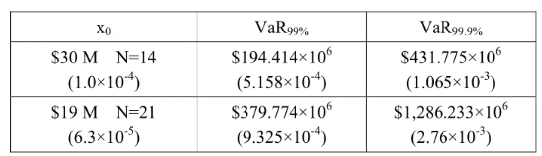
Table A3: VaR99% and VaR99.9%

x0 VaR99% VaR99.9% $30 M N=14 (1.0×10-4) $194.414×106 (5.158×10-4) $431.775×106 (1.065×10-3) $19 M N=21 (6.3×10-5) $379.774×106 (9.325×10-4) $1,286.233×106 (2.76×10-3)

We notice that the results are very different from those estimated in Tables 7 and 8 from the Pareto distribution. The latter are very high for both threshold and different confidence level of the VaR. This confirms our expectation that the Pareto has heavier tail compared to the lognormal distribution. The use of the Pareto for the tail modeling is more precise and rigorous. The lognormal would, in fact, under evaluate the VaR and the operational risk capital.

Figure 1