Meucci : SYMMYS; Kepos Capital
Ardia : Université Laval, Faculté des sciences de l’administration, Département de finance, assurance et immobilier;
et CIRPÉE
Keel : Aeris Capital AG
Cahier de recherche/Working Paper 13-11
Fully Flexible Views in Multivariate Normal Markets
Attilio Meucci
David Ardia
Simon Keel
Abstract:
The Entropy Pooling approach in Meucci (2008) is a versatile, general framework to
process market views in portfolio construction and generalized stress-tests in risk
management. Here we present an efficient algorithm to implement Entropy Pooling with
fully general views in multivariate normal markets.
Then we discuss two applications. First, we use normal Entropy Pooling to estimate a
market distribution consistent with the CAPM equilibrium, which improves on the
“implied returns” a-la-Black and Litterman (1990) and can be used as the starting point
for portfolio construction. Second, we use normal Entropy Pooling to process ranking
signals for alpha-generation.
Keywords: Portfolio construction, tactical allocation, Entropy Pooling, Kullback-Leibler,
Black-Litterman, equilibrium prior, portfolios from sorts, ranking, alpha, signals, factor
models, risk management
1
Introduction
The combination of subjective views on the market within a prior risk model to compute an optimal allocation that incorporates the views is one of the main challenges in quantitative portfolio construction. Similarly, embedding stress-tests in a risk model in a statistically sound way is key to a healthy risk management process.
The generalized Bayesian approach "entropy pooling" (EP) is a general, flexible framework to process views and generalized stress-tests.
The general theoretical framework for EP was laid out in Meucci (2008). EP combines an arbitrary market model, which is referred to as the "prior" and fully general views or stress-tests on the underlying market. The output is a distribution, referred to as the "posterior", which incorporates all the inputs and which can be used for risk management and portfolio optimization. In EP, the posterior is obtained by warping the prior distribution so that the views are fulfilled, in such a way that the prior is minimally distorted. Specifically, the posterior distribution minimizes the entropy relative to the prior, which is the natural measure of discrepancy between two distributions.
The EP framework can be implemented in two ways: non-parametrically, by representing the prior and the posterior in terms of a scenarios-probabilities pair; and parametrically, by making parametric assumptions on the prior and the posterior.
The nonparametric implementation of EP was studied in the original article Meucci (2008) and further extended to handle views on tail risk in Meucci, Ardia, and Keel (2011). The non-parametric approach is very flexible, but subject to the curse of dimensionality. Therefore, it is most effectively applied in risk management contexts, see Meucci (2010).
The parametric implementation of EP was studied in the original article Meucci (2008) under the normal assumption with views set as equalities on expectations and covariances. Under these special types of views, the posterior can be computed analytically.
In this article we study the parametric implementation of EP in normal markets, but with more general views. To compute the posterior, we propose an efficient numerical approach. First, we impose structure on the correlations, thereby increasing the statistical efficiency of our estimates. Second, we compute analytically the gradient of our objective function, namely the relative entropy with the prior, thereby speeding the convergence of our numerical approach. Third, we feed our inputs into an interior point optimizer.
Our framework, namely normal EP with general views, allows us to address a variety of problems. In particular, we discuss two applications.
The first application is the estimation of a market distribution consistent with equilibrium. Such equilibrium estimate is the starting point of portfolio construction in Black and Litterman (1990). In the original paper a covariance of returns is estimated and the "implied" expected returns are then computed ac-cordingly. However, these expected returns are substantially different from their historical counterparts. This issue has been addressed by Levy and Roll (2010)
by simultaneously computing implied expected returns and implied volatilities. Normal EP with general views computes at the same time implied expected returns, implied volatilities and implied correlations, thereby obtaining a closer distribution to the empirical observations.
The second application of the normal EP framework is the extraction of ranking signals for alpha-generation. In the standard approach, discussed e.g. in Grinold and Kahn (1999), the expected return of all the securities in a given market is set proportional to the z-score of a given predictive signal. However, assuming the expected return proportional to the z-score imposes spurious infor-mation in the optimization process. Almgren and Chriss (2006) first addressed this issue, obtaining expected returns that do not overly spurious information. However, their solution does not take empirical data into account. EP effectively estimates ranking-consistent expected returns that do not impose spurious in-formation and at the same time starts from the empirical observations. The case study in Meucci (2008) addresses the low-dimensional case non-parametrically. The present normal EP framework overcomes the curse of dimensionality in large markets.
We emphasize that the multivariate normal specification for the risk drivers that lies at the foundation of our approach is by no means restricted to model normal returns. By applying non-linear pricing functions to the drivers, the normal specification is suitable to model for instance highly skewed markets of options, see Meucci (2009).
The remainder of this article is organized as follows. In Section 2 we review the original general EP framework. In Section 3 we discuss the normal EP implementation. In Section 4 we show how to use normal EP to specify the equilibrium prior. In Section 5 we illustrate how to use normal EP to process ranking signals for portfolio construction.
Fully documented code is available at www.symmys.com/node/160.
2
Review of Entropy Pooling
In this section we draw from Meucci (2008), please refer to that publication for more details.
EP proceeds in three main steps. The first step of EP is the estimation of a "prior" distribution for a set of N risk drivers X ≡ (X1, . . . , XN) in the market,
as represented by its pdf, which we denote by f
X ≡ (X1, . . . , XN) ∼ f. (1)
The risk drivers are any set of random variables that fully determine the secu-rities P&L, such as implied volatility surfaces, returns, etc.
The second step of EP is expressing the views or stress-tests V. These are statements on expectations, correlations, tail risk conditions, etc. that we want the yet to be defined posterior distribution to satisfy. Therefore, views and stress-tests V are constraints on the posterior. We denote that a generic
distribution f satisfies these constraints as follows
f ∈ V. (2)
The third step of EP is the computation of the posterior distribution f for the risk drivers, which incorporates the views stress-tests V. To compute the posterior, first we introduce the relative entropy, a measure of the similarity of a distribution f with respect to a reference distribution, in our case the prior f
E(f|f) ≡ Z
f (x) lnf (x)
f (x)dx. (3)
Then we define the posterior f as the one distribution which is the most similar to the prior f , but at the same time, unlike the prior, satisfies the views V. Therefore, we define the posterior as follows
f ≡ argmin
f∈V E(f|f).
(4)
The posterior distribution f is then used as input to an optimizer to compute the optimal portfolios that incorporate the views V, or to compute summary statistics that reflect the stress-tests V for risk management purposes.
EP can be implemented in two ways: non-parametric and parametric. In the non-parametric approach the prior f is represented in terms of a large number S of joint scenarios for the risk drivers and the associated probabilities {x1,s, . . . , xN,s; ps}s=1,...,S. Then the posterior (4) is represented by the same
scenarios with a new set of probabilities {x1,s, . . . , xN,s; ps}s=1,...,S defined as
follows
p ≡ argmin
p∈V E(p|p),
(5)
where with minor abuse we let E(p|p) ≡PSs=1psln(ps/ps) denote the discrete
counterpart of the relative entropy (3). As it turns out, for several types of views the optimization (5) can be transformed in an instance of linear programming with a low number of variables, and thus it can be efficiently solved numerically. In the parametric approach, all the distributions belong to a given parametric class, i.e. f ≡ fθ, where the parameters θ span a set of values Θ. In particular,
the prior is represented by fθ and the posterior (4) becomes
fθ≡ argmin θ∈Θ fθ∈V E¡fθ|fθ ¢ . (6)
A special case of the parametric approach is the normal assumption
fµ,σ2(x) = (2π)− N
2 |σ2|−12e−21(x−µ)0σ2 −1(x−µ), (7)
where µ is a N × 1 vector of expectations and σ2 is a N × N covariance
symmetric and positive definite, which we denote by σ2
 0. Accordingly, under normality the parametric problem (6) becomes
¡ µ, σ2¢≡ argmin σ2Â0 µ,σ2 ∈V E¡µ, σ2|µ, σ2¢, (8)
where the relative entropy between two normal distributions can be computed explicitly and reads
2E(µ, σ2|µ, σ2) = tr(σ2σ2−1) − ln |σ2σ2−1| + (µ − µ)0σ2−1(µ − µ) − N. (9)
The normal EP problem (8) can be solved analytically when the views are equality statements on expectations E {aX} ≡ ξ and covariances Cov {bX} ≡φ2,
or
V : aµ ≡ ξ, bσ2b0≡ φ2. (10)
Then the solution of (8)-(10) reads
µ = µ + σ2a0(aσ2a0)−1¡ξ − aµ¢ (11)
σ2 = σ2+ σ2b0[(bσ2b0)−1φ2(bσ2b0)−1
− (bσ2b0)−1]bσ2. (12)
It is immediate to check that the posterior¡µ, σ2¢satisfies the views (10).
3
Normal EP with fully flexible views
Here we address the parametric implementation of EP under normality (8), with fully flexible views V beyond (10). In this case, the solution must be computed numerically.
To this purpose, we impose that the covariances be of "low rank + diagonal" type
σ2
≡ bb0+ δ2, (13)
where b is a N × K matrix, δ is a N × N diagonal matrix, and, in large markets, K ¿ N. With the parametrization (13), the EP problem (8) becomes
¡
µ, b, δ¢≡ argmin
µ,b,δ∈VE
¡
µ, bb0+ δ2|µ, σ2¢. (14)
The normal EP optimization (14) presents palatable statistical and numerical features.
From a statistical perspective, the "low rank + diagonal" parametrization of the normal distribution is fully determined by a relatively small number N (K + 2) of parameters θ ≡ (µ, b, δ), instead of the large number N (N + 3) /2 of parameters in the full-blown specification θ ≡ (µ,σ2). The structure imposed
on the correlations by the limited number of parameters substantially enhances the statistical efficiency of the estimates in large dimensional markets.
From a numerical point of view, the parsimonious parametrization θ ≡ (µ, b, δ) is unconstrained, as the parameters can freely range in the space Θ ≡
RN × RN×K × RN. Instead, in the full specification θ ≡ (µ,σ2) the matrix
σ2 is constrained to be symmetric and positive definite. Furthermore, we can
enhance the computational efficiency of the optimization by feeding the analyt-ical expression of the gradient in the interior point algorithms. Indeed, in the technical appendix, we obtain the following results
∂ ∂µE ¡ µ, bb0+ δ2|µ, σ2¢ = ¡µ − µ¢0σ2−1 (15) ∂ ∂δE ¡ µ, bb0+ δ2|µ, σ2¢ = 2 diag¡σ2−1− σ2−1¢δ (16) ∂ ∂bn,kE ¡ µ, bb0+ δ2|µ, σ2¢ = 2PN m=1(σ2−1− σ2−1)n,mbm,k, (17)
where all the high-dimensional inverses σ2−1 and σ2−1 are easily obtained
ana-lytically in terms of a low-cost, low-dimensional inverses as follows
σ2−1 = δ−2− δ−2b¡b0δ−2b + i K
¢−1
b0δ−2, (18)
where iK is K × K identity matrix.
The parsimonious number of entries N (K + 2) in the parameters (µ, b, δ), the fact that the parameters span the unconstrained set Θ ≡ RN×RN×K×RN,
the analytical expression of the gradient (15)-(17) and the analytical inversion (18) makes it possible to converge efficiently to the optimal solution¡µ, b, δ¢in the optimization (14) by means of off-the-shelf interior point algorithms. We proceed to show this in two case studies.
4
Case study: the equilibrium prior
In our first case study we use the normal EP framework with general views to determine the equilibrium distribution that lies at the foundation of the portfolio construction approach in Black and Litterman (1990).
Under some assumptions on the market distribution and the preferences of the investors, the capital asset pricing model purports that the market capital-ization portfolio wM C is linked to the distribution of the market returns by the
identity
E {R} − γCov {R} wM C≡ 0, (19)
where γ > 0 is a risk aversion parameter.
For portfolio construction purposes, the condition (19) guarantees that, in the absence of specific views, a mean-variance optimization yields the portfo-lio wM C. However, the condition (19) is not satisfied empirically by sample
estimates of the expectations and the covariances.
To enforce (19), Black and Litterman (1990) propose a two-step approach. First, a covariance matrix Cov {R} is fitted to empirical observations by means of standard techniques such as exponential smoothing or maximum likelihood; then the equilibrium constraint (19) is solved for the expectations E {R}. This
generates the so-called "implied expected returns". The implied expected re-turns are consistent with equilibrium, but can differ substantially from the true expected values, because no attempt is made to fit jointly covariances and ex-pectations to the observed data.
To address this issue, Levy and Roll (2010), propose to fit a correlation ma-trix bρ2to empirical observations and then ensure that the equilibrium constraint
(19) is satisfied by modifying both the expectations and the variances. More precisely, the authors introduce a distance D between the sample estimates of the expectations and the standard deviations ¡µ, σ¢ and the yet to be defined parameters (µ, σ) as follows D¡µ, σ; µ, σ¢≡ (α ° ° ° °µ − µσ ° ° ° ° 2 + (1 − α) ° ° ° °σ − σσ ° ° ° ° 2 )12, (20)
where k·k denotes the standard Euclidean norm, the division is meant entry-by-entry, and the authors set α ≡ 0.75. Then the authors minimize D with respect to (µ, σ)
(µ, σ) ≡ argmin
µ,σ∈V D
¡
µ, σ; µ, σ¢, (21)
where the equilibrium constraint (19) now reads1
V : µ − γ diag (σ) bρ2diag (σ) w
M C ≡ 0. (22)
Unlike in Black and Litterman (1990), the parameters (µ, σ) are statistically indistinguishable from the sample estimates¡µ, σ¢and thus equally acceptable from an estimation perspective. Furthermore, they give rise to better trading strategies, see Ni, Malevergne, Sornette, and Woehrmann (2011).
To further improve the estimation of the equilibrium distribution we can use our normal EP framework. Accordingly, we replace the Euclidean distance minimization (21) with the relative entropy minimization (14), which we report
here ¡
µ, b, δ¢≡ argmin
µ,b,δ∈VE
¡
µ, bb0+ δ2|µ, bb0+ δ2¢, (23) where the equilibrium constraint (19) now becomes the following view
V : µ − γ¡bb0+ δ2¢wM C ≡ 0. (24)
The EP equilibrium estimates µ and σ2 ≡ bb0+ δ2 improve on the
previ-ous approaches in three directions. First, EP replaces the somewhat arbitrary Euclidean distance between sample and equilibrium estimates with relative en-tropy, a statistically sound measure of discrepancy between distributions. Sec-ond, EP simultaneously adjusts not only expectations and variances, but also correlations. Third, the parsimonious "low rank + diagonal" specification (13) improves the statistical efficiency of the estimates. As a result, the equilibrium parameters¡µ, b, δ¢become less noisy and thus perform better out of sample.
1For simplicity, we drop an additional parameter that enforces beta-neutrality. That
para-meter, along with other constraints mentioned by the authors, can easily be encompassed in our approach.
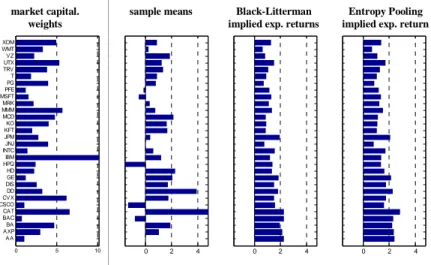
0 5 10 AA AXP BA BAC CAT CSCO CVX DD DIS GE HD HPQ IBM INTC JNJ JPM KFT KO MCD MMM MRK MSFT PFE PG T TRV UTX VZ WMT XOM Weights [%] 0 2 4 Prior [% p.a.] 0 2 4 BL [% p.a.] 0 2 4 EP [% p.a.] market capital. weights
sample means Black-Litterman implied exp. returns
Entropy Pooling implied exp. return
Figure 1: Equilibrium expected returns: Black-Litterman vs. Entropy Pooling
To illustrate the normal EP approach (23)-(24) in practice, we consider a market of N ≡ 30 equities in the Dow Jones Index. For those equities, we consider the time series of the most recent two year of daily returns. Then we fit the empirical prior parameter µ as the sample mean, and σ2
≡ bb0+ δ2 by factor analysis decomposition of the sample covariance with K ≡ 3 hidden factors. Then we determine the equilibrium parameters ¡µ, b, δ¢. Please refer to the code available at at www.symmys.com/node/160 for more details.
In Figure 1 we report the capitalization weights wM C, the sample means µ,
the implied expected returns a-la Black-Litterman µBL≡ γσ2w
M C, and the EP
equilibrium expected returns µ. As expected, the EP parameters µ are more in line with the sample parameters µ than the Black-Litterman parameters µBL.
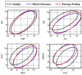
To illustrate the effect of EP on correlations, in Figure 2, we display the location-dispersion ellipsoids that represent geometrically expectations and co-variances, see Meucci (2005). We display the ellipsoids for the sample distribu-tion¡µ, σ2¢, the Black-Litterman equilibrium (µ
BL, σ2) and the EP equilibrium
¡
µ, σ2¢of three stocks.
Notice how the center (expectation), dispersion (variance) and orientation (correlation) of the ellipsoids are modified by the EP approach. Not only the locations are impacted by the views on the tangent portfolio, but the overall covariance structure is modified as well. Again, as expected, the EP parameters are more in line with the sample parameters than the Black-Litterman parame-ters. This illustrates that a constant correlation structure as in Levy and Roll (2010) is restrictive.
-10 -5 0 5 10 -5 0 5 10 AXP BA -10 -5 0 5 10 -5 0 5 10 AA DD -10 -5 0 5 10 -5 0 5 10 BAC CA T -10 0 10 -10 -5 0 5 10 CAT CS CO
Sample Black-Litterman Entropy-Pooling
Figure 2: Equilibrium expected returns: Black-Litterman vs. Entropy Pooling
5
Case study: portfolios from sorts
The second case study addresses portfolio construction with predictive ranking signals. The most standard approach to this problem, popularized by Grinold and Kahn (1999), proceeds as follows.
First, an observable characteristic of a set of N securities, say for instance the price/earnings ratio for stocks, is believed to have predictive power. Then, the N securities are sorted according to the value of the given characteristic. In our example, the stock n = 1 has the lowest price/earnings, the stock n = 2 has the second-lowest price/earnings, and so on, until the stock n = N has the highest price/earnings ratio. Next, an assumption is made that the expected returns of the securities are proportional to their relative ranking
E {Rn} ≡ ˆσn(n − N/2) , n = 1, . . . , N , (25)
where ˆσnis an estimate of the standard deviation of the n-th return; other
spec-ifications, where the expectation is set as proportional to the current historical z-score, are also common, but we do not explore them here for simplicity. Next, the correlation of the securities returns is estimated with standard techniques. Finally, an optimal portfolio is constructed by mean-variance optimization.
The most sensitive step in the above process is setting the expectations proportional to the ranking as in (25). The rationale behind this choice is that, if the signal is truly predictive, a lower ranking should give rise to a lower return
However, the proportional assumption (25) is much more invasive than the rationale (26).
To address this issue, Almgren and Chriss (2006) set the vector of expected returns as the "centroid", i.e. the average among all possible expected returns consistent with the ranking (26). However, the centroid does not depend on the observed empirical data: two completely different sets of securities with the same relative rankings give rise to the same expected returns.
EP allows us to process only the information available from the ranking signal (26) without imposing the spurious proportional structure (25), but at the same time keeping into full account the empirical data. To do so, we start by fitting a prior estimate for the expectations µ and the covariances σ2 ≡ bb0+ δ2
to the data available. Then we compute the posterior parameters by minimizing the relative entropy between the prior and the posterior as in (14), which we report here ¡
µ, b, δ¢≡ argmin
µ,b,δ∈VE
¡
µ, bb0+ δ2|µ, bb0+ δ2¢. (27) In this case, the views are the ranking inequalities (26), which read as follows on the parameters
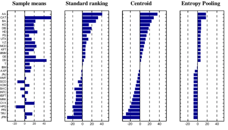
V : µn≤ µn+1, n = 1, . . . , N − 1. (28) The posterior distribution defined by¡µ, b, δ¢can then be used to optimize the portfolio. -20 0 20 40 JPM TRV PFE HPQ CVX MRK MSFT INTC BAC XOM CSCO WMT JNJ AXP IBM T DD GE MMM KFT MCD VZ UTX PG HD DIS KO BA CAT AA Prior [% p.a.] -20 0 20 40 Common [% p.a.] -20 0 20 40 AC [% p.a.] -20 0 20 40 EP [% p.a.]
Sample means Standard ranking Centroid Entropy Pooling
Figure 3: Expected returns for portfolio from sorts
To illustrate how EP applies to building portfolios from sorts, we consider again a market of N ≡ 30 equities in the Dow Jones Index. The prior is constructed from the available sample as in the previous case study. In Figure
3 we report the sample mean returns µ; the expected returns stemming from the standard approach (25); the rescaled centroid; and the EP-ranked expected returns (27)-(28), with the additional long-short constraint PNn=1µn ≡ 0 to better compare the results with the other cases.
As expected, the EP results respect the desired ranking, but at the same time remain as close as possible to the empirical observations summarized by the sample means. Interestingly, though not unexpectedly, the EP expected returns appear to coincide with the centroid when the information from the empirical data is disregarded. For more details, please refer to the code available at www.symmys.com/node/160.
References
Almgren, R., and N. Chriss, 2006, Optimal portfolios from ordering information, Journal of Risk 9, 1—47.
Black, F., and R. Litterman, 1990, Asset allocation: combining investor views with market equilibrium, Goldman Sachs Fixed Income Research.
Grinold, R. C., and R. Kahn, 1999, Active Portfolio Management. A Quan-titative Approach for Producing Superior Returns and Controlling Risk (McGraw-Hill) 2nd edn.
Levy, M., and R. Roll, 2010, The market portfolio may be Mean/Variance effi-cient after all, The Review of Financial Studies 23, 2464—2491.
Meucci, A., 2005, Risk and Asset Allocation (Springer) Available at http://symmys.com.
, 2008, Fully flexible views: Theory and practice, Risk 21, 97—102 Article and code available at http://symmys.com/node/158.
, 2009, Enhancing the Black-Litterman and related approaches: Views and stress-test on risk factors, Journal of Asset Management 10, 89—96 Article and code available at http://symmys.com/node/155.
, 2010, Historical scenarios with fully flexible probabilities, GARP Risk Professional - "The Quant Classroom by Attilio Meucci" December, 40—43 Article and code available at http://symmys.com/node/150.
, D. Ardia, and S. Keel, 2011, Fully flexible extreme views, Journal of Risk (to appear) Article and code available at http://symmys.com/node/159. Ni, X., Y. Malevergne, D. Sornette, and P. Woehrmann, 2011, Robust reverse engineering of cross sectional returns and improved portfolio allocation perfor-mance using the CAPM, Swiss Finance Institute Research Paper No. 11-03.
A
Gradient of relative entropy between normal
distributions
Consider the relative entropy between two multivariate normal distributions 2E(µ, σ2|µ, σ2) = tr(σ2σ2−1) − ln |σ2σ2−1| + (µ − µ)0σ2−1(µ − µ) − N. (29)
Recall the following differentials with respect to the posterior
d ln¯¯σ2σ2−1¯ = tr¯ ¡σ2−1dσ2¢ (30) d tr¡σ2σ2−1¢= tr¡σ2−1dσ2¢ (31) d³¡µ − µ¢0σ2−1¡µ − µ¢´= 2¡µ − µ¢0σ2−1dµ. (32) Then dE =12tr¡(σ2−1− σ2−1)dσ2¢+¡µ − µ¢0σ2−1dµ. (33) We can impose σ2≡ bb0+ δ2. (34)
Then the inversion is fast
σ2−1 = δ−2− δ−2b¡b0δ−2b + i K
¢−1
b0δ−2 (35)
and the differential reads
dσ2= (db)b0+ b(db0) + 2δdδ. (36)
Therefore, we can minimize the relative entropy under linear constraints on σ2
and µ with steepest ascent.
To compute the gradient, we write the first term ("f.t.") in (33) more ex-plicitly as f.t. = tr¡(σ2−1− σ2−1)dσ2¢=P n,m(σ2−1− σ2−1)n,mdσ2n,m =Pn,m(σ2−1− σ2−1) n,m(Pkbm,kdbn,k+Pkbn,kdbm,k+ 2∆n.mδmdδm) =Pu,m,k(σ2−1− σ2−1) u,mbm,kdbu,k (37) +Pn,u,k(σ2−1 − σ2−1) n,ubn,kdbu,k + 2Pn(σ2−1− σ2−1) n,nδndδn = 2Pn,u,k(σ2−1− σ2−1) u,nbn,kdbu,k+ 2Pn(σ2−1− σ2−1)n,nδndδn
=Pu,kqu,kdbu,k+Pnpndδn,
where
qn,k ≡ 2Pm(σ2−1− σ2−1)n,mbm,k (38)