Ravenna: HEC Montréal and CIRPÉE [email protected]
Vincent: HEC Montréal and CIRPÉE [email protected]
Cahier de recherche/Working Paper 14-08
Inequality and Debt in a Model with Heterogeneous Agents
Federico Ravenna
Nicolas Vincent
Abstract:
We propose a DSGE model with income heterogeneity to help discriminate across
competing explanations of the cross-sectional divergence in debt-to-income ratios in US
data. We show that for a DSGE model to be consistent with the data, the divergence in
income growth should not be anticipated and should happen in an economy with low
cost of access to financial intermediation. Differential productivity growth across the top
and bottom-income quantile of the population has a much smaller impact on debt
accumulation by the bottom income-quantile relative to a cross-sectional tax
reallocation.
Keywords: Inequality, debt, DSGE, model
1. Introduction
This paper uses a DSGE model to discuss the impact of changing cross-sectional in-come differentials on the cross-sectional dynamics of consumption and debt. Growing income inequality in the US has been documented by several authors (Krueger, Perri, Pistaferri and Violante, 2008, Lemieux, 2006). Piketty and Saez (2003) find that most of the relative rise in income since 1970 was concentrated at the very top of the income distribution, around 1%. In their influential work, Krueger and Perri (2006) argued that consumption inequality in the US had risen much less than inequality. The divergence in the consumption inequality to income inequality ratio is still the subject of an open debate (Aguiar and Bils, 2011, Attanasio, Hurst and Pistaferri, 2012).
An increase in consumption inequality relative to income inequality should be re-flected in an increase in total debt. In a model with idiosyncratic income shocks, an increase in income volatility leads agents to smooth consumption over time by increas-ing their tradincreas-ing of financial assets. After the US financial crisis, the popular press has often linked the increase in the gross level of household debt to a growing divergence in consumption inequality relative to income inequality.
Household-level data from the Survey of Consumer Finance show that the well-documented rise in household debt over the last 25 years was concentrated below the 90th percentile of the income distribution. Figure 1 illustrates that the cross sectional dispersion in the rise of the debt-to-income ratio occurred not only for mortgage debt, but also for uncollateralized categories of debt.
There is only a limited body of work examining the relation between income inequal-ity, debt inequality and debt accumulation in the context of DSGE models. Iacoviello (2008) builds a model with idiosyncratic income shocks and collateralized borrowing to explain the behaviour of US household debt and consumption-to-wealth ratio. Kumhof and Ranciere (2012) model an economy where income inequality is the result of shocks changing the distribution of revenues between workers and employers, leading to a higher
probability of a financial crisis over time.
We propose a simple DSGE model where heterogeneity in income and consumption is introduced through initial productivity differentials across two groups of agent. Changes in consumption and income inequality are the result of differentiated shocks across the top and bottom quantile of the income distribution. We use our model to assess the implications for consumption inequality and borrowing across income groups in response to an exogenous increase in income inequality. Our model is flexible enough to help discriminate across competing explanations of the cross-sectional divergence in debt-to-income and consumption-debt-to-income ratios in US data. To this end, we consider alternative setups where temporary but long-lived shocks provide an incentive to agents to reallocate consumption intertemporally by using financial markets.
Our results are as follows. First, income inequality driven by cross-sectional differen-tial productivity growth generates much less divergence in the consumption inequality to income inequality ratio than income inequality driven by a cross-sectional tax real-location. The increase in the debt to income ratio for the bottom income group in the case of a tax reallocation is about 100% after 10 years, and only about a fifth in the case of differential productivity growth. This result depends on the fact that productivity differentials also lead to relative price changes for the goods produced by the two groups of agents. In the case of a tax reallocation, the increase in demand by the top income group results in an increase in labor demand for the bottom income group which has only a mild impact on income inequality. Second, a smaller increase in consumption inequality relative to income inequality - and the implied debt increase for the bottom income group - is inconsistent with the hypothesis that the divergence in income growth across groups can be forecasted to increases over time. This would imply that con-sumption for the top income group increases of income, and that indebtedness increases faster for this group relative to the bottom income group. Third, even a mod-est amount of financial intermediation cost reduces dramatically the impact of income
inequality on the divergence in consumption-income inequality and debt accumulation in the bottom income quantile.
2. A Simple Model
Consider an economy populated by two groups of agents, workers and entrepreneurs, with different labor productivity. We label entrepreneurs () the high-productivity group, with an income in the top quantile of the distribution, and workers ( ) the low-productivity group. Variables pertaining the behaviour of entrepreneur-households, or of firms producing output with entrepreneur-hours, are denoted by a ’∗’ superscript. No superscripts is used for variables pertaining to worker-households, or firms using worker-hours. A firm employing labor services () produces output () demanded
by both groups of agents. We define the consumption by entrepreneurs and workers of goods produced by firms using worker-hours respectively as ∗ () () Thus
the index indicates the group supplying the good, while the superscript refers to the group demanding the good. We discuss in the following the equations for the bottom income group only. The top income group behaviour is governed by an identical set of equations.
Worker-households supply labor hours with productivity and consume a basket
of differentiated goods produced by firms using the and groups labor services:
= [( 1 2 1 () −1 +1 2 1 () −1 ] −1 (2.1)
, and indicate the price indices for the aggregate, and goods
consump-tion basket. Preferences for the worker-household are described by the funcconsump-tion:
= ( ln − 1+ 1 + )
budget constraint: + + e+ 2 Ã e !2 ≤ + −1+ e−1+ (2.2)
where is the price of a zero-coupon riskless bond delivering one unit of currency, eis
the amount of asset purchased, is the wage rate, and is a lump sum government
transfer. e−1 indicates the value of the household portfolio of claims. The term 2³ ´2 indicates the real cost of adjusting bond holdings, which is quadratic in the value of the portfolio in terms of consumption units.
Defining the gross nominal interest rate = 1 the gross inflation rate and
the value of bond holdings in consumption units = the optimality conditions are
given by: 0 (1 + ) = ∙ () 1 +1 +10 ¸ (2.3) = 0 (2.4)
Firms specialize in the production of goods (using labor ) or goods (using
labor ∗) employing the technology: () = ()1 Firms are competitive and the
cost minimization problem implies that
=
(2.5)
Since shocks across the two income groups can be asymmetric, there is an incentive for high and low income agents to exchange financial assets. Market clearing on the asset markets implies:
= −∗
Borrowing allows one income group to purchase output for consumption from the sector using as input the labor services of the other income group, in excess of its current
1
income. 2 The budget constraint implies the excess of spending over income for worker-households, denoted is equal to the output sold by entrepreneurs to workers,
net of the value of the output produced by workers and purchased by the top income group. After including the net interest income, we obtain that the change in the net financial asset position for the bottom income group is:
∆ = − −1 = (−1− 1) ∗ (−1 ) − and = ∗ ∗ ∗ − ∗
Our measure of inequality in consumption and in income is given by:
=
∗−
= [ ]
where is total income. We plot the inequality variable in deviations from steady state:
b=
(∗− ) − (∗ − )
= [ ]
Thusb has the interpretation of change in inequality between and ∗ relative to
steady state, as a percentage of the bottom quantile income level.
To measure the evolution of the distance between consumption and income inequal-ity, we build the variable Since at the steady state = the
deviation from steady state of the relative consumption to income inequality is equal to
\ µ ¶ = (− ) − ( − ) = (− )
2An income group can always purchase all the output produced with its labor services, since all the
Thus ³\
´
has the interpretation of the excess change in consumption inequality
relative to income inequality, scaled as a percentage of the steady state income inequality.
3. Dynamics for Inequality and Debt
We consider a parameterization with an elasticity of labor supply 1 equal to 13 and an elasticity of substitution across goods = 15 The parameter is chosen so that a level of borrowing equal to 100% of the income for low-income group results in premium over the riskless interest rate of around 0125 percentage points. We assume in the initial condition entrepreneur-households’ income is 45% higher than the one of worker-households. Consumption inequality in the steady state is identical to income inequality.
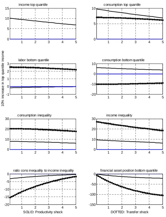
Alternative Transitory Shocks Figure 2 compares the dynamics of the economy for two shocks driving a wedge between income and consumption inequality. The first shock we consider is a temporary increase in the productivity of labor ∗ for the top income group. This shocks interprets the rising income inequality as the result of divergence in productivity growth across income groups.
The second shock we consider is a transfer of resources from the bottom to the top income group. Define the net tax rate ≥ 0 The value of the subsidy to
entrepreneur-households, financed with lump sum taxes on worker-entrepreneur-households, is equal to:
∗ = ∗
∗ ∗
Income in consumption units for the two groups is:
∗ = ∗ ∗ ∗ + ∗= (1 + )∗ ∗ ∗ = ∗ − ∗ ∗
Net financial asset accumulation for the bottom income group is then: ∆= − − ∗ ∗
In this instance, rising income inequality can interpreted as the result of a change in taxation favoring higher than median incomes. It could also be interpreted as the result of the fall in negotiating power for workers with below-median wages, working in sectors open to international competition, relative to workers with above median wages. We scale the two shocks so that income ∗
increases on impact by 10% and the shock
has a half-life of 20 years.
In the case of an increase in productivity for entrepreneur-households, all agents in the economy have an incentive, through the relative price of and goods, to substitute in the consumption basket the relatively inexpensive good for the relatively expensive one . Since the productivity shock raises income only for entrepreneur-households, the bottom income group increases its indebtedness to take advantage of a temporarily lower price of the consumption basket and consumption inequality
increases less than income inequality. After 10 years, the total borrowing of the bottom quantile has increased to about 20% of its income.
The transfer shock provides different incentives to smooth consumption over time. Since the transfer is temporary, both income groups do not change the amount of consumption by the full amount of the income change. For worker-households, income falls by more than consumption, while the opposite is true for entrepreneur-households. However, worker-households also benefit by the demand increase for the good by entrepreneur-households, thus their labor income increases.
The transfer shock generates fall in consumption inequality to income inequality which is about four times as large as the productivity shock, keeping constant the increase in the entrepreneurs’ income. As a consequence, after 10 years the net debt of the bottom income group has increased to 100% of its income.
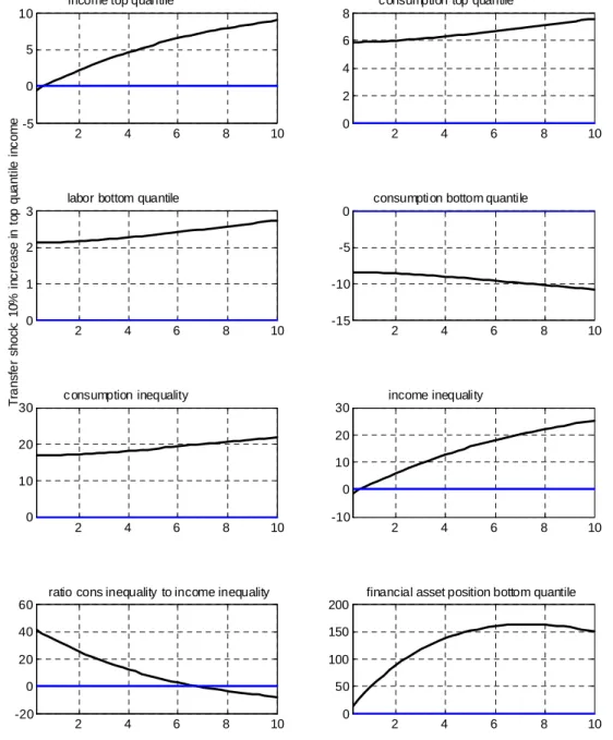
Comparing Expected vs. Unexpected Income Divergence Income inequality in the US has steadily increased starting in the 1980s. We can use our model to analyze the impact of a steady increase in income inequality, where resources are transferred to the top quantile at a higher rate until the transfer peaks at 10% of ∗ after 15 years.
The dynamics resulting from a transfer shock of this sort, shown in figure 3, is inconsistent with the data. Since there are expectations of future increases in income, entrepreneur-households find it optimal to borrow. Thus consumption inequality should increase of income inequality, and the bottom income group would accumulate an enormous credit towards the top income group for the first 10 years of the shock. The model suggests that the data are consistent with a series of unexpected temporary shocks, or with myopic households (in both income groups).
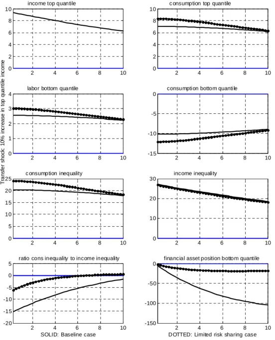
Access to Financial Markets The result of a divergence between consumption in-equality and income inin-equality relies on the possibility of risk sharing through the trad-ing of financial assets. To assess the role of access to the financial market, we consider an economy where the cost of adjusting the portfolio of financial assets is 10 times higher: to carry a debt equal to its steady state income, a worker-entrepreneur would see the quarterly interest rate rise from 1% to 225%
Figure 4 compares the impact of a transfer shock under the high and low cost of ac-cess to financial markets. The increase in the cost of asset trading implies the divergence between consumption and income inequality falls by two thirds. While consumption in-equality by one-fifth, the amount of borrowing by the bottom income group falls by four-fifths. Intuitively, the outstanding debt position cumulates the consumption to income inequality difference over each period, so that borrowing is much more sensitive than consumption inequality to constraints in the possibility of risk sharing.
4. Conclusions
We use a DSGE model with income heterogeneity to help discriminate across competing explanations of the cross-sectional divergence in debt-to-income and consumption-to-income ratios in US data. We show that for a DSGE model to be consistent with the dynamics over time of these variables, the divergence in income growth should not be anticipated, and should happen in an economy with a low cost of access to financial intermediation. As for the driving force of the observed debt-to-income ratio divergence across income groups, our model shows that cross-sectional differential productivity growth has a much smaller impact than a cross-sectional tax reallocation. While our approach describes the evolution of net debt, future models should address the joint evolution of net worth and gross debt across income quantiles, since borrowing for consumption smoothing purposes depends on the amount of borrowing available overall to households, including collateralized mortgages.
References
[1] Aguiar, M. and M. Bils, 2011. Has consumption inequality mirrored income inequal-ity. NBER Working Paper no. 16807.
[2] Attanasio, O., Hurst, E. and L. Pistaferri, 2012. The Evolution of Income, Con-sumption, and Leisure Inequality in The US. NBER Working Paper no. 17982.
[3] Iacoviello, M. 2008. Household Debt and Income Inequality, 1963—2003. Journal of Money, Credit and Banking 40(5), 929-965.
[4] Krueger, D. and F. Perri, 2006. Does Income Inequality Lead to Consumption In-equality? Evidence and Theory. Review of Economic Studies 73(1), 163-193.
[5] Krueger, D., Perri, F., Pistaferri, L. and G.L. Violante, 2008. Cross Sectional Facts for Macroeconomists. Review of Economic Dynamics 13(1), 1-4.
[6] Kumhof, M. and R. Ranciere, 2011. Inequality, Leverage and Crises. CEPR Discus-sion Paper No. 8179.
[7] Lemieux, T., 2006. “Increasing Residual Wage Inequality: Composition Effects, Noisy Data, or Rising Demand for Skill? American Economic Review 96(3), 461-498.
[8] Piketty, T. and E. Saez, 2013. Income inequality in the United States, 1913—1998. The Quarterly Journal of Economics 118(1), 1-41.
[9] Rajan, R., 2010. Fault Lines: How Hidden Fractures Still Threaten the World Econ-omy, Princeton: Princeton University Press.
Figure 4.1: Debt to income ratio from the Survey of Consumer Finances, Board of Governors of the Federal Reserve, 1989 to 2010. Each data points provides the average debt to income ratio for the income quantile.
1 2 3 4 5 0
5 10 15
income top quantile
1 2 3 4 5
0 5 10
consumption top quantile
1 2 3 4 5 -1 0 1 2 3
labor bottom quantile
10 % i n c rea s e i n t o p q u a n ti le i n co m e 1 2 3 4 5 -20 -10 0 10
consumption bottom quantile
1 2 3 4 5 0 10 20 30 consumption inequality 1 2 3 4 5 0 10 20 30 income inequality 1 2 3 4 5 -20 -15 -10 -5 0
ratio cons inequality to income inequality
SOLID: Productivity shock
1 2 3 4 5
-150 -100 -50 0
financial asset position bottom quantile
DOTTED: Transfer shock
Figure 4.2: Impulse response function to a 10% increase in income for the top income quantile. Comparison across a productivity increase for entrepreneur-households rela-tive to worker-households and a lump-sum transfer from bottom to top income group. Log-deviations from steady state in percent. Financial asset position shown as
percent-2 4 6 8 10 -5
0 5 10
income top quantile
2 4 6 8 10 0 2 4 6 8
consumption top quantile
2 4 6 8 10
0 1 2 3
labor bottom quantile
Tr a n s fe r s hoc k: 10 % i n c reas e i n t o p qu a n ti le i n c o m e 2 4 6 8 10 -15 -10 -5 0
consumption bottom quantile
2 4 6 8 10 0 10 20 30 c onsumption inequality 2 4 6 8 10 -10 0 10 20 30 income inequality 2 4 6 8 10 -20 0 20 40 60
ratio cons inequality to income inequality
2 4 6 8 10 0 50 100 150 200
financial asset position bottom quantile
Figure 4.3: Impulse response function to expected growth in income for the top income group up to 110% of steady state income in year 15. Income growth financed through lump-sum transfer from bottom to top income group. Log-deviations from steady state in percent. Financial asset position shown as percentage of steady state income.
2 4 6 8 10 0 2 4 6 8 10
income top quantile
2 4 6 8 10 0 2 4 6 8 10
c onsumption top quantile
2 4 6 8 10 0 1 2 3 4
labor bottom quantile
Tr a n sf e r shoc k: 10 % i n c rease i n t o p qu a n ti le i n c o m e 2 4 6 8 10 -15 -10 -5 0
consumption bottom quantile
2 4 6 8 10 0 5 10 15 20 25 c onsumption inequality 2 4 6 8 10 0 10 20 30 income inequality 2 4 6 8 10 -20 -15 -10 -5 0 5
ratio cons inequality to income inequality
SOLID: Baseline case
2 4 6 8 10
-150 -100 -50 0
financial asset position bottom quantile
DOTTED: Limited risk sharing case
Figure 4.4: Impulse response function to a 10% increase in income for the top quantile. Income growth financed through lump-sum transfer from bottom to top income group. Comparison of baseline case and high cost of asset trading case. Log-deviations from steady state in percent. Financial asset position shown as percentage of steady state income.