Size, Book-to-Market Ratio and Macroeconomic News

Texte intégral

(1)Cahier de recherche/Working Paper 10-33. Size, Book-to-Market Ratio and Macroeconomic News. Tolga Cenesizoglu. Septembre/September 2010. Cenesizoglu : Department of Finance, HEC Montreal, 3000, Chemin de la Cote-Sainte-Catherine, Montreal (Quebec) Canada H3T 2A7; phone : +1 514 340-5668; and CIRPÉE tolga.cenesizoglu@hec.ca I would like to thank Allan Timmermann for his helpful comments on earlier versions of this paper. I also benefited from conversations with Bruce Lehmann, Richard Carson, Rossen Valkanov, Jun Liu, Jason Murray, Jonathan Smith, Pascal François and Lars Stentoft. I would also like to thank my discussant at Northern Finance Association Meetings, Eastern Finance Association Meetings, Financial Management Association Meetings. Earlier versions of this paper were circulated under the title “Asymmetries in the Reaction of Stock Prices to Macroeconomic News”..

(2) Abstract: Little is known about the reactions of daily returns on portfolios with different characteristics to unexpected changes in macroeconomic conditions. This paper fills this void by analyzing the reactions of daily returns on portfolios formed on size and book-tomarket ratio to news about a wide range of macroeconomic variables. Returns on different portfolios not only react to different news but also react differently to the same news. Reactions of portfolios to macroeconomic news also change over the business cycle. Results are strongest for news about employees on nonfarm payrolls in expansions. Both at daily and monthly frequencies, large and growth firms react differently to employment news from small and value firms in expansions but not in recessions. Differences in the sensitivities of expected future cash flows to employment news in expansions can help explain differences in the observed reactions. Keywords: Macroeconomic News, Employees on Nonfarm Payrolls, Business Cycle, Cash Flow, Discount Rate, Return Decomposition JEL Classification: G10, G12, G14.

(3) 1. Introduction. The relation between returns, fundamentals, such as cash flows and discount rates, and unexpected changes in macroeconomic conditions is of central importance to financial decision making. Investors need to know how returns and fundamentals are affected by unexpected changes in macroeconomic conditions for portfolio allocation, risk management and asset pricing purposes. Furthermore, macroeconomic variables might contain important information about investors’ future consumption. The intertemporal capital asset pricing model (ICAPM) of Merton (1973) suggests that state variables that predict time variation in future investment opportunity sets should be included as factors in asset pricing models. Among the most important candidates for state variables in multi-factor asset pricing models are innovations in macroeconomic variables such as GDP or consumption growth, employment rate and shortterm interest rates. Hence, it is not surprising to find a relatively large literature analyzing the low-frequency (monthly or annual) relation between the cross-section of returns and macroeconomic variables.1 However, the literature focuses mostly on an aggregate index rather than individual stocks or portfolios formed on certain firm characteristics when analyzing the high-frequency (intra-day or daily) relation.2 This paper fills this void by analyzing the high-frequency relation between returns on portfolios with different characteristics and a wide range of macroeconomic variables. Specifically, we analyze whether daily returns on portfolios of firms with different market capitalizations and book-to-market (BM, hereafter) ratios react to different types of macroeconomic news or react differently to the same macroeconomic news. A closely related literature argues that differences in the sensitivities of fundamentals to changes in aggregate conditions can help explain differences in the cross-section of returns. Due to the low-frequency nature of fundamentals such as cash flows, this strand of the literature focuses on the low-frequency relation between firm- or portfolio-level fundamentals and aggregate conditions. For example, Bansal, Dittmar, and Lundblad (2005) analyze the relation between cash flows and aggregate consumption at quarterly frequency whereas Campbell, Polk, and Vuolteenaho (2010) analyze the effect of the market’s cash flow and discount 1. The consumption CAPM of Breeden (1979) and the human capital augmented CAPM of Campbell (1996) and Jagannathan and Wang (1996), and the conditional versions of these models discussed in Lettau and Ludvigson (2001) are prominent examples of multi-factor asset pricing models with macroeconomic variables. Closely related to these models are the multi-factor asset pricing models of Fama and French (1993) and Campbell and Vuolteenaho (2004a) where priced risk factors are of financial nature rather than macroeconomic. 2 A partial list of studies analyzing the reaction of stock prices to macroeconomic announcements includes Pearce and Roley (1985), McQueen and Roley (1993), Flannery and Protopapadakis (2002), Bomfim (2003), Guo (2004), Bernanke and Kuttner (2005), Boyd, Hu, and Jagannathan (2005) and Andersen, Bollerslev, Diebold, and Vega (2007). Most of these studies focus on the reaction of an aggregate market index rather than individual stocks or portfolios with different characteristics with the exceptions of Guo (2004) and Bernanke and Kuttner (2005) who analyze the reaction to unanticipated changes in the target rate. Bernanke and Kuttner (2005) analyze the reactions of industry portfolios whereas Guo (2004) analyzes the reactions of portfolios formed on size. After the first draft of this paper was circulated, we became aware of Gosnell and Nejadmalayeri (2009). The authors analyze the reactions of three Fama French factors to news about macroeconomic variables. However, they analyze neither the reactions of portfolios nor the possible sources of the observed reactions.. 1.

(4) rate news on both cash flows and discount rates of portfolios formed on BM ratio at monthly and annual frequencies.3 In this paper, we also provide empirical evidence on the low-frequency relation between portfolio-level fundamentals and aggregate conditions. However, our goal is different from that of the existing literature as we analyze the effect of employment news on fundamentals in order to better understand the differences in the observed reactions of portfolio returns to news about this variable. Using survey data on consensus forecasts and data on federal funds futures to capture the expected part of macroeconomic announcements, we first estimate the reactions of daily returns on the ten size- or BM-sorted portfolios to 21 different macroeconomic variables. Portfolios with different characteristics not only react to news about different variables but also react differently to news about the same variable. For example, large and growth firms, on average, react negatively to higher than expected employees on nonfarm payrolls whereas the reactions of small and value firms are insignificant. Moreover, these differences are statistically significant. When we distinguish between different phases of the business cycle as in McQueen and Roley (1993) and Boyd, Hu, and Jagannathan (2005), we find that our results are mainly due to the significant reactions of stock returns in expansions rather than in recessions. Several tests suggest that our empirical results are robust to using alternative definitions of the news variable, control variables, subsample periods and alternative empirical specifications. We then turn our attention to the effect of employment news, one of the most important macroeconomic variables, on fundamentals at the monthly frequency in order to analyze the possible sources for the differences in the observed reactions. First of all, we establish that firms with different characteristics continue to react differently to news about employees on nonfarm payrolls at the monthly frequency. Specifically, large and growth firms continue to react negatively to higher than expected employment numbers in expansions whereas their reactions continue to be insignificant in recessions. On the other hand, the reactions of small and value firms become positive and significant in expansions and remain insignificant in recessions. Secondly, using the return decomposition approach of Campbell and Shiller (1988a), we decompose unexpected monthly returns on these portfolios into their fundamentals to analyze the possible sources for the observed reactions. In line with findings of McQueen and Roley (1993) and Boyd, Hu, and Jagannathan (2005), we find that the negative reaction of large firms in expansions is mainly due to an increase in the discount rate following higher than expected employment numbers in expansions. On the other hand, the positive reactions of small and value firms in expansions are mainly due to an increase in their expected future cash flows following higher than expected employment numbers. More importantly, we find that the 3. Also related to this strand of the literature are Gertler and Gilchrist (1994) and Xing and Zhang (2004). Gertler and Gilchrist (1994) analyze the effect of monetary policy on the fundamentals of small and large firms over the business cycle whereas Xing and Zhang (2004) analyze the effect of negative business cycle shocks on the fundamentals of growth and value firms.. 2.

(5) significant differences in the reactions of small-value firms and large-growth firms in expansions are mainly due to different sensitivities of their cash flows to employment news in expansions. Finally, as a robustness check, we analyze the actual relation between dividend growth rates and actual changes in employment numbers as in Boyd, Hu, and Jagannathan (2005). We find the cash flows of small and value firms to be more sensitive to changes in employment numbers, similar to the findings of Bansal, Dittmar, and Lundblad (2005) and Campbell, Polk, and Vuolteenaho (2010). The rest of the paper is organized as follows. In Section 2, we describe the data sets used in our empirical analysis. In Section 3, we present our empirical results on the reactions of daily returns to macroeconomic news. Section 4 takes a closer look at the reactions of returns to employment news. We analyze the possible sources of the observed reactions in Section 5. We discuss our empirical results in relation to the existing literature in Section 6. We provide concluding remarks in Section 7.. 2. Data. In this section, we describe the methods and data sets used to capture the market’s expectations about macroeconomic variables. We also briefly describe the data set on daily returns. We obtain data on real-time macroeconomic variables as first reported and the market’s expectations about these variables from the Money Market Services International (MMS, hereafter) data set.4 For the Employees on Nonfarm Payrolls, one of the most important variables, the announcement days are available to us from the Federal Reserve Bank of Philadelphia since 1965. However, the survey expectations for this variable from the MMS data set are only available starting 1985. To extend our data set and analyze the robustness of our results to using alternative definitions of news and different sample periods, we also use an econometric model as in Boyd, Hu, and Jagannathan (2005) to obtain the market’s expectations about this variable. We discuss the details of this econometric approach in Section 4. To distinguish between the expected and unexpected components of changes in the Federal Funds Target Rate, we use daily data on 30 Day Federal Funds Futures traded on the Chicago Board of Trade (CBOT).5 4 The benchmark weekly MMS survey has been conducted since 1980 and is the most complete history of real-time data as well as the market’s consensus forecast of US macroeconomic variables. Every Friday, except holidays, MMS surveyed approximately 40 economists, market strategists from major commercial banks, top brokerage houses, consulting firms, some major universities and some fund management companies by telephone, fax or e-mail for their forecasts of the upcoming week’s announcements. The survey results are released around 1:30 P.M. EST (Eastern Standard Time) every Friday. The MMS data and its description are available from Haver Analytics. 5 The data on 30 Day Federal Funds Futures is available from Datastream. The contracts are cash settled against the average daily Fed funds overnight rate where the average is calculated over all calendar dates of the delivery month by carrying the rate from the last business day for weekends and holidays. The implied Federal Funds Target Rate is 100 minus the price quote. Our data set for news about the Federal Funds Target Rate begins with the rate cut of 25 basis points on July 6, 1989 and ends with the Federal Open Market Committee (FOMC) meeting on December 16, 2009 when the rate was kept constant.. 3.

(6) Following Kuttner (2001) and Bernanke and Kuttner (2005), we define the announcement days for the Federal Funds Target Rate as the union of the (FOMC) meeting days and the unscheduled announcement days where the FOMC decided to change the rate unexpectedly. We use daily returns between February 1965 and December 2009 on the ten value-weighted portfolios sorted with respect to either size (market equity) or book-to-market ratio (book equity/market equity) available to us from Ken French’s web site.6 Although daily returns on these portfolios are available to us since July 1963, we restrict our attention to the sample period for which we observe the announcement days for Employees on Nonfarm Payrolls. The availability of consensus forecasts and realized values differ across macroeconomic variables because the MMS did not survey participants about a macroeconomic variable prior to the start date of availability presented in Table 1. This table summarizes several features of our macroeconomic news data set such as the number of news observations available, the reporting agency, the start and end date of availability, the announcement release time and summary statistics for standardized news.7 [INSERT TABLE 1 HERE] Following the previous literature (Balduzzi, Elton, and Green (2001), Andersen, Bollerslev, Diebold, and Vega (2003) and Andersen, Bollerslev, Diebold, and Vega (2007)), we use the standardized news defined as the difference between the actual released announcement and the consensus median market forecast from the MMS divided by the sample standard deviation of this difference. Specifically, the standardized news 6. One can also use intraday data to capture the effect of macroeconomic news more precisely during a shorter time period around an announcement (see Andersen, Bollerslev, Diebold, and Vega (2007)) or to analyze the effect of announcement time during a trading day (see Greene and Watts (1996)). Although, intraday data would be suitable to analyze the reaction of returns on an individual stock or a portfolio, we choose to use daily data for several reasons. First of all, it would be relatively difficult to compare the reaction of returns on different portfolios due to nonsynchronous trading during a relatively shorter period of time. Secondly, it is relatively difficult to construct an intraday data set of returns on different portfolios due to market microstructure issues whereas daily data is readily available. Finally, most studies analyzing the reaction of returns on an aggregate index to macroeconomic news also use daily data on returns. (e.g. Flannery and Protopapadakis (2002), Boyd, Hu, and Jagannathan (2005)) 7 Following Andersen, Bollerslev, Diebold, and Vega (2003), we first group macroeconomic variables into three main groups with respect to their announcement frequency: quarterly, monthly and six-week. We then group monthly variables into 6 subgroups: Real Activity, Consumption, Investment, Net Exports, Prices, and Forward-Looking. There are several problems with matching an announcement day of a macroeconomic variable to a trading day. If there is an announcement on a non-trading day, instead of losing that observation, we assume that the effect of that announcement would be realized in the first trading day following the announcement. For example, the stock market is closed on Good Fridays whereas it is a regular business day for most reporting agencies. Hence, we assign those announcements made on Good Fridays to the first Monday following the announcement. The second problem is due to the release of two announcements of the same macroeconomic variable on the same day. This is not very common in our data set and generally happens due to a delay in the release on the previous announcement day. We take a simple average of the unexpected parts of the delayed and the current announcements released on that day. Furthermore, there are announcement days in our sample for which we are not able to calculate the news variable due to either a missing forecast or a missing real-time value. We treat such trading days as non-announcement days even though we know that an announcement for a particular macroeconomic variable was released on those trading days.. 4.

(7) for macroeconomic variable j on the announcement day t, Sj,t , is defined as Sj,t =. Aj,t − Fj,t σ ˆj. (1). where Aj,t and Fj,t are, respectively, the actual released value and the consensus market expectation obtained as the median forecast from the MMS data set for the macroeconomic variable j on the announcement day t. The difference, Aj,t − Fj,t , is the news (non-standardized) variable and σ ˆj is the in-sample standard deviation of the news variable calculated using all available data for the macroeconomic variable j, i.e. p c j,t − Fj,t ). The standardization of the news allows us to compare the effect of different σ ˆj = var(A macroeconomic variables with different units of measurement. The unexpected part of an announcement about the Federal Funds Target Rate can be captured from the change in the price of the 30 Day Federal Funds Futures due to the announcement. Hence, we define news about the Federal Funds Target Rate as S21,t =. D 0 (f 0 − fm,t−1 ) D − d m,t. (2). where m denotes the corresponding month for the announcement day t and D is the number of calendar 0 is the price of the spot-month futures contract on the announcement day t in month m days in month m. fm,t 0 and fm,t−1 is the price of the same futures contract on the day before the announcement. We refer the reader. to Kuttner (2001) and Bernanke and Kuttner (2005) for further details on this approach.8 We should note that news about the Federal Funds Target Rate differs from news about other variables in two ways. First of all, news is defined using data on futures rather than data on expectations from the MMS survey. Secondly, some announcement periods were not known in advance by the market participants whereas announcements about other variables are generally scheduled and the timing is known to the public in advance.9 Table 1 also presents summary statistics for the standardized news for each macroeconomic variable in our data set. The standardized news for most macroeconomic variables has a mean around zero confirming the findings of the previous literature on the unbiasedness of the MMS forecasts. There is no macroeconomic variable with a standardized news that has a mean significantly different from zero. However, one should note that there are few variables such as the Federal Funds Target Rate that might have possible outliers. 8. For the time period analyzed by Kuttner (2001), the expected and unexpected components of changes in Federal Funds Target Rate in our data set are identical to those reported in Table 2 of Kuttner (2001). 9 Especially prior to 1994, the announcement days for the Federal Funds Target Rate were not regularly scheduled. Even after 1994, when the Federal Reserve Board adopted the policy of officially announcing its decision on the target rate, there are few unscheduled announcements between the official Federal Open Market Committee meeting days.. 5.

(8) 3. The Reaction of Portfolio Returns to Macroeconomic News. In this section, we first analyze the reactions of returns on the ten size- or BM-sorted portfolios to macroeconomic news where we do not distinguish between different economic conditions. We then turn our attention to the reactions over the business cycle where we distinguish between economic expansions and recessions.. 3.1. The Reaction of Portfolio Returns to Macroeconomic News over the Whole Sample. To analyze the reaction of stock returns to news about macroeconomic variables over the whole sample where we do not distinguish between different states of the economy, we estimate the following linear specification: ri,t = β0,i +. 21 X. β1,ij Sj,t +. j=1. 21 X. β2,ij Ij,t + εi,t. (3). j=1,j6=14. where ri,t is the return on the ith (i = 1, 2, . . . , 10) decile portfolio of the ten size- or BM-sorted portfolios. Sj,t is the news about the macroeconomic variable j on the trading day t described as in Equation (2) for the Federal Funds Target Rate and Equation (1) for other variables. Ij,t is a binary variable that is equal to one if it is an announcement day for the macroeconomic variable j and zero otherwise.10 We assume that Sj,t is zero if t is not an announcement day for the macroeconomic variable j. We opt to use this specification rather than estimating the effect of each macroeconomic variable separately using data only on announcement days for that macroeconomic variable. This specification takes into account the possibility of several announcements on the same day which is common in our data set11 and captures only the effect of the variable of interest by controlling for the possible reaction to other news released on the same day. Furthermore, the announcement day dummy variable, Ij,t , controls for other possible effects of announcement days on returns that are not captured by the surprise variable.12 We estimate the linear specification via seemingly unrelated regressions (SUR) for the ten size-sorted portfolios and the ten BMsorted portfolios. Estimating the coefficients using SUR allows the error terms across different portfolios to be correlated and allows us to test hypotheses on the coefficient estimates of different portfolios.13 10. Export and Import Price Indices are always announced on the same day. Hence, the announcement day dummy variable, Ij,t , during our sample period is identical for these two variables. To avoid the problem of multicollinearity, we arbitrarily choose to drop the dummy variable for the Export Price Index (variable 14). 11 There are 1,483 trading days (13% of our sample) with two or more announcements released. 12 We also estimated the effect of each macroeconomic variable separately using data only on announcement days for that macroeconomic variable. Doing so, we only consider announcement days for a specific macroeconomic variable without controlling for the effect of other macroeconomic variables on returns. We find that the main results discussed in this section on the asymmetries in reactions of different portfolios to macroeconomic news remain unchanged. 13 Due to relatively large number of observations, it is impossible to estimate the specification in Equation (3) for daily returns on the ten size- or BM-sorted portfolios via Generalized Method of Moments (GMM) with heteroscedasticity and autocorrelation consistent (HAC) standard errors. Although the estimation of a simple linear specification is relatively straightforward, the GMM. 6.

(9) Table 2 presents the reactions of returns on the ten size-sorted portfolios to news about macroeconomic variables estimated based on the data set excluding the possible outliers of the target rate news.14 [INSERT TABLE 2 HERE] Here, we discuss the overall significance of the reactions to macroeconomic news before turning our attention to signs of the reactions in the next section when we distinguish between different phases of the business cycle. Different deciles of the size-sorted portfolios react to news about different macroeconomic variables. To identify whether the reactions to a specific macroeconomic news are jointly significant across all size-sorted portfolios, Table 2 also presents the Bonferroni p-values for each macroeconomic variable. These p-values provide a robust and conservative measure of significance across portfolios and allow us to understand whether news about a specific variable reveals important information for the size-sorted portfolios. Based on 10% significance level for the Bonferroni p-values, the size-sorted portfolios react significantly to news about Employees on Nonfarm Payrolls, Retail Sales, Trade Balance and several price indices. Size-sorted portfolios also react significantly to news about other variables such as Hourly Earnings, Consumer Credit, Housing Starts and the Federal Funds Target Rate although the conservative Bonferroni p-values do not identify these variables to be important. Similar to the findings of the previous literature, none of the size-sorted portfolios react significantly to news about macroeconomic variables considered important such as GDP related variables and Industrial Production. A closer look at the reactions of the size-sorted portfolios to news about macroeconomic variables reveals important asymmetries between large and small stocks. The significance of the reactions to news about Employees on Nonfarm Payrolls as measured by the Bonferroni p-values are generally due to the significant reaction of stocks with relatively higher market capitalizations (6th to 10th decile portfolios). On the other hand, the significant reaction to Retail Sales is mainly due to the significant reaction of smaller algorithm fails to converge due to the large number of observations. Hence, in this section, we choose to present the results for the ten size- or BM-sorted portfolios based on SUR estimation. On the other hand, we can estimate the specification in Equation (3) via GMM with HAC standard errors for the first and tenth deciles of the size- or BM-sorted portfolios and a limited number of macroeconomic variables. We discuss the results of this and other robustness checks for the reaction to news about Employees on Nonfarm Payrolls in the next section. 14 To analyze the effect of possible outliers, we include the square of the surprise variables as additional explanatory variables in our empirical specification in Equation (3). If the squared surprise has a significant effect on returns and/or the effect of the surprise variable itself becomes insignificant, we argue that the outliers of that macroeconomic variable might have an impact on our empirical results. We find that the only variable for which the reactions of portfolios are sensitive to possible outliers is the target rate. Bernanke and Kuttner (2005) also argue that the reaction of the aggregate market portfolio to news about the target rate is sensitive to possible outliers. Hence, we choose to present coefficient estimates based on the data set excluding the possible outliers of the target rate news. The last row of each table presents the reaction to target rate news based on the whole sample including outliers. The coefficient estimates of other variables do not change significantly whether we include or exclude outliers of the target rate news. The results based on the whole data set including the outliers for the target rate news are available from the author upon request.. 7.

(10) firms (1st to 6th decile portfolios). Almost all size-sorted portfolios react significantly to news about Trade Balance, several price indices and the Federal Funds Target Rate.. 15. To analyze whether the differences in the reactions of small and large stocks are statistically significant, the last column of Table 2 presents the Wald statistics testing the equality of the reactions of the first and tenth decile portfolios to each macroeconomic news. The only variable for which the reaction of large stocks is significantly different from that of small stocks is the Employees on Nonfarm Payrolls.16 Furthermore, the strength of the reaction to news about this macroeconomic variable (the absolute value of the coefficient estimate) increases almost monotonically with market capitalization. We analyze the differences in the reactions of small and large stocks to a relatively large number of macroeconomic variables. One might argue the fact that searching over a large set makes it more likely that the researcher might find significant results for a smaller set of these variables. For example, at the 10% significance level, we might find that the reactions of small and large stocks are statistically significant from each other by pure chance for 2 of 21 variables analyzed. First of all, Employees on Nonfarm Payrolls is arguably the most important macroeconomic variable, sometimes referred as the “king of announcements”. Secondly, there is also anecdotal evidence in the press that the market closely follows news about this variable. Finally, to avoid any concerns of data mining in our results, the last column of Table 2 also presents the significance level of the equality test based on standard errors corrected via the Bonferroni correction. Our results suggests that the significant difference between the reactions of small and large firms is not possibly due to data mining issues. The difference in the reactions of small and large stocks to news about Employees on Nonfarm Payrolls is not only statistically but also economically significant. On average, a one standard deviation positive surprise in the employment numbers decreases the return on large stocks by 18 basis points. The effect is only 3 basis points and insignificant for the return on small stocks. The difference of 15 basis points between the reactions of small and large stocks is economically significant for daily returns.17 Table 3 presents the reactions of the ten BM-sorted portfolios to news about macroeconomic variables. 15. Monetary policy decisions, e.g. the raw change in the Federal Funds Target Rate, might have different effects on portfolio returns with different characteristics in addition to the news variable. To this extent, we estimated an empirical specification similar to the one in Bernanke and Kuttner (2005) where they estimate a regression of the CRSP-value weighted return on the raw change. In line with their findings, we also find that the raw change in the target rate does not have a significant effect on the portfolio returns. Furthermore, our results on the effect of the news variable about the target rate does not change significantly when we control for the raw change. 16 The reaction of small and large stocks are also significantly different from each other for news about Housing Starts and Federal Funds Target Rate although the overall reaction of size-sorted portfolios as measured by the Bonferroni p-values is not significant. Furthermore, the reaction to the Federal Funds Target Rate is sensitive to possible outliers of this news variable. 17 The interpretation of the reaction to other variables is similar except the Federal Funds Target Rate since it is measured differently than other variables. A one basis points unexpected raise in the target rate significantly decreases the one-day return of large stocks by 2.85 basis points where is it decreases the one-day return on small stocks by 1.39 basis points.. 8.

(11) At the 10% significance level for the Bonferroni p-values, the ten BM-sorted portfolios react significantly to news about Employees on Nonfarm Payrolls, Trade Balance, Housing Starts, Federal Funds Target Rate and several price indices. Several of the BM-sorted portfolios also react significantly to news about Hourly Earnings and Retail Sales although the reactions of all BM-sorted portfolios to news about these variables are not significant as measured by the Bonferroni p-values. [INSERT TABLE 3 HERE] The significant reaction to news about Employees on Nonfarm Payrolls and Core CPI is mainly due to the significant reactions of growth rather than value firms whereas the opposite holds true for news about Export Price Index. The reactions to news variables such as Trade Balance, Housing Starts and the Federal Funds Target Rate are almost uniformly significant across all deciles of the BM-sorted portfolios. More importantly, growth and value firms react significantly different from each other to news about Employees on Nonfarm Payrolls, Retail Sales, Export Price Index and Core CPI.18 However, as for the sizesorted portfolios, the only variable for which this differential reaction is not possibly due to issues related to data mining is the Employees on Nonfarm Payrolls. The strength of the reaction to news about Employees on Nonfarm Payrolls decreases almost monotonically with respect to the BM ratio. Our results on the reactions of the BM-sorted portfolios to news about Employees on Nonfarm Payrolls are also economically large. A one standard deviation positive surprise about Employees on Nonfarm Payrolls, on average, decreases the one-day return on growth stocks by 19 basis points and value stocks by only 3 basis points. The difference of 16 basis points is economically significant for daily returns.. 3.2. Reaction of Portfolio Returns to Macroeconomic News over the Business Cycle. Several previous studies, including McQueen and Roley (1993), Andersen, Bollerslev, Diebold, and Vega (2007) and Boyd, Hu, and Jagannathan (2005), analyze the reaction of S&P 500 returns to macroeconomic news over the business cycle and find that the effect of macroeconomic news on S&P 500 returns differs between economic expansions and recessions. In this section, we analyze the reactions of stock returns on portfolios with different characteristics to macroeconomic news over the business cycle. We use the business conditions index of Aruoba, Diebold, and Scotti (2009) (ADS index, hereafter) 18. Our results on the reaction of portfolios to news about the target rate are sensitive to the possible outliers of this variable. If we estimate the reaction of BM-sorted portfolios using the whole data set including the possible outliers, the reactions of growth and value firms are significantly different from each other. However, this does not hold true when we exclude the possible outliers. We believe that the results are more sensible when we exclude the possible outliers since none of the BM-sorted portfolios except the first decile portfolio reacts significantly to target rate news when we include the possible outliers.. 9.

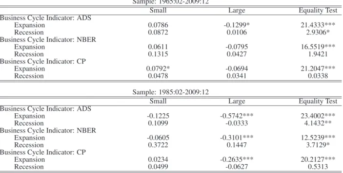
(12) available to us from the Federal Reserve Bank of Philadelphia.19 The ADS index is designed to track economic conditions in real-time with high frequency data. The average value of the ADS index is zero and values greater (smaller) than zero indicate better (worse) than average economic conditions. We choose to use the ADS index since it is available at the daily frequency.20 To analyze the reactions over the business cycle, we estimate the following empirical specification via SUR for ten deciles of the size- or BM-sorted portfolios: exp. rec ri,t = β0,i 1rec,t + β0,i (1 − 1rec,t ) +. 21 X. rec β1,ij Sj,t 1rec,t +. j=1. +. 21 X. rec β2,ij Ij,t 1rec,t +. j=1,j6=14. 21 X. 21 X. exp. β1,ij Sj,t (1 − 1rec,t ). j=1 exp. β2,ij Ij,t (1 − 1rec,t ) + εi,t. (4). j=1,j6=14. where 1rec,t is a dummy variable that is equal to one if the ADS is negative on trading day t and zero otherwise. [INSERT TABLE 4 HERE] We first focus on the reactions of stock returns to news about Employees on Nonfarm Payrolls over the business cycle. First of all, returns on small and value stocks react significantly to news about this variable during periods of good economic conditions even though the overall reaction is insignificant when we do not distinguish between different economic conditions. Secondly, the overall significant reactions of sizeor BM-sorted portfolios based on the Bonferroni p-values are mainly due to their significant reactions in expansions rather than in recessions. Finally and more importantly, the difference in the reactions of smallvalue and large-growth firms to news about Employees on Nonfarm Payrolls is more pronounced during periods of good economic conditions. The strength and robustness of our results about Employees on Nonfarm Payrolls might not be surprising as it is one of the most important macroeconomic variables that the market “watches” closely. However, the sign of the reaction might be relatively counterintuitive as our results suggest that the stock market responds negatively to positive news about employment numbers. In other words, news about improving labor market conditions decreases daily stock returns on size or BM-sorted portfolios. These results are counterintuitive 19. Since the ADS index is updated as data on the index’s underlying components are released, its real time nature is important. In this paper, we use the vintage available as of 14 May 2010. However, one should keep in mind that these values of the index would not have been available to the investors until 14 May 2010, a similar issue faced by NBER recession dates. In the next section, we discuss the robustness of our results to an alternative measure of economic conditions based on the real-time recession probabilities of Chauvet and Piger (2008). 20 We also consider alternative definitions of economic conditions such as dummy variables based on the NBER recession dates and real-time recession probabilities of Chauvet and Piger (2008) which we discuss in further detail below. Our results presented in this section are robust to these alternative definitions of economic conditions.. 10.

(13) as one would expect the stock returns to react positively to news about improving economic conditions. First, we should note that this is not a reflection of the methodology used to capture the unexpected part of an announcement since, as we discuss below, our results are robust to using alternative definitions of employment news and economic conditions. Secondly, we are not the first to report this counterintuitive reaction of stock returns to positive employment news. Our results are consistent with those discussed in McQueen and Roley (1993), Boyd, Hu, and Jagannathan (2005) and Andersen, Bollerslev, Diebold, and Vega (2007). We discuss these results in further detail in Section 6. Briefly, the argument can be summarized as follows. An unanticipated increase in the employment rate during periods of economic expansions may lead to an increase in interest rate expectations with a negative effect on stock prices and an increase in growth expectations with a positive effect on stock prices. However, the interest rate effect dominates the growth rate effect causing stock returns to react negatively to an unanticipated increase in employment numbers. Our results for other macroeconomic variables are broadly consistent with those in McQueen and Roley (1993) and Andersen, Bollerslev, Diebold, and Vega (2007) and can be summarized as follows: 1. Variables such as Hourly Earnings and Core CPI reveal important information about stock returns in expansions but not in recessions. 2. Other variables such as Construction Spending and Hourly Earnings reveal important information about stock returns in recessions but not in expansions. 3. There is also some evidence of significant differences in the reactions of portfolios to news about some other variables such as Core PPI in expansions. On average, stock returns react negatively to higher than expected price levels and target rates in both expansions and recessions. Higher than expected price levels or target rate signal higher than expected discount rates for the cash flows of firms which in turn results in a decreases in stock prices. As in McQueen and Roley (1993), stock returns react negatively to news about improving economic conditions, such as good news about Construction Spending, in expansions. This might be also explained by the larger increase in discount rates relative to the increase in expected future cash flows following news about improving economic conditions in expansions. We discuss this argument in more detail in Section 5.. 11.

(14) 4. The Reaction to News about Employees on Nonfarm Payrolls. For the rest of the paper, we focus on the Employees on Nonfarm Payrolls and refer to it as employment numbers or news. Before proceeding to the possible sources of the reaction, we take a closer look at the reaction of stock returns to news about this variable in this section. We start with analyzing the robustness of our results to using different subsamples as well as alternative definitions of news, economic conditions and portfolios. We then analyze the robustness of our results to including unobserved macroeconomic factors in our empirical specification as control variables. Finally, we also analyze the reaction of stock returns in a multivariate GARCH framework.. 4.1. Alternative Definitions of News, Economic Conditions and Portfolios. As mentioned in Section 2, the announcement days for employment numbers are available to us from the Federal Reserve Bank of Philadelphia since 1965. However, the MMS survey expectations for this variable are only available starting February 1985. To analyze the robustness of our results to using different subsamples and alternative definition of news, we also employ an econometric model to form market’s expectations about this variable as in Boyd, Hu, and Jagannathan (2005). Specifically, we estimate the following empirical specification for changes in employment numbers:21. ∆EM Pt = a0 + a1 T Bt + a2 DF Yt +. 4 X i=1. bi ∆IPt−i +. 4 X. ci ∆EM Pt−i + νt. (5). i=1. where ∆EM Pt is the change in the employment numbers, T Bt is the 3-month treasury bill rate, DF Yt is the default yield defined as the difference between the yields of Moody’s BAA and AAA bond indices, ∆IPt is the log growth rate of industrial production. As in Boyd, Hu, and Jagannathan (2005), we also estimate this empirical specification using real-time data for employment and industrial production which is available to us from the Federal Reserve Bank of Philadelphia. Our data set for employment news starts with the employment numbers for January 1965 which is observed on 4 February 1965. We use a 5-year rolling window of monthly observations starting with the first window of observations between January 1960 and December 1964. The correlation between employment news based on the econometric model and those based on MMS survey expectations is 0.78 for the period between February 1985 and December 2009. However, MMS participants provide better forecasts of changes in employment numbers than the 21. This empirical specification is very similar to the one used in Boyd, Hu, and Jagannathan (2005) and our results are robust to using some other alternative empirical specifications.. 12.

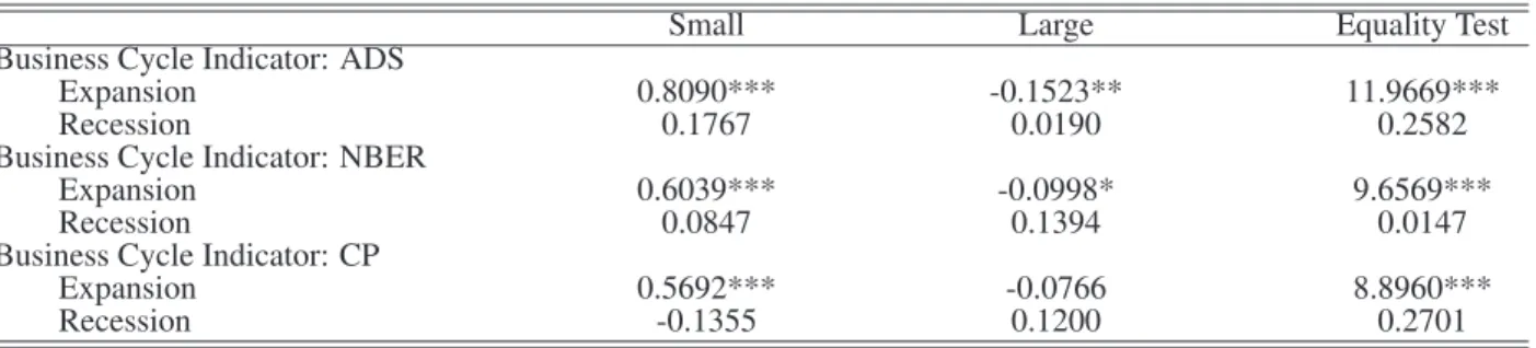
(15) econometric model as measured by the relative root mean square forecast error of 0.76.22 To analyze the robustness of our results to using alternative definitions of economic conditions, we use two additional measures of economic conditions, namely recession dummy variables based on NBER business cycle dates (NBER) and real-time recession probability of Chauvet and Piger (2008) (CP).23 The dummy variable based on NBER business cycle dates is one if the NBER defines that month to be a recession period and zero otherwise. The dummy variable based real-time recession probability is one if the probability of a recession is greater than 0.5 and zero otherwise.24 Both of these alternative definitions of economic conditions are only available at the monthly rather than the daily frequency. Hence, we assume that they remain constant within a given month. The daily correlations between these alternative measures and that based on ADS are both 0.45 for the period between 1967 and 2009 whereas the correlation between these two alternative measures is 0.84 for the same period. Table 5 presents the reactions of the first and tenth decile of size- and BM-sorted portfolios to employment news based on the econometric model in Equation (5). We estimate the empirical specification in Equation (4) only for the first and tenth decile portfolios rather than all ten portfolios. Although we present results only for the reaction to employment news, we still control for the reactions of stock returns to all the other macroeconomic news.25 The coefficient estimates are obtained via GMM with HAC standard errors rather than SUR. [INSERT TABLE 5 HERE] The reactions of small and value firms continue to be significantly different from that of large and growth firms in expansions but not in recessions. The evidence of a significant reaction to employment news in expansions is more pronounced in the later sample between 1985 and 2009. There is also some marginally significant evidence of a positive reaction of small and value firms. Overall, these results suggest that the significant difference in the reactions of small-value firms and large-growth firms to employment news is robust to using alternative definitions of the news variable and the recession periods as well as different subsamples. Finally, we analyze the robustness of our results to using alternative definitions of portfolios. Rather than analyzing the size and BM-sorted portfolios separately, we estimate the reactions of daily returns on 22. Further details on the news variable based on the econometric model is available from the author upon request. These variables are available to us from the websites of NBER and Jeremy Piger at University of Oregon. 24 This variable is only available starting February 1967. 25 We exclude the announcement day dummy variables for Unemployment Rate, Hourly Earnings, Personal Consumption Expenditures, Export Price Index, Core PPI and CPI when estimating the empirical specification for the subsample period between 1985 and 2009. These variables have the same announcement days as some other variables in the data set when we split our sample into expansions and recessions. This causes a multicollinearity problem similar to the one for Equation (3). 23. 13.

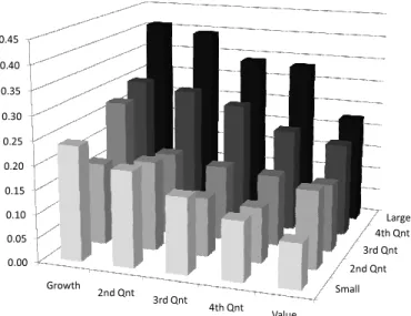
(16) the 25 size and BM cross-sorted portfolios to employment news over the business cycle. To this extent, we estimate the reaction of daily returns to employment news only on announcement days for this variable without controlling for the reaction to other macroeconomic news released on the same day.26 Here, we use the news variables defined based on the consensus median forecast from the MMS survey data and the business cycle dummy variable based on the ADS index. The sample consists of announcement days for employment numbers between February 1985 and December 2009. Figure 1 presents our empirical results. We multiply the coefficient estimates by -1 for ease of exposition. In other words, a positive number represents a negative coefficient estimate and vice versa. Our results are quite similar to those based on the ten size- or BM-sorted portfolios. There is a clear pattern for the reactions of 25 cross-sorted portfolios. The reactions of large-growth firms to employment news in expansions are larger in absolute value than those of small-value firms. There is no such clear pattern in recessions. Although not presented, the reactions in expansions are mostly significant for all portfolios whereas they are mostly insignificant in recessions. The results are similar for the news variable based on the econometric model and alternative definitions of the business cycle dummy variable. [INSERT FIGURE 1 HERE]. 4.2. Control Variables. In addition to observed macroeconomic news, stock returns might also be reacting to unobserved macroeconomic factors. Hence, ignoring the effect of these unobserved factors might affect the reaction of stock returns to observed macroeconomic news. In this section, we analyze the robustness of our results to including unobserved macroeconomic factors in our empirical specification. Specifically, we estimate the empirical specification in Equation (4) for the first and tenth decile portfolios with proxies for unobserved macroeconomic factors as control variables in addition to the observed macroeconomic news. To proxy for daily changes in unobserved macroeconomic factors, we extract principal components from several daily variables that might reflect changes in investors’ expectations about macroeconomic conditions. Our approach of extracting principal components can be considered as a special case of Andreou, Ghysels, and Kourtellos (2010) where they argue that principal components extracted form a large number of daily financial variables might help predict macroeconomic variables such as output and inflation. Specifically, we extract the first four principal components from daily changes in the 10 year treasury bond 26. rec This specification is similar to the one in (4). Specifically, we estimate the following linear specification: ri,t = β0,i 1rec,t + exp rec − 1rec,t ) + β1,i St 1rec,t + β1,i St (1 − 1rec,t ) + εi,t where St is the employment news and 1rec,t is a business cycle dummy variable.. exp β0,i (1. 14.

(17) yield, the term spread defined as the difference between the 10 year treasury bond yield and the 3 month treasury bill yield, the WTI oil price, the Commodity Research Bureau (CRB) commodity price index, the effective US exchange rate against major currencies and the ADS index. All these variables except the ADS index are available at daily frequency from Datastream. We choose to focus on the later subsample between 1985 and 2009 as some of these daily variables are not available for the whole period of the earlier sample between 1965 and 1985. The first four principal components explain 82% of the variation in these six daily variables. Our results for the reaction of stock returns to employment news do not change qualitatively when we include unobserved macroeconomic factors in our empirical specification. Although we choose not to present the results here for the sake of brevity, we briefly discuss our findings. First of all, unobserved macroeconomic factors seem to have a significant effect on daily stock returns although the effect changes with respect to the factor and the portfolio considered. More importantly, the reactions of small and value firms to employment news continue to be significantly different from those of large and growth firms in expansions. Finally, there is also some evidence that the reactions of small and large firms are different in recessions even though neither small nor large firms react significantly to employment news in recessions.. 4.3. Multivariate GARCH Specification. Daily returns are known to have time-varying conditional volatility. We have not considered this possibility in our main results in Section 3 due to the difficulty involved in estimating a multivariate model with timevarying conditional variance-covariance matrix for a large number of portfolios. However, a bivariate model for the first and tenth decile portfolios with time-varying conditional variance-covariance matrix can be estimated in a relatively straightforward manner. In this section, we analyze the reactions of stock returns to employment news in a bivariate GARCH framework. Specifically, we estimate the following diagonal VECH with the mean vector and the conditional covariance matrix of the following form: .  r1,t.   = β0rec · 1rec,t + β0exp · (1 − 1rec,t ) r10,t + β1rec · S2,t · 1rec,t + β1exp · S2,t · (1 − 1rec,t ) + β2rec · I2,t · 1rec,t + β1exp · I2,t · (1 − 1rec,t ) + εt Ht = Ω0 + Ω1 · εt−1 ε0t−1 + Ω2 · Ht−1. 15. (6).

(18) where β0rec , β0exp , β1rec , β1exp , β2rec and β2exp are two-by-one vectors of coefficients and “·” is the elementby-element product. S2,t and I2,t are two-by-one vectors of employment news and the corresponding announcement days, respectively, and εt is the two-by-one vector of error terms with the conditional covariance of Ht . The coefficient matrices in the conditional variance equation (Ω0 , Ω1 , Ω2 ) are indefinite two-by-two symmetric matrices. We estimate the bivariate GARCH specification via maximum likelihood with Bollerslev-Wooldridge robust standard errors. Our results for the reaction of stock returns to employment news do not change qualitatively when we control for time-varying conditional heteroskedasticity of daily returns.27 Although we choose not to present the results here for the sake of brevity, we briefly discuss our findings. First of all, not surprisingly, daily stock returns exhibit time-varying conditional volatility as suggested by the significant coefficient estimates of the elements of Ω1 and Ω2 . More importantly, the reactions of small and value firms to employment news continue to be significantly different from those of large and growth firms in expansions. Finally, there is also some evidence that small stocks react positively to employment news in recessions suggesting that good news about improving labor market conditions is actually good news for small stocks in recessions.. 5. Fundamentals and Macroeconomic News. Our empirical results suggest that the reactions of returns on large-growth firms to employment news in expansions are significantly different from those of small-value firms. In this section, we analyze whether differences in the reactions of fundamentals can account for the differences in the observed reactions of size- and BM-sorted portfolios to employment news. To this extent, we first establish that small-value firms continue to react to employment news differently from large-growth firms at the monthly frequency. Using the Campbell and Shiller return decomposition approach, we then decompose returns into cash flow and discount rate components and analyze the effect of employment news on these two components over the business cycle at the monthly frequency.. 5.1. The Return Decomposition Approach. We first briefly discuss the return decomposition approach and related issues in the empirical implementation of this approach. To decompose the returns into fundamentals, we use the return decomposition approach 27 We also considered including the news variable and the announcement day dummy variable in the variance equation. Our results on the reaction of stock returns to employment news do not change qualitatively. There is some marginally significant evidence that the conditional volatility of stock returns reacts to employment news.. 16.

(19) discussed in Campbell and Shiller (1988a), Campbell and Shiller (1988b), and Campbell (1991).28 For completeness, we briefly discuss the theoretical background for the return decomposition before focusing on the details of the empirical implementation.29 Campbell and Shiller (1988a) show that the excess return on a stock can be approximated as a linear combination of revisions in expected future dividends and expected future returns as follows: ηi,t ≡. ∗ ri,t. −. ∗ Et−1 [ri,t ]. ¸ ·X ¸¶ µ ·X ∞ ∞ j j ρi ∆di,t+j = Et ρi ∆di,t+j − Et−1 j=0. j=0. µ ·X ¸ ·X ¸¶ ∞ ∞ j ∗ j ∗ − Et ρi ri,t+j − Et−1 ρi ri,t+j j=1. j=1. ≡ ηi,d,t − ηi,r,t. (7). ∗ is the excess return on the ith portfolio in period t, ∆d is the one period change in log dividends where ri,t i,t. (or equivalently the dividend growth rate) and Et [·] denotes the expectation operator given the information set in period t. ρi is a parameter of linearization and is defined as ρi ≡ 1/(1 + exp(di − pi )) where pi is the log price of the ith portfolio and (di − pi ) is the average log dividend-price ratio. Campbell and Vuolteenaho (2004a) note that ρi is a discount coefficient that can be related to either the average log price dividend ratio or the average consumption wealth ratio. ηi,t is the unexpected excess return, ηi,d,t is the change in the expectations of future cash flows and ηi,r,t is the change in the future rates used by investors to discount the cash flows (or equivalently, the change in the equity premiums or the future excess returns). Empirically, one can employ a forecasting model to obtain proxies for the relevant expectations in the log-linear approximation.30 Following the previous literature, we model the dynamics of the returns on 28 The Campbell and Shiller return decomposition approach is widely used in the empirical finance literature. A partial list of studies using the Campbell and Shiller decomposition for various purposes include Campbell and Ammer (1993), Campbell and Mei (1993), Patelis (1997), Vuolteenaho (2002), Campbell and Vuolteenaho (2004a), Campbell and Vuolteenaho (2004b), Bernanke and Kuttner (2005), Hecht and Vuolteenaho (2006) and Campbell, Polk, and Vuolteenaho (2010). 29 The reader is referred to Campbell (1991) and Campbell and Shiller (1988a) for further details. 30 One can also use long horizon regressions instead of a VAR as in Cohen, Polk, and Vuolteenaho (2003) to decompose the returns. They argue that long horizon regression is a more appropriate approach for managed portfolios and estimating a VAR for the size- or BM-sorted portfolios might be problematic. The key assumption underlying the VAR approach is that this period’s dependent variables are next period’s independent variables. This assumption might be violated for portfolios with managed weights such as the Fama-French size- or BM-sorted portfolios as they are rebalanced June of each year according to changes in market capitalizations and BM ratios. For example, the VAR approach might incorrectly link the dependent variables for small firms to independent variables for large firms. This is especially problematic when one uses annual data to estimate the VAR as in Cohen, Polk, and Vuolteenaho (2003). However, the violation of this assumption is less of a problem for monthly data. Furthermore, Boudoukh, Richardson, and Whitelaw (2008) argue that the long horizon predictability of stock returns might be spurious. Hence, we opt to choose the simpler and more elegant alternative of VAR.. 17.

(20) portfolios as components of the following VAR(1) model:  zi,t ≡ .  ∗ ri,t. xi,t.  = Ai zi,t−1 + ξi,t. (8). where zi,t is a ((k + 1) × 1) vector process whose first element is the excess return on the ith portfolio in ∗ and ξ ((k + 1) × 1) month t. xi,t is a (k × 1) vector process whose elements have forecasting power for ri,t i,t. is the vector of the unpredictable components of the elements in the VAR. Using the VAR model in Equation (8) and the log-linearization in Equation (7), one can obtain estimates of the unexpected excess returns (ηi,t ), the cash flow component (ηi,d,t ), and the discount rate component (ηi,r,t ). Specifically, let “ˆ” denote the estimated values, e.g. ξî,t denotes the residuals (or equivalently, the one-period forecast errors) from the VAR estimation, then ηî,t , ηî,r,t and ηî,d,t can be expressed as follows: ηî,t = e01 ξî,t ∞ X 0 ˆ i )−1 ξî,t ˆ i (I − ρî A ˆ j ξî,t = e0 ρî A ηî,r,t = e1 ρˆji A 1 i. (9). j=1 ∗ î (I − ρî A ˆ i )−1 )ξî,t ˆt−1 [r∗ ]) + ηî,r,t = e0 (I + ρî A ηî,d,t = (ri,t −E i,t 1. (10). where I is the (k + 1) × (k + 1) identity matrix and e1 ((k + 1) × 1)) is the first unit vector, i.e. a vector whose first element is one and the others are zero. In the empirical implementation of the Campbell and Shiller approach, one needs to choose state variables that have forecasting power for returns. However, one needs to be careful about what state variables to include in the VAR specification as the results tend to be sensitive to the choice of state variables. In a recent paper, Chen and Zhao (2009) demonstrate the sensitivity of the return decomposition approach to the state variables used in the empirical specification. They emphasize that the impact of a state variable on the decomposition is a function of its persistence. They identify the 10-year smoothed price-earnings ratio with an autocorrelation of 0.99 to be the variable that has the greatest impact on the results of the decomposition in their study. They also suggest several possible remedies. In this paper, we use one of the suggested remedies, namely the principal components approach, to minimize the effect of the choice of state variables on our results. Specifically, we include the first eight principal components from a large set of predictor variables including the value spread used in Campbell and Vuolteenaho (2004a) and almost all variables used in Welch and Goyal (2008).31 In addition to these eight principal components, we also 31 Our data set includes dividend payout ratio, stock variance, default return spread, long term yield, long term return, inflation, term spread, treasury bill rate, default yield spread, dividend price ratio, dividend yield, earning price ratio, book to market ratio,. 18.

(21) include returns on the five Fama-French industry portfolios as state variables in our VAR specification since there is some empirical evidence that the industry portfolios have some predictive power for returns on sizeand BM-sorted portfolios (see Kong, Rapach, Strauss, Tu, and Zhou (2009)).. 5.2. The Reaction of Unexpected Excess Monthly Returns to Employment News. In this section, we analyze the reactions of unexpected returns to employment news at the monthly frequency. To this extent, we choose to use employment news based on the econometric model in Equation (5) rather than news variable based on survey expectations. The news variable based on the econometric model is more appropriate for an analysis at monthly frequency. First of all, the news variable based on the econometric model allows us to use a longer sample period starting in 1965. A longer sample is especially important at the monthly frequency where the number of observations is rather limited. Secondly, the news variable based on the econometric model uses information available up to the last day of the previous month whereas the news variable based on survey expectations might contain information related to the current month. This distinction is important for an analysis at monthly frequency since survey participants might incorporate additional information into their expectations and one might not observe a significant reaction of stock returns to employment news at the monthly frequency. To analyze the reaction of unexpected excess monthly stock returns to employment news, we estimate the following empirical specification via GMM with HAC standard errors: exp exp rec rec ηî,t = β0,i 1rec,t + β0,i (1 − 1rec,t ) + β1,i S2,t 1rec,t + β1,i S2,t (1 − 1rec,t ). + β2,i,DR ηˆmkt,r,t + β2,i,CF ηˆmkt,d,t + εi,t. (11). where ηî,t is the unexpected excess return on portfolio i in month t, ηˆmkt,r,t and ηˆmkt,d,t are the cash flow and discount rate components of the market portfolio (CRSP value-weighted index). S2,t is the employment news in month t and 1rec,t is the recession dummy variable. Our empirical model is motivated by the two-beta model of Campbell and Vuolteenaho (2004a) and Campbell, Polk, and Vuolteenaho (2010). This empirical specification allows us to analyze the reaction of unexpected monthly returns to employment news while controlling for other changes in the fundamentals of the aggregate market portfolio. Table 6 presents the reaction of unexpected monthly returns to employment news . 10-year smoothed earning price ratio, net equity expansion and value spread. We did not have access to several other variables such as the book-to-market spread, percent equity issuing, net equity expansion and consumption-wealth-income ratio used either in Welch and Goyal (2008) or Chen and Zhao (2009). We refer the reader to Welch and Goyal (2008) or Chen and Zhao (2009) for detailed variable definitions.. 19.

(22) [INSERT TABLE 6 HERE] Monthly returns on large and growth firms continue to react negatively to higher than expected employment numbers in expansions and the reactions of large and growth firms continue to be insignificant during recessions. On the other hand, monthly returns on small and value firms react positively to positive employment news and the reactions of small and value firms remain insignificant in recessions.32 More importantly, the reactions of large and growth firms at monthly frequency continue to be significantly different from those of small and value firms in expansions but not in recessions, similar to their initial daily reactions.. 5.3. Reaction of Fundamentals to Employment News. We now focus on the reaction of cash flow and discount rate components to employment news over the business cycle. To this extent, we estimate the empirical specification in Equation (11) via GMM with HAC standard errors where we replace the dependent variable with the cash flow or the discount rate components of size- and BM-sorted portfolios. Table 7 presents our empirical results. [INSERT TABLE 7 HERE] We start with the reactions of cash flows and discount rates of size-sorted portfolios. First of all, employment news has a positive and significant effect on the discount rate for large firms in expansions but not in recessions. This result suggests that the rate used by investors to discount the cash flows from large firms increases (decreases) significantly following higher (lower) than expected employment numbers in expansions. On the other hand, the reaction of the discount rate for small firms is insignificant in both expansions and recessions suggesting that the investors do not change their discount rate for small firms following employment news. Although employment news reveals important information about the discount rate for large but not small firms, the effect of employment news on the discount rates for small and large firms is not statistically distinguishable. When we compare the effect of employment news on the cash flows of size-sorted portfolios, we find that the reactions of cash flows are statistically different from each other 32 The slight discrepancy between the daily and monthly reactions of small and value firms is mainly due to the earlier part of our sample period between 1965 and and 1985. First of all, in an unreported analysis, we find that the reactions of both daily and monthly returns on small and value firms to employment news are significant and positive for the earlier subsample period between 1965 and 1985 but statistically insignificant for the later subsample period between 1985 and 2008. Secondly, the discrepancy between the daily and monthly results for small and value firms might also be due to possible delayed reactions of daily returns on these portfolio. Once again, we find some empirical evidence in support of delayed reactions of daily returns on small and value firms only in the earlier subsample. Specifically, two-day returns on small and value firms following employment announcements react significantly to employment news only in the earlier subsample but not in the later subsample. However, even in the earlier sample, two-day returns on small-value and large-growth firms following employment announcements continue to react significantly different from each other.. 20.

(23) in expansions. Employment news has a significant positive effect on the cash flows of small firms in expansions whereas the effect is insignificant on the cash flows of large firms in both expansions and recessions. These results suggest that the significant difference in the reactions of size-sorted portfolios to employment news in expansions is mainly due to the significant difference in the reactions of their cash flows although there is evidence that the discount rate of large firms is also sensitive to employment news in expansions. We now turn our attention to the reactions of cash flows and discount rates of BM-sorted portfolios. First of all, there is no statistically significant evidence that employment news has an effect on the discount rates of BM-sorted portfolios. On the other hand, the reactions of cash flows of BM-sorted portfolios are significantly different from each other in expansions. This significant difference is mainly due to a positive and significant reaction of cash flows of value firms to employment news in expansions. These results suggest that the significant difference in the reactions of BM-sorted portfolios to employment news in expansions is mainly due to the significant difference in the reactions of their cash flows. The Campbell and Shiller approach directly models the discount rate without having to model the dynamics of the cash flows. In other words, the cash flows in the Campbell and Shiller approach are treated as residuals that are not captured by the predictive relation between state variables and returns. Hence, the success of the Campbell and Shiller approach in decomposing the returns into cash flow and discount rate components depends on the predictive power of the state variables for returns on different portfolios. As discussed in Chen and Zhao (2009), different state variables have different predictive powers for returns and the results are sensitive to what state variables are used. Although we included a large number of predictor variables to decrease the sensitivity of our results to choice variables33 , one might still argue that the predictability of returns differs across portfolios even if the same variables are used. To this extent, we analyze the reaction of cash flows to changes in labor market conditions by a “model-free” approach similar to the one used in Boyd, Hu, and Jagannathan (2005). Before discussing the approach and our results, we would like to note several facts about the predictability of different portfolios. Although there are some differences in the predictability of different portfolios (the in-sample R2 for small, large, growth and value firms are 12%, 8%, 8% and 9%, respectively), these differences are neither statistically nor economically significant. Secondly, these differences cannot explain the observed differences in the reactions of cash flows. The cash flows of small and value firms react stronger than those of large and growth firms. However, the predictabil33. We also analyzed the robustness of our results to many other factors. We changed the number of principal components used as state variables. Our results do not change significantly when we include only the first five principal components as in Chen and Zhao (2009). We excluded the returns on industry portfolios and the 10-year smoothed earnings price ratio, the variable identified by Chen and Zhao (2009) to have the most significant effect on the results of the Campbell and Shiller decomposition. We find that our results do not change significantly whether we choose to include or exclude these variables from our data set. We also use different reasonable values for the parameter of linearization, ρi , which does not seem to have a significant effect on our results.. 21.

(24) ity of small and value firms, as measured by their R2 , is also larger than that of large and growth firms. If anything, the higher predictability of small and value firms should bias downward the reaction of cash flows of these firms since cash flows are treated as residuals in the Campbell and Shiller decomposition. Our “model-free” approach analyzes the true relation between dividend growth rates and actual rather than unexpected changes in the employment numbers. As in Boyd, Hu, and Jagannathan (2005), the intuition underlying this approach is that investors are good econometricians who analyze market data and make forecasts. Specifically, we estimate the following empirical specification via GMM with HAC standard errors: exp rec ∆di,t+s = β0,i,s + β1,i,s ∆EM Pt 1rec,t + β1,i,s ∆EM Pt (1 − 1rec,t ) + εi,t+s. for s = 1, 2, 3, 4, 5, 6 (12). where ∆di,t+s is the monthly log dividend growth and ∆EM Pt is the actual change in real-time employment numbers. The portfolio dividends are calculated using monthly returns with and without dividends as x in Bansal, Dittmar, and Lundblad (2005). Briefly, let ri,t+1 and ri,t+1 denote monthly return on portfolio. i with and without dividends, respectively. Then, the dividend paid out by portfolio i can be calculated as x x Di,t+1 = (ri,t+1 − ri,t+1 )Pi,t where Pi,t denotes the price level of portfolio i with Pi,t+1 = (1 + ri,t+1 )Pi,t. and Pi,0 = 1. Dividends are known to exhibit seasonal patterns due to dividend smoothing and corporate policies. To this extent, we calculate the log dividend growth as the log change in the trailing twelve months moving average dividends. [INSERT TABLE 8 HERE] Table 8 presents our results. On average, there is a positive and significant relation between dividend growth rates of size-sorted portfolios and changes in employment numbers in expansions but not in recessions. More importantly, the effects of changes in employment numbers on the dividend growth rates of small and large firms in expansions are significantly different from each other up to four months. On the other hand, there is a strong positive relation between dividend growth rates of value firms and changes in employment numbers in both expansions and recessions. There is no such significant relation between the dividend growth rates of growth firms and changes in employment numbers. However, the difference is significant only at a six month horizon. These results provide additional support for our findings on the sensitivities of cash flows of portfolios with different characteristics based on the Campbell and Shiller decomposition. Specifically, we confirm in a “model-free” framework that the cash flows of small and value firms are more sensitive to changes in labor market conditions than those of large and growth firms.. 22.

(25) 6. Discussion and the Related Literature. As discussed in the introduction, our results are related to two strands of the literature. First is the literature on the reactions of high-frequency stock returns to macroeconomic news. Pearce and Roley (1985) are among the first to analyze the reaction of daily returns on an aggregate index to macroeconomic news. They find that news about many macroeconomic variables have no significant effect on stock prices. McQueen and Roley (1993) argue that the insignificant reaction of stock returns to macroeconomic news might be due to the time-varying effect of macroeconomic news on stock returns over the business cycle. Specifically, they analyze the reaction of daily returns on the S&P 500 index to macroeconomic news over the business cycle. They find that the stock market reacts negatively to news about higher than expected real economic activity in expansions and argue that this negative relation is due to the larger increase in discount rates relative to expected cash flows. Boyd, Hu, and Jagannathan (2005) provide a similar explanation for the negative reaction of S&P 500 returns to employment news in expansions. Our results are in line with the findings of these two studies if one considers that the S&P 500 index is a proxy for large firms.34 In line with the results of McQueen and Roley (1993) and Boyd, Hu, and Jagannathan (2005), we also find that large firms react negatively to higher than expected employment numbers in expansions but not in recessions. Our results based on the Campbell and Shiller decomposition suggest that the negative reaction of large firms to higher than expected employment numbers is mainly due to an increase in the discount rate used by investors following positive employment news in expansions. Our results for other macroeconomic variables are also broadly consistent with those in McQueen and Roley (1993), Flannery and Protopapadakis (2002) and Andersen, Bollerslev, Diebold, and Vega (2007). Second is the literature on the low-frequency relation between returns, fundamentals and aggregate conditions. We group this strand of the literature into three categories and discuss our results in relation to these three categories separately. Fama and French (1995) are among the first to study the link between returns on size- and BM-sorted portfolios and the behavior of their economic fundamentals. They argue that value firms earn higher average returns than growth firms since they have persistently lower earnings and higher financial leverage (signaling higher risk of financial distress) than growth firms. Several papers, including Berk, Green, and Naik (1999), Gomes, Kogan, and Zhang (2003), Carlson, Fisher, and Giammarino (2004), Zhang (2005) and Cooper (2006), develop theoretical frameworks to link firm characteristics and expected returns to economic fundamentals. For example, Zhang (2005) argues that assets-in-place of value firms are riskier than growth options especially during bad times when the price of risk is high. He develops a model 34. The daily and monthly correlations between returns on the tenth decile of the ten size-sorted portfolios and the S&P 500 index are both 99% for the sample period between 1965 and 2009.. 23.