Araar: Département d’économique and CIRPÉE, Université Laval, Canada
aabd@ecn.ulaval.ca
Duclos: Département d’économique and CIRPÉE, Université Laval, Canada
jyves@ecn.ulaval.ca
Audet: GRÉDI, Université de Sherbrooke, Canada
maudet@worldbank.org
Makdissi: Département d’économique, CIRPÉE and GRÉDI, Université de Sherbrooke, Canada
paul.makdissi@ecn.USherbrooke.ca
We are grateful to Dr. Lourdes Trevio and Professor Jorge Valero Gil for their invitation to present this paper at the Eight Symposium on “Capital Humano, Crecimiento, Probreza: Problemática Mexicana” that took place in Monterrey, Mexico on Cahier de recherche/Working Paper 07-09
Testing for Pro-Poorness of Growth, with an Application to Mexico
Abdelkrim Araar Jean-Yves Duclos Mathieu Audet Paul Makdissi
Abstract:
This paper proposes techniques to test for whether growth has been pro-poor. We first review different definitions of pro-poorness and argue for the use of methods that can generate results that are robust over classes of pro-poor measures and ranges of poverty lines. We then provide statistical procedures that rely on the use of sample data to infer whether growth has been pro-poor in a population. We apply these procedures to Mexican household surveys for the years of 1992, 1998 and 2004. We find strong statistical evidence that Mexican growth has been absolutely anti-poor between 1992 and 1998, absolutely pro-poor between 1998 and 2004 and between 1992 and 2004, and relatively pro-poor between 1992 and 2004 and between 1998 and 2004. The relative assessment of the period between 1992 and 1998 is statistically too weak to lead to a robust evaluation of that period.
Keywords: Pro-poor growth, poverty, inequality
1 Introduction
It would seem uncontroversial to think of the concept of the pro-poorness of growth as concerning the impact of growth on the wellbeing of the poor. Like many other distributive concepts, however, its precise meaning and its usefulness
are essentially a matter of judgement1. There are at least three areas of contention
in trying to make the assessment of pro-poorness operational. The first fundamen-tal issue is whether the concept of pro-poorness should be absolute or relative. A second issue is what poverty line should be chosen to separate the poor from the non-poor. A final issue is how we should assess in the aggregate the heterogeneous impact of growth in a population that is also heterogeneous.
This paper attempts to address all these three issues. It also proposes proce-dures to make it statistically and empirically feasible to test for the pro-poorness of distributive changes. To do this, we first rely on the definitional framework of Duclos and Wodon (2004). Roughly speaking, and according to that framework, a relative definition of pro-poorness judges a distributive change to be pro-poor if the proportional change in the incomes of the poor is no less than some norm, often set as the growth rate in mean income or in some quantile such as median income. For an absolute definition, the incomes of the poor need to grow by an absolute amount that is no less than some norm, this time often set as zero or as some proportion of the absolute change in mean or median incomes. These dif-ferent definitions can also be linked to the usual concepts of absolute and relative poverty. With relative poverty, the poverty line is usually defined as a proportion of some central tendency of an income distribution; with absolute poverty, the real level of the poverty line normally remains the same even if the income distribution changes.
The framework of Duclos and Wodon (2004) also enables to get around the difficulty of having to choose 1) a poverty line to separate the poor from the non-poor, and 2) a set of normative weights to differentiate among the poor. The framework does this by investigating how ppoor judgements can be made ro-bust to wide classes of pro-poor evaluation functions and to ranges of poverty
lines.2
1See, among many recent contributions to that debate, Bourguignon (2003), Bruno, Ravallion,
and Squire (1999), Dollar and Kraay (2002), Eastwood and Lipton (2001), United-Nations (2000), and World-Bank (2000).
2Many different approaches have been proposed to separate the poor from the non-poor and to
compute and aggregate index of pro-poorness. See, for instance, McCulloch and Baulch (1999), Kakwani, Khandker, and Son (2003), Kakwani and Pernia (2000), Ravallion and Chen (2003),
In practice, household data surveys are of course needed to check if growth is pro-poor or not. This leads us to consider issues of estimation, sampling variabil-ity and statistical inference. We first propose sets of null and alternative hypothe-ses for testing for absolute and relative pro-poorness of growth. We then define various estimators of the statistics of interest and derive their sampling distribu-tion, taking full account of the complexity of the usual forms of sampling design. This enables us inter alia to draw confidence intervals around the differences that must be signed in order to conclude that a change has been robustly pro-poor — or not. To our knowledge, this is the first paper to address the issue of pro-poor comparisons within a rigorous statistical setting.
We then illustrate the usefulness of these techniques by applying them to Mex-ico’s National Income and Expenditure Surveys collected in 1992, 1998 and 2004. Two main conclusions emerge. First, we find strong normative and statistical evi-dence that Mexican growth has been absolutely anti-poor between 1992 and 1998, absolutely pro-poor between 1998 and 2004 and between 1992 and 2004, and rel-atively pro-poor between 1992 and 2004 and between 1998 and 2004. This is useful and robust evidence on Mexico’s distributional change during a period of significant economic turbulences and transformations.
Second, we see how and why observing pro-poorness in samples does not imply that we can immediately infer it for populations of interest. For instance, although the sample estimates might naively suggest that the distributive change within the period between 1992 and 1998 is first-order relatively pro-poor, the use of our statistical inference techniques indicates that the evidence is statistically too weak to lead to a robust relative pro-poor evaluation of that period. We also see that, contrary to what measurement theory usually implies for poverty dom-inance relationships, moving to higher orders does not necessarily lead to more definite comparisons. For instance, statistical uncertainty in comparing 1992 to 1998 is amplified when moving from first-order to second-order relative compar-isons, which also means that second-order relative comparisons are statistically less strong than first-order ones.
The rest of the paper is as follows. Section 2 presents the measurement frame-work. Section 3 deals with issues of estimation and statistical inference. Section 4 applies the measurement and statistical techniques to Mexican data. Section 5 concludes.
2 Measurement framework
2.1 The setting
Let y1 =¡y1 1, y12, · · · , y1n1 ¢ ∈ <n1+ be a vector of non-negative initial incomes3
(at time 1) of size n1, and let y2 =
¡ y2
1, y22, · · · , yn22 ¢
be an analogous vector of
posterior incomes (at time 2) of size n2.
The following draws extensively from Duclos and Wodon (2004). To
deter-mine whether the movement from y1 to y2 is pro-poor, we first need to define a
standard with which this assessment can be made. First consider the case of a rel-ative standard, which we will take in this paper as the growth in average incomes, denoted by g. Intuitively, for growth to be relatively pro-poor, we wish the poor’s “representative” income to undergo a proportional change that is no less than g. That growth g can be negative as well as positive. Relative pro-poorness is con-sistent, for instance, with the view of Kakwani and Pernia (2000) that “promoting pro-poor growth requires a strategy that is deliberately biased in favor of the poor so that the poor benefit proportionately more than the rich. (p.3)”.
Then denote by z > 0 a poverty line, defined in real terms. Let W (y1, y2, g, z)
be the pro-poor evaluation function that we want to use. It is defined as the
differ-ence between two evaluation functions Π (y1, z) and Π∗(y
2, g, z), each for time 1
and time 2, respectively, and which are analogous to poverty indices for each of the two time periods:
W (y1, y2, g, z) ≡ Π∗(y
2, g, z) − Π (y1, z) . (1)
The change from y1to y2will be deemed pro-poor if W (y1, y2, g, z) ≤ 0.
Clearly, whether the distributional change will be deemed pro-poor will
de-pend on the way in which z, Π, and Π∗ will be chosen. To put some structure on
the form of W in which we should be interested, we need to invoke a few axioms. The first one is a focus axiom: W is not sensitive to marginal changes in values of
y1 that exceed z. The distribution of min(yi, z) is thus sufficient for judgements
of pro-poorness.
Second, we can postulate an axiom of population invariance. This says that adding a replication of a population to that same population has no impact on W . It is a common axiom in welfare economics that enables us to make pro-poor judgements even when the absolute population size varies across the distributions.
A third axiom is that of anonymity: this says permuting the incomes of any two persons in any given distribution should not affect pro-poor judgements. Note that this axiom will typically lead to violations of the well-known Pareto efficiency-criterion; our framework does not require that none of the poor be penalized by a distributional change for that change to be declared pro-poor. Were we not to impose this axiom, it would be practically impossible to order the initial and posterior distributions in the presence of a large number of individuals, and we would also need panel data.
The next axiom is a normalization one: if there has been no distributional change, and thus also no change in mean income, then W = 0.
We may then also impose an axiom of monotonicity: for a given g, if anyone’s posterior income increases, W should not increase, and may sometimes fall. In-creasing posterior incomes make it more likely that the distributive change will be declared pro-poor.
2.2 Relative pro-poor judgements
We can then also axiomatize our view of relative pro-poorness. Formally, suppose that y/ (1 + g) = ˙y/ (1 + ˙g). Then, according to relative judgements of pro-poorness, y and ˙y should be judged equally pro-poor by W (using standard g
and ˙g respectively) regardless of the initial distribution y1.
Combined together, the axioms that we have invoked until now define what we can term to be a first-order class of relative pro-poor evaluation functions.
Denote that class as Ω1(g, z+). Formally, the class Ω1(g, z+) regroups all of the
functions W that satisfy the focus, the population invariance, the anonymity, the
monotonicity, the normalization and the relative axioms, and for which z ≤ z+.
Now let Fj(y) be the distribution function of distribution j. Also define as
Qj(p) the quantile function for distribution Fj. This is formally defined as Qj(p) =
inf{s ≥ 0|Fj(s) ≥ p} for p ∈ [0, 1]. With a continuous distribution and a strictly
positive income density, Q(p) is simply the inverse of the distribution function, and it is the income of that individual who is at rank p in the distribution.
The popular class of FGT indices is then given by:
Pj(z; α) =
Z Fj(z)
0
(1 − Qj(p)/z)αdp. (2)
Pj(z; α = 0) is the headcount index (and the distribution function) at z, and
a movement from y1 to y2 will be judged pro-poor by all pro-poor evaluation
functions W (·, ·, g, z) that are members of Ω1(g, z+) if and only if
P2((1 + g)z; α = 0) ≤ P1(z; α = 0) for all z ∈ [0, z+]. (3)
A distributional change that satisfies (3) is called first-order relatively
pro-poor since all pro-pro-poor evaluation functions within Ω1(g, z+) will find that it is
pro-poor, and this, for any choice of poverty line within [0, z+] and any W that
obeys the above-defined axioms. Verifying (3) simply involves checking whether
— over the range of poverty lines [0, z+] — the headcount index in the initial
distribution is larger than the headcount index in the posterior distribution when that distribution is normalized by 1 + g.
An alternative and equivalent way of checking whether a distributional change can be declared first-order relatively pro-poor is to compare the ratio of the quan-tiles to (1 + g), or, if g is growth in mean income, to compare the growth in quantiles to the growth in the mean. That this, we check whether, for all p ∈
[0, F1(z+)], Q2(p) Q1(p) ≥ 1 + g (4) or whether Q2(p) − Q1(p) Q1(p) ≥ g. (5)
Using (5) is equivalent to Ravallion and Chen (2003)’s suggestion to use “growth incidence curves” to check whether growth is pro-poor. These curves show the growth rates of living standards at different ranks in the population.
First-order pro-poor judgements can be demanding in expansion periods. They require all quantiles of the poor to undergo a rate of growth at least as large as the rate of growth in mean income. We may, however, be willing to relax this con-dition if the rate of growth for the poorer among the poor is sufficiently large to exceed g even though the rate of growth for the not-so-poor may be below g. An axiom that captures this is the distribution sensitivity axiom. It says that the eval-uation functions Π should give more weight to the poorer than to the not-so-poor among the poor. Distribution-sensitive pro-poor judgements imply that shifting incomes from the richer to the poorer is by itself a pro-poor distributional change. This axiom is known as the Pigou-Dalton principle in the welfare literature.
Adding the distribution-sensitive axiom to the earlier axioms defines a
is made of all functions W (·, ·, g, z) that satisfy the focus, the population invari-ance, the anonymity, the monotonicity, the normalization, the distribution
sensi-tivity and the relative axioms, and for which z ≤ z+.
It can then be shown that a movement from y1 to y2 will be judged pro-poor
by all pro-poor evaluation functions W (·, ·, g, z) that are members of Ω2(g, z+) if
and only if
P2((1 + g)z; α = 1) ≤ P1(z; α = 1) for all z ∈ [0, z+]. (6)
As for (3), a distributional change that satisfies (6) is called second-order rela-tively pro-poor since all pro-poor evaluation functions will find that it is pro-poor,
and this, for any choice of poverty line within [0, z+] and for any W that obeys the
above-mentioned axioms for Ω2(g, z+). Verifying (6) simply involves checking
whether the average poverty gap in the initial distribution is larger than that in the posterior distribution when that distribution is normalized by 1 + g and this, over
the range of poverty lines [0, z+].
As for first-order pro-poor judgements, there are alternative ways of checking condition (6). The cumulative income up to rank p (the Generalized Lorenz curve at p, see Shorrocks 1983) is given by
Cj(p) =
Z p
0
Qj(q)dq. (7)
The use of the Generalized Lorenz curve provides an intuitive sufficient condition for checking second-order relative pro-poorness. A distributional change is indeed
second-order relatively pro-poor if for all p ∈ [0, F2(z+)],
λ(p) ≡ C2(p) C1(p)
≥ 1 + g. (8)
Expression (8) involves computing the growth rates in the cumulative incomes of proportions p of the poorest, and to compare those growth rates to g. For 1 + g equal to the ratio of mean income, condition (8) is equivalent to checking whether
the Lorenz curve for y2 is above that of y1for the range of p ∈ [0, F2((1 + g)z+)].
2.3 Absolute pro-poor judgements
Absolute pro-poor judgements are made by comparing the absolute change in the poor’s incomes to some absolute pro-poor standard. Denote that standard as a.
invariant” in y and a, or that the pro-poor judgement should be neutral whenever the poor gain in absolute terms the same as the standard a. Hence, this axiom demands that if y + a = ˙y, then W (y, ˙y, a, z) = 0. This allows us to define
formally the class of first-order absolute pro-poor evaluation functions ˜Ω1(a, z+)
as made of all those functions W (·, ·, a, z) which satisfy the focus, the population, the anonymity, the monotonicity, the normalization and the absoluteness axioms,
and for which z ≤ z+. We will later set a to zero for the empirical illustration of
this paper.
We can then show that a movement from y1 to y2 will be judged first-order
absolutely pro-poor (that is, pro-poor by all evaluation functions W (·, ·, a, z) that
are members of ˜Ω1(a, z+)) if and only if
P2(z + a; α = 0) ≤ P1(z; α = 0) for all z ∈ [0, z+]. (9)
An equivalent way of checking whether a distributional change can be declared first-order absolutely pro-poor is to compare the absolute change in the values of
the quantiles for all p ∈ [0, F1(z+)]:
Q2(p) − Q1(p) ≥ a. (10)
An analogous result holds for absolute second-order pro-poor judgements. These judgements also obey the axiom of distribution sensitivity: they are made
on the basis of the class of indices ˜Ω2(a, z+), which is defined as for ˜Ω1(a, z+)
but with the additional requirement of distribution sensitivity. We can then show
that a movement from y1 to y2 will be judged second-order absolutely pro-poor
if and only if
(z + a)P2((z + a; α = 1) ≤ zP1(z; α = 1) for all z ∈ [0, z+]. (11)
A sufficient condition for condition (11) is then to verify whether, for all p ∈
[0, F2(z++ a)], the change in the average income of the bottom p proportion of
the population is larger than a:
C2(p) − C1(p) ≥ ap. (12)
3 Estimation and statistical inference
In practice, household data surveys are needed to check if growth is pro-poor or not. This forces us to deal with issues of estimation, sampling variability and statistical inference. Indeed, a difference observed in a sample may not be empir-ically strong enough to be significant from a statistical point of view.
3.1 Null and alternative hypotheses for testing pro-poorness of
growth
Each of the conditions noted in Sections 2.2 and 2.3 above takes the form
of testing whether ∆s(z) ≤ 0 or ∆s(p) ≥ 0 over some range of z or p. This
therefore involves testing jointly over a set of null hypotheses. For primal tests of pro-poorness, our formulation of our null hypothesis is thus that of a union of null hypotheses
H0 : ∆s(z) > 0 for some z ∈ [0, z+] (13)
to be tested against an alternative hypothesis which is an intersection of alternative hypotheses
H1 : ∆s(z) ≤ 0 for all z ∈ [0, z+]. (14)
For dual tests, we set a union of null hypotheses
H0 : ∆s(p) < 0 for some p ∈ [0, 1] (15)
to be tested against an intersection of alternative hypotheses
H1 : ∆s(p) ≥ 0 for all p ∈ [0, 1]. (16)
Our decision rule is to reject the union set of null hypotheses in favor of the inter-section set of alternative hypotheses only if we can reject each of the individual hypotheses in the null set at a 100·θ% significance level. This can be conveniently carried out using a 100 · (1 − θ)% one-sided confidence interval, a devise we use repeatedly in the empirical application below.
To see how this can be done, denote by ˆ∆s(z) the sample estimator of ∆s(z),
by ∆s
0(z) its sample value, and by σ2∆ˆs(z) the sampling variance of ˆ∆
s(z). Let
ζ(θ) be the (1 − θ)-quantile of the normal distribution. Given that by the law of large numbers and the central limit theorem, all of the estimators used in this paper can be shown to be consistent and asymptotically normally distributed, we
can use ∆s
0(z) ± σ∆ˆs(z)ζ(θ) as alternative lower and upper bounds for one-sided
confidence intervals for ∆s(z). For instance, an upper-bounded confidence
inter-val ∆s
0(z) + σ∆ˆs(z)ζ(θ) shows all of the values of η for which we could not reject
a null hypothesis H0 : ∆s(z) > η in favor of H1 : ∆s(z) ≤ η. Our decision rule
is then to reject the set of null hypotheses (13) in favor of (14) if:
∆s
Note that the most common procedure until now to test for such relations of “dominance” has been to posit a null hypothesis of dominance (an intersection set of hypotheses) against an alternative of non dominance (a union set of converse hypotheses) — see for instance Bishop, Formby, and Thistle (1992). Rejection of the null of dominance fails, however, to rank the two populations and therefore leads to an inconclusive result. It thus seems logically preferable to posit a null of non-dominance (as in (13)) and test we can infer the only other possibility, namely
dominance (as in (14))4.
For dual tests, we proceed similarly to (17), noting that the signs in (15) and
(16) are inverted. We thus build a confidence interval ∆s
0(p) − σ∆ˆs(p)ζ(θ) and
reject (15) in favor of (16) if
∆s
0(p) − σ∆ˆs(p)ζ(θ) > 0 ∀p ∈ [0, F (z+)] (18)
for some distribution function F .
3.2 Estimation and sampling variability
We now need to define and assess ˆ∆s(z), ˆ∆s(p), σ
ˆ
∆s(z) and σ∆ˆs(p). Let Hj
be a number of independently and identically distributed sample observations of
incomes drawn from a distribution j, y1
j, ..., yHj . Denoting f+ = max(f, 0), a
natural estimator of the FGT index Pj((1 + g)z; α) is given by
ˆ Pj((1 + ˆg)z; α) = Hj−1 H X h=1 à (1 + ˆg)z − yh j (1 + ˆg)z !α + (19) where 1 + ˆg = ˆµ2/ˆµ1 (20) and ˆ µj = Hj−1 H X h=1 yh j. (21)
4For tests of non-dominance, Davidson and Duclos (2006) propose a bootstrap procedure that
uses an empirical likelihood ratio statistic. The procedure takes implicitly into account the joint distribution of the test statistics used in (17), and is asymptotically equivalent to choosing the maximum of the ∆s
0(z) + σ∆ˆs(z)ζ(θ) over z as the statistic of interest. See also Araar (2006) for
The p-quantile Qj(p) is estimated as ˆ Qj(p) = min ³ y ¯ ¯ ¯ ˆFj(y) ≥ p ´ , (22)
and the empirical distribution function is given by ˆ
Fj(y) = ˆPj(z; 0). (23)
Note that there are two sources of sampling variability in (19): the first comes from summing over random sample observations,
ˆ Pj((1 + g)z; α) = H−1 H X h=1 Ã (1 + g)z − yh j (1 + g)z !α + , (24)
and the second comes from the estimator ˆg. Using a first-order approximation to (19), we find ˆ P2((1 + ˆg)z; α) − P2((1 + g)z; α) = ˆP2((1 + g)z; α) − P2((1 + g)z; α) +((1 + g)z)P2gz((1 + g)z; α) µ ˆ µ2− µ2 µ2 −µˆ1− µ1 µ1 ¶ +o(H−1/2) (25) where P2gz((1 + g)z; α) = α((1 + g)z)−1(P2((1 + g)z; α − 1) − P2((1 + g)z; α)) > 0 for α > 0, and P2gz((1 + g)z; 0) = f2((1 + g)z) > 0
(the density at (1 + g)z) for α = 0. Hence, we have: ˆ P2((1 + ˆg)z; α) − P2((1 + g)z; α) = ˆP2((1 + g)z; α) − P2((1 + g)z; α) + α (P2((1 + g)z; α − 1) − P2((1 + g)z; α)) ·µ ˆ µ2− µ2 µ2 ¶ − µ ˆ µ1− µ1 µ1 ¶¸ + o(H−1/2). (26)
Therefore, for α > 0, we can express ˆ∆s(z) − ∆s(z) as
ˆ
where ˆ A = ³ ˆ P2((1 + g)z; α) − P2((1 + g)z; α) ´ + α (P2((1 + g)z; α − 1) − P2((1 + g)z; α)) µ ˆ µ2− µ2 µ2 ¶ (28) and ˆ B = ³Pˆ1(z; α) − P1(z; α) ´ − α (P2((1 + g)z; α − 1) − P2((1 + g)z; α)) µ ˆ µ1− µ1 µ1 ¶ . (29)
By (20) and (24), each of ˆA and ˆB in (28) and (29) is a sum of independently and
identically distributed sample observations.
Suppose that the two empirical distributions also come from independent sam-ples, namely, the selection of the sampling units was made independently in each
sample. With H1 and H2tending to infinity, we then have:
var³∆ˆs(z) − ∆s(z)´∼= var³Aˆ´+³Bˆ´. (30)
If, however, the two samples are dependent because they come, for instance, from the same panel data, then the asymptotic variance must be estimated jointly over the two samples and we then have
var ³
ˆ
∆s(z) − ∆s(z)´∼= var³A − ˆˆ B´. (31)
where ˆA − ˆB can also then be expressed as a sum of paired independently and
identically distributed sample observations.
For the dual or percentile approach, first-order approximations of the sampling distribution of the quantile estimator and of its cumulative function until percentile p are given by ˆ Q(p) − Q(p) = H−1 P ¡ I[yh < Q(p)] − p¢ f (Q(p)) + o(H −1/2) (32) and ˆ C(p) − C(p) = H−1X ©¡I[yh < Q(p)] − p¢Q(p) + yhI[yh < Q(p)] − C(p)ª + o(H−1/2), (33)
where I[yh < Q(p)] is an indicator function taking the value of 1 if its argument
is true and 0 otherwise — see Bahadur (1966) and Davidson and Duclos (1997). The surveys we will use (and most other real-world surveys) are not, however, made of the process of simple random sampling assumed above. Instead, they are stratified and clustered.
Thus, let h = 1, . . . , L be the list of the survey strata and nh be the number of
selected primary sampling units (PSU) in a stratum h. Further, let yhibe the sum
of the observations of y in PSU hi, yh = n−1h
Pnh
i=1yhibe the mean of such y in
stratum h, and let xhi and xh be defined analogously for a variable x. Supposing
that the number of PSU increases asymptotically to infinity, we can then estimate
the sampling distribution of the above estimators in ˆ∆s(z) and ˆ∆s(p) taking full
account of the survey design. This can be done using the procedure described in Duclos and Araar (2006), pages 284–287, a procedure which takes into account the sampling weights, the sampling design and the number of statistical units (in-dividuals) within each of the last sampling units (each household observation in
the sample). The sampling covariance of two totals over the entire sample, ˆY and
ˆ X, is then estimated by c covSD( ˆY , ˆX) = L X h=1 nh2S yx h nh (34) where Shyx= (nh− 1)−1 nh X i=1 (yhi− yh) (xhi− xh) (35)
4 Has the Mexican economy been pro-poor in the
last two decades?
We apply the above methodology using Mexican data spanning the last decade and a half. Mexico is a particularly interesting economy over which to test the pro-poorness of growth. Mexico has indeed undergone very significant economic changes since 1990. After the 1994-1995 economic crisis, which culminated in an important devaluation of its currency and was probably the most severe in the country’s economic history, rapid growth in exports (facilitated by North Ameri-can Free Trade and other trade agreements) as well as macroeconomic and public sector restructuring led to strong growth. Recent institutional changes have inter alia encouraged competition and growth in transportation, telecommunications,
and power generation and distribution. An important issue is whether this rela-tively recent tidal growth has “lifted all boats”.
The data used for our application come from the National Income and Expen-diture (ENIGH) Surveys collected in 1992, 1998 and 2004. These sample data are representative at the national level. The objective of the ENIGH surveys has been to collect information on incomes and expenditures, goods and services used for self-consumption, and socio-economic characteristics and labor market activities of all household members. The sampling process was stratified and multi-staged, with the final sampling units being households and all their members.
As is common in Mexico, we use total income per capita as the measure of living standards for all members of a household. Income includes incomes from all sources plus the value of own-produced goods, state benefits, imputed income, gifts and remittances. To adjust for temporal variation in prices, we express in-comes in reference to the 2004 consumer price index. To correct for spatial vari-ation in prices, we assess all incomes in reference to rural prices. This is done by multiplying urban household incomes by the ratio of the rural to the urban poverty line. The rural poverty line in 2004 is often estimated to be around 550 pesos per month per capita. We use the product of household size and household sampling weight as an expansion factor to ensure that our samples are representative of the national distribution of the living standards of individuals. For the estimation of standard errors and thus for statistical inference, we take into account the strat-ification and multi-stage structure of the survey design as explained in Section 3.2.
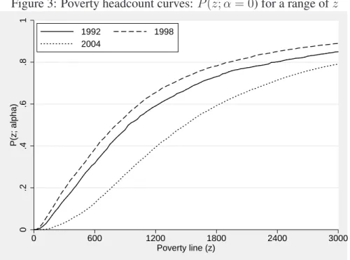
We begin our investigation by considering the evolution of the density of per capita incomes in Figure 1. The distribution of per capita income has worsened between 1992 and 1998 since the density curves have shifted to the left. It has however exhibited a strong and quick recovery between 1998 and 2004, as shown by the shift of the density curve to the right. The estimates of the Lorenz curves and Gini indices presented in Figure 2 and Table 1, respectively, suggest that in-equality has decreased between 1992 and 2004. Figures 3 and 4 and the results of Table 1 suggest that absolute poverty, as measured by the headcount and poverty gap indices, has increased between 1992 and 1998 and decreased between 1998 and 2004.
Table 1 also shows the sampling design effect for the estimation of average income per capita. The design effect is the ratio of the sampling-design-based estimate of the sampling variance (recall equation (34)) over the estimate of the sampling variance under the assumption of simple random sampling. For average income per capita, this stands to between 6.5 and 11. The ratio of standard
er-rors is therefore between around 2.5 and 3.3, which also suggests that it is quite important in our case to take into account sampling design in assessing sampling variability — otherwise, we would risk being much too imprudent in making in-ferences.
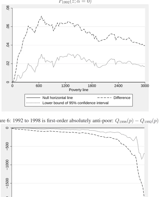
Formal statistical testing for first-order absolute pro-poorness of Mexican growth can be done using the information presented in Figures 5 to 10. The top line of Figure 5 shows the sample estimates of
∆1(z) = P
1998(z; α = 0) − P1992(z; α = 0) (36)
for the difference between 1998 and 1992, whereas the dotted bottom curve is the lower bound of the one-sided confidence interval,
∆1
0(z) − σ∆ˆs(z)ζ(θ). (37)
Since ∆1
0(z) − σ∆ˆs(z)ζ(θ) > 0 is verified on Figure 5 for all reasonable poverty
lines, we can infer from our data that growth was absolutely anti-poor during the period 1992 and 1998. The same result obtains from Figure 6 using differences in quantiles. The sample estimates of the difference in quantiles between 1992 and 1998 is shown by the dashed curve, and the upper bound of a one-sided confidence
interval is shown by the dotted curve. Since we can see on Figure 6 that ∆1
0(p) +
σ∆ˆs(p)ζ(θ) < 0 for all percentiles p between 0 and 0.95, we can again conclude from our data that growth was absolutely anti-poor during the period 1992 and 1998.
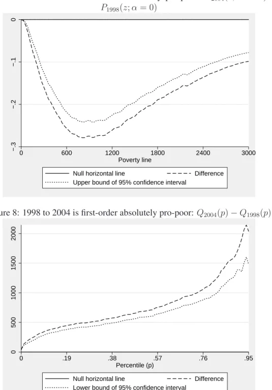
Opposite results are obtained when comparing 1998 to 2004. Judging from Figures 7 and 8, the change in distribution was first-order absolutely pro-poor. The
upper bound of the confidence interval for ∆1(z) is everywhere negative, whatever
reasonable poverty line is selected (remember that the official rural poverty line is 550 pesos per month per capita), and the lower bound of the confidence interval
for ∆1(p) is everywhere positive, whatever reasonable percentile is selected.
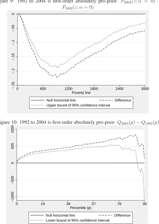
Given the conflicting results reported above, it would seem useful to check for pro-poorness over the entire period 1992 to 2004. This can be done using Figures 9 and 10. The distributive change was almost certainly first-order
abso-lutely pro-poor. The lower bound of the confidence interval for P2004(z; α = 0) −
P1992(z; α = 0) is everywhere negative, again whatever reasonable poverty line is
selected, and the lower bound of the confidence interval for the difference in
quan-tiles, Q2004(p) − Q1992(p), is everywhere positive, until at least the 0.8 percentile.
Thus, the anti-poor movement of 1992 to 1998 was outdone by the pro-poor move-ment of 1998 to 2004 so that the entire period of 1992 to 2004 can be inferred to be overall first-order absolutely pro-poor.
Given the robust results obtained for first-order pro-poorness, it is not useful to test for order pro-poorness since first-order pro-poorness implies second-order pro-poorness. This can be seen by noting that
Pj(z; α = 1) =
Z z
0
Pj(y; α = 0) dy. (38)
If first-order poorness obtains at order 1, then by (38) second-order pro-poorness also obtains. The same relation is obtained by noting from equations (7), (10) and (12) that the Generalized Lorenz curve condition is implied by the quantile condition.
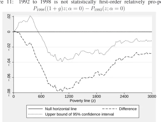
Testing for first-order relative pro-poorness can be done using Figures 11 to 20. Figure 11 shows why observing pro-poorness in samples does not mean that we can infer it in populations; to go from sample poorness to population pro-poorness, we need to apply statistical inference methods. To see this, note that despite the fact that average income fell by about 30% between 1992 and 1998,
the sample estimates of P1998((1 + g)z; α = 0) − P1992(z; α = 0) suggest that the
distributive movement during that period is first-order relatively pro-poor since that difference is always negative in the samples observed. But drawing a con-fidence interval around the sample estimates make it clear on Figure 11 that the
observed differences P1998((1 + g)z; α = 0) − P1992(z; α = 0) are not statistically
significant over a wide range of bottom poverty lines — the upper bounds of the one-sided confidence intervals extend above the zero line for z up to around 600 pesos and p up to around 0.28. Hence, with a conventional level 95% of statistical, the first-order relative pro-poor condition is not satisfied. An analogous result is obtained on Figure 12 from comparing growth in quantiles to growth in average income. Again, for a substantial range of percentiles, the one-sided confidence interval overlaps with the zero line.
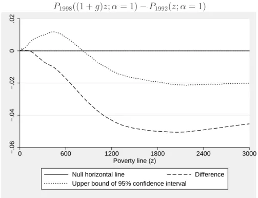
Moving to second-order relative pro-poorness does not help, as shown by Fig-ures 13 and 14. The statistical insignificance now extends over a wider range or z (up to around 900 pesos) and p (up to around 0.4) values. This may seem counter-intuitive at first sight, but it follows from the fact that statistical uncer-tainty for first-order comparisons at the bottom of the distributions builds up at the second-order since second-order conditions are made of cumulatives of first-order statistics (as discussed above). There is therefore an important lesson to be drawn here. If one were to omit testing for statistical significance, it might seem that second-order relative pro-poorness over the 1992-1998 period certainly can-not be weaker than first-order relative pro-poorness over the same period. But if
one takes into account the effect of sampling variability at the bottom of the dis-tribution, than the evidence for second-order relative pro-poorness is statistically weaker than that for first-order relative pro-poorness.
Testing for relative pro-poorness between 1998 and 2004 is more conclusive, as shown on Figures 15 and 16. The confidence interval around the sample
esti-mates of P2004((1 + g)z; α = 0) − P1998(z; α = 0) on Figure 15 is always below
zero for z up to around 1200 pesos (as opposed to 1800 pesos for the sample esti-mates), which leads us to infer a robust first-order relative pro-poorness change in that period. A similar result is obtained on Figure 16 from comparing growth in quantiles to growth in average income. For a range of percentiles up to about 0.7, the lower bound of the confidence interval lies above the zero line.
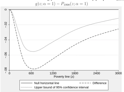
Given the above results, it would seem interesting to test for second-order relative pro-poorness for the 1998-2004 period. The results are shown on Figures 17 and 18. We now obtain even stronger (and very strong) evidence of the relative pro-poorness of that period. The confidence interval is always below zero for
differences P2004((1+g)z; α = 1)−P1998(z; α = 1) and above zero for differences
C2004(p)/C1998(p) − µ2004/µ1998. This is not surprising given that, as discussed
above, if first-order pro-poorness is verified statistically at order 1, then we can expect second-order pro-poorness also to be inferred statistically.
The results of the tests for relative pro-poorness over the period 1992 to 2004 are even stronger. These are shown on Figures 19 and 20. The confidence interval
around the sample estimates of P2004((1+g)z; α = 0)−P1998(z; α = 0) on Figure
19 is always below zero even as we extend z beyond 3000 pesos. The same strong evidence is displayed on Figure 16 from the comparison of growth in quantiles to growth in average income between 1992 and 2004. For a range of percentiles up to about 0.9, the lower bound of the confidence interval is everywhere above the zero line. Hence, the period 1992-2004 shows a statistically and ethically very robust degree of relative pro-poorness change in that period.
5 Conclusion
This paper proposes techniques to check for whether growth has been pro-poor. It first reviews different definitions of pro-poorness and argues for the use of methods that can generate results that are robust over classes of pro-poor measures and ranges of poverty lines. It then makes it empirically feasible to test for pro-poorness of growth. To do this, it derives the sampling distribution of the various estimators that are needed to test for absolute and relative pro-poorness. This
leads to the convenient use of confidence intervals around the curves that must be ranked in order to conclude that a change has been robustly pro-poor — or anti-poor.
These statistical techniques are then implemented using Mexico’s National Income and Expenditure Surveys collected in 1992, 1998 and 2004 and taking full account of the sampling design of these surveys. We find strong evidence that Mexican growth has been absolutely anti-poor between 1992 and 1998, absolutely poor between 1998 and 2004 and between 1992 and 2004, and relatively pro-poor between 1992 and 2004 and between 1998 and 2004. The assessment of the period between 1992 and 1998 is, however, statistically too weak to lead to a robust evaluation of this period, and this is true both for both first and second-order assessments of pro-poorness.
Table 1: Descriptive statistics
Statistics 1992 Year1998 2004
Sample size (households) 10530 10952 20595
Gini index 0.622 0.577 0.524
(0.017) (0.011) (0.010) Average income per capita 2115 1492 2430
(142) (69) (87) [6.52] [6.83] [10.88] µyear/µ1992 1.000 0.705 1.149 (0.000) (0.057) (0.087) Headcount index 0.291 0.354 0.106 (0.014) (0.022) (0.009) Average poverty gap 0.129 0.169 0.036
(0.009) (0.015) (0.004)
(...): Standard errors [...]: Sampling design effect
Figure 1: Density functions 0 .0002 .0004 .0006 .0008 f(y) 0 600 1200 1800 2400 3000
Income per capita (y)
1992 1998
2004
Figure 2: Lorenz curves
0 .2 .4 .6 .8 1 L(p) 0 .2 .4 .6 .8 1 Percentiles (p) 45° line 1992 1998 2004
Figure 3: Poverty headcount curves: P (z; α = 0) for a range of z 0 .2 .4 .6 .8 1 P(z; alpha) 0 600 1200 1800 2400 3000 Poverty line (z) 1992 1998 2004
Figure 4: Average poverty gap curves: P (z; α = 1) for a range of z
0 .2 .4 .6 P(z; alpha) 0 600 1200 1800 2400 3000 Poverty line (z) 1992 1998 2004
Figure 5: 1992 to 1998 is first-order absolutely anti-poor: P1998(z; α = 0) − P1992(z; α = 0) 0 .02 .04 .06 .08 0 600 1200 1800 2400 3000 Poverty line
Null horizontal line Difference
Lower bound of 95% confidence interval
Figure 6: 1992 to 1998 is first-order absolutely anti-poor: Q1998(p) − Q1992(p)
−2000 −1500 −1000 −500 0 0 .19 .38 .57 .76 .95 Percentile (p)
Null horizontal line Difference
Figure 7: 1998 to 2004 is first-order absolutely pro-poor: P2004(z; α = 0) − P1998(z; α = 0) −.3 −.2 −.1 0 0 600 1200 1800 2400 3000 Poverty line
Null horizontal line Difference
Upper bound of 95% confidence interval
Figure 8: 1998 to 2004 is first-order absolutely pro-poor: Q2004(p) − Q1998(p)
0 500 1000 1500 2000 0 .19 .38 .57 .76 .95 Percentile (p)
Null horizontal line Difference
Figure 9: 1992 to 2004 is first-order absolutely pro-poor: P2004(z; α = 0) − P1992(z; α = 0) −.25 −.2 −.15 −.1 −.05 0 0 600 1200 1800 2400 3000 Poverty line
Null horizontal line Difference
Upper bound of 95% confidence interval
Figure 10: 1992 to 2004 is first-order absolutely pro-poor: Q2004(p) − Q1992(p)
−1000 −500 0 500 1000 0 .19 .38 .57 .76 .95 Percentile (p)
Null horizontal line Difference
Figure 11: 1992 to 1998 is not statistically first-order relatively pro-poor: P1998((1 + g)z; α = 0) − P1992(z; α = 0) −.08 −.06 −.04 −.02 0 .02 0 600 1200 1800 2400 3000 Poverty line (z)
Null horizontal line Difference
Upper bound of 95% confidence interval
Figure 12: 1992 to 1998 is not statistically first-order relatively pro-poor: Q1998(p)/Q1992(p) − µ1998/µ1992 −.2 −.1 0 .1 .2 .02 .2 .38 .56 .74 .92 Percentile (p)
Null horizontal line Difference
Figure 13: 1992 to 1998 is not statistically second-order relatively pro-poor: P1998((1 + g)z; α = 1) − P1992(z; α = 1) −.06 −.04 −.02 0 .02 0 600 1200 1800 2400 3000 Poverty line (z)
Null horizontal line Difference
Upper bound of 95% confidence interval
Figure 14: 1992 to 1998 is not statistically second-order relatively pro-poor: C1998(p)/C1992(p) − µ1998/µ1992 −.2 −.1 0 .1 .2 .02 .2 .38 .56 .74 .92 Percentile (p)
Null horizontal line Difference
Figure 15: 1998 to 2004 is first-order relatively pro-poor: P2004((1 + g)z; α = 0) − P1998(z; α = 0) −.15 −.1 −.05 0 .05 0 600 1200 1800 2400 3000 Poverty line (z)
Null horizontal line Difference
Upper bound of 95% confidence interval
Figure 16: 1998 to 2004 is first-order relatively pro-poor: C2004(p)/C1998(p) −
µ2004/µ1998 −.5 0 .5 1 1.5 2 0 .19 .38 .57 .76 .95 Percentile (p)
Null horizontal line Difference
Figure 17: 1998 to 2004 is strongly second-order relatively pro-poor: P2004((1 + g)z; α = 1) − P1998(z; α = 1) −.08 −.06 −.04 −.02 0 0 600 1200 1800 2400 3000 Poverty line (z)
Null horizontal line Difference
Upper bound of 95% confidence interval
Figure 18: 1998 to 2004 is strongly second-order relatively pro-poor: C2004(p)/C1998(p) − µ2004/µ1998 0 .5 1 1.5 2 .02 .2 .38 .56 .74 .92 Percentile (p)
Null horizontal line Difference
Figure 19: 1992 to 2004 is first-order relatively pro-poor: P2004((1 + g)z; α = 0) − P1992(z; α = 0) −.15 −.1 −.05 0 0 600 1200 1800 2400 3000 Poverty line (z)
Null horizontal line Difference
Upper bound of 95% confidence interval
Figure 20: 1992 to 2004 is first-order relatively pro-poor: C2004(p)/C1992(p) −
µ2004/µ1992 0 .5 1 1.5 .02 .2 .38 .56 .74 .92 Percentile (p)
Null horizontal line Difference
References
ARAAR, A. (2006): “Poverty, Inequality and Stochastic Dominance, Theory
and Practice: Illustration with Burkina Faso Surveys,” CIRP ´EE Working Paper #0634.
BAHADUR, R. (1966): “A Note on Quantiles in Large Samples,” Annals of
Mathematical Statistics, 37.
BISHOP, J., J. FORMBY, AND P. THISTLE (1992): “Convergence of the
South and Non-South Income Distributions, 1969-1979,” American Eco-nomic Review, 82, 262–72.
BOURGUIGNON, F. (2003): “The poverty-growth-inequality triangle,” Tech.
rep., Paris, Agence franc¸aise de d´eveloppement.
BRUNO, M., M. RAVALLION, ANDL. SQUIRE(1999): “Equity and Growth
in Developing Countries: Old and New Perspectives on the Policy Is-sues,” SSRN Working Paper Series 604912.
DAVIDSON, R. AND J.-Y. DUCLOS (1997): “Statistical Inference for the
Measurement of the Incidence of Taxes and Transfers,” Econometrica, 65, 1453–65.
——— (2006): “Testing for Restricted Stochastic Dominance,” Cahier de recherche 06-09, CIRPEE.
DOLLAR, D.ANDA. KRAAY(2002): “Growth Is Good for the Poor,”
Jour-nal of Economic Growth, 7, 195–225.
DUCLOS, J.-Y. AND A. ARAAR (2006): Poverty and Equity
Measure-ment, Policy, and Estimation with DAD, Berlin and Ottawa: Springer and IDRC.
DUCLOS, J.-Y. AND Q. WODON(2004): “What is ”Pro-Poor”?” CIRP ´EE
Working Paper #0425.
EASTWOOD, R. AND M. LIPTON (2001): “poor Growth and
Pro-Growth Poverty Reduction: What do they Mean? What does the Evi-dence Mean? What can Policymakers do?” Asian Development Review, 19, 1–37.
ESSAMA-NSSAH, B. (2005): “A unified framework for pro-poor growth
KAKWANI, N., S. KHANDKER, AND H. SON (2003): “Poverty
Equiva-lent Growth Rate: With Applications to Korea and Thailand,” Tech. rep., Economic Commission for Africa.
KAKWANI, N.ANDE. PERNIA(2000): “What is Pro Poor Growth?” Asian
Development Review, 18, 1–16.
KLASEN, S. (2003): “In Search of the Holy Grail: How to Achieve Pro-Poor
Growth?” Discussion Paper #96, Ibero-America Institute for Economic Research, Georg-August-Universit¨at, Gttingen.
MCCULLOCH, N. AND B. BAULCH (1999): “Tracking pro-poor growth,”
ID21 insights #31, Sussex, Institute of Development Studies.
RAVALLION, M. AND S. CHEN (2003): “Measuring Pro-poor Growth,”
Economics Letters, 78, 93–99.
RAVALLION, M.ANDG. DATT(2002): “Why Has Economic Growth Been
More Pro-poor in Some States of India Than Others?” Journal of Devel-opment Economics, 68, 381–400.
SHORROCKS, A. (1983): “Ranking Income Distributions,” Economica, 50,
3–17.
SON, H. (2004): “A note on pro-poor growth,” Economics Letters, 82, 307–
314.
UNITED-NATIONS(2000): “A Better World for All,” Tech. rep., United
Na-tions, New York.
WORLD-BANK(2000): The Quality of Growth, New York: Oxford