Economic Policy when Models Disagree

Texte intégral

(1)2009s-03. Economic Policy when Models Disagree Pauline Barrieu Bernard Sinclair-Desgagné. Série Scientifique Scientific Series. Montréal Mars 2009. © 2009 Pauline Barrieu, Bernard Sinclair-Desgagné. Tous droits réservés. All rights reserved. Reproduction partielle permise avec citation du document source, incluant la notice ©. Short sections may be quoted without explicit permission, if full credit, including © notice, is given to the source..

(2) CIRANO Le CIRANO est un organisme sans but lucratif constitué en vertu de la Loi des compagnies du Québec. Le financement de son infrastructure et de ses activités de recherche provient des cotisations de ses organisations-membres, d’une subvention d’infrastructure du Ministère du Développement économique et régional et de la Recherche, de même que des subventions et mandats obtenus par ses équipes de recherche. CIRANO is a private non-profit organization incorporated under the Québec Companies Act. Its infrastructure and research activities are funded through fees paid by member organizations, an infrastructure grant from the Ministère du Développement économique et régional et de la Recherche, and grants and research mandates obtained by its research teams. Les partenaires du CIRANO Partenaire majeur Ministère du Développement économique, de l’Innovation et de l’Exportation Partenaires corporatifs Banque de développement du Canada Banque du Canada Banque Laurentienne du Canada Banque Nationale du Canada Banque Royale du Canada Banque Scotia Bell Canada BMO Groupe financier Caisse de dépôt et placement du Québec DMR Fédération des caisses Desjardins du Québec Gaz de France Gaz Métro Hydro-Québec Industrie Canada Investissements PSP Ministère des Finances du Québec Power Corporation du Canada Raymond Chabot Grant Thornton Rio Tinto Alcan State Street Global Advisors Transat A.T. Ville de Montréal Partenaires universitaires École Polytechnique de Montréal HEC Montréal McGill University Université Concordia Université de Montréal Université de Sherbrooke Université du Québec Université du Québec à Montréal Université Laval Le CIRANO collabore avec de nombreux centres et chaires de recherche universitaires dont on peut consulter la liste sur son site web. Les cahiers de la série scientifique (CS) visent à rendre accessibles des résultats de recherche effectuée au CIRANO afin de susciter échanges et commentaires. Ces cahiers sont écrits dans le style des publications scientifiques. Les idées et les opinions émises sont sous l’unique responsabilité des auteurs et ne représentent pas nécessairement les positions du CIRANO ou de ses partenaires. This paper presents research carried out at CIRANO and aims at encouraging discussion and comment. The observations and viewpoints expressed are the sole responsibility of the authors. They do not necessarily represent positions of CIRANO or its partners.. ISSN 1198-8177. Partenaire financier.

(3) Economic Policy when * Models Disagree Pauline Barrieu†, Bernard Sinclair-Desgagné ‡ Résumé / Abstract Ce texte propose une nouvelle approche du design des politiques publiques, quand il n'y pas de consensus entre experts sur une représentation adéquate de la situation. Techniquement parlant, nous adoptons pour ce faire une version généralisée de la théorie traditionnelle de la politique économique, telle que développée il y a plusieurs décennies par Jan Tinbergen. Contrairement aux solutions existantes à l'incertitude sur les modèles, notre approche ne demande pas de connaître la fonction d'utilité des décideurs politiques (à l'inverse de la littérature sur l'ambigüité), ni d'avoir un modèle de référence (par contraste avec la théorie du contrôle robuste), ni de posséder une distribution de probabilité sur l'ensemble des scénarios proposés (a contrario de l'approche bayesienne). Nous montrons que les politiques obtenues possèdent plusieurs propriétés que la littérature souvent postule a priori, comme la robustesse et la simplicité. Mots clés : Incertitude sur les modèles, théorie de la politique économique, ambigüité, robustesse. This paper proposes a general way to craft public policy when there is no consensual account of the situation of interest. The design builds on a dual extension of the traditional theory of economic policy. It does not require a representative policymaker’s utility function (as in the literature on ambiguity), a reference model (as in robust control theory) or some prior probability distribution over the set of supplied scenarios (as in the Bayesian modelaveraging approach). The obtained policies are shown to be robust and simple in a precise and intuitive sense. Keywords: Model uncertainty, Theory of economic policy, Ambiguity, Robustness Codes JEL : D80, E61, C60 *. We are grateful to Olivier Bahn, Arnaud Dragicevic, Claude Henry, Danny Ralph, Stefan Scholtes, and Michel Truchon for helpful conversations and suggestions. We also acknowledge valuable comments from seminar participants at HEC Montréal, the University of Strasbourg, and the Judge Business School/RAND “Modelling for Policy Advice” seminar series at the University of Cambridge. This paper was partly written while SinclairDesgagné was visiting the Judge Business School and the London School of Economics in academic year 20072008. † London School of Economics and Political Science. ‡ CIRANO and École polytechnique. HEC Montréal, International Economics and Governance Chair, HEC Montréal, 3000 chemin de la Côte-Sainte-Catherine, Montréal, Canada H3T 2A7; e-mail: bsd@hec.ca..

(4) We make to ourselves models of facts. - Ludwig Wittgenstein (1922) -. I. Introduction Models are an ever-present input of decision and policy making. Be they very sophisticated or not, they always are, however, partial representations of reality. The same object might therefore admit different models. Well-known current examples include global warming and its various impact assessment models, such as the DICE model conceived by William Nordhaus (1994) and the PAGE model used by Nicholas Stern (2007, 2008), and macroeconomic policy, with its competing DSGE models that respectively build on the New Keynesian framework (see, e.g., Richard Clarida et al., 1999; Michael Woodford 2003) or the Real Business Cycle view (see, e.g., Thomas Cooley 1995).1 Due to theoretical gaps, lack of data, measurement problems, undetermined empirical specifications, and the normal carefulness of modelers, such episodes of model uncertainty may often last beyond any useful horizon.2 Meanwhile, policymakers will be expected to act based on analyses, scenarios and forecasts which can be at variance from each other. 1. The “Dynamic Integrated model of Climate and the Economy” (DICE) is a global-economy model that explicitly considers the dynamic relationships between economic activity, greenhouse-gas emissions and climate change. The “Policy Analysis for the Greenhouse Effect” (PAGE), developed by Christopher Hope (2006), generates emission-reduction costs scenarios for four world regions, acknowledging that some key physical and economic parameters can be stochastic. There are many other models addressing the economics of global warming (see, e.g., Alan Manne et al. 1995; Nordhaus and Zili Yang 1996; Nordhaus and Joseph Boyer 2000; and Stern 2007, chapter 6). Most disagreements between climate change modellers have to do with discounting, technological innovation, and the treatment of risk and uncertainty (see, e.g., Geoffrey Heal 2008). Dynamic Stochastic General Equilibrium (DSGE) models, on their part, differ mainly in their microfoundations and the way they capture price and wage adjustments. 2. As Andrew Watson (2008, p. 37) recently pointed out, for instance: “In the foreseeable future (next 20 years) climate modelling research will probably not materially decrease the uncertainty on predictions for the climate of 2100. The uncertainty will only start to decrease as we actually observe what happens to the climate.” [Emphasis added]. 2.

(5) Economists have recently devoted significant efforts to assist policy making in this setting.3 Four approaches can be found in the literature at the moment: model averaging, discarding dominated policies, deciding under ambiguity, and robust control. The first one draws on Bayesian decision theory, thanks in part to new means for constructing a prior probability distribution (Adrian Raftery et al. 1997; Gary Chamberlain 2000; Carmen Fernandez et al. 2001; Antoine Billot et al. 2005). It has been advocated by a number of macroeconomists (see Christopher Sims 2002, William Brock et al. 2003, and the references therein). The second route, taken for instance by Charles Manski (2000) for the selection of treatment rules, avoids prior distributions altogether, seeking only policies that cannot be outdone in at least one model. The third approach acknowledges instead that several prior distributions might be plausible at the same time; it then develops decision criteria - such as Itzhak Gilboa and David Schmeidler (1989)’s maximin criterion or the more general adjusted-expected-utility criteria suggested respectively by Peter Klibanoff et al. (2005) and Fabio Maccheroni et al. (2006) - that fit reasonable patterns of behavior in this case (as they have been documented since Daniel Ellsberg 1961’s seminal article). Robust control, finally, builds on engineering (optimal control) methods for finding policies that will put up with any perturbation of a given reference model.4 It was persuasively introduced in macroeconomics by Lars Peter Hansen and 3 The first recognition of the importance of model uncertainty for the evaluation of macroeconomic policy actually dates back to William Brainard (1967). 4. In physics, a “perturbation” means a secondary influence on a system that causes it to deviate slightly. Hansen and Sargent (2008) define the word “slightly” as lying within a certain range of the reference model, where distance is measured by an entropy-based metric.. 3.

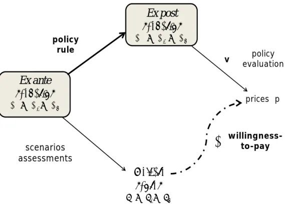
(6) Thomas Sargent (2001, 2008); some applications also exist in natural resources economics (see, e.g., Catarina Roseta-Palma and Anastasios Xepapadeas 2004). All these approaches, however, have some drawbacks. As argued by Andrew Levin and John Williams (2003), for instance, there might be no single reference model of the economy (since key issues such as expectations formation and inflation persistence still are controversial), which often makes robust control impractical. But the main alternatives Bayesian model-averaging or multiple-prior decision making - call for probabilistic beliefs over a collection of models or scenarios, which might also prove to be unrealistic in many settings. A major contribution of the recent literature on belief formation has actually been to identify situations in which entertaining probabilistic beliefs is hardly achievable or even rational (see Gilboa et al. (2008)’s recent survey on the subject).5 Besides, the available criteria for making decisions under ambiguity remain unsatisfactory: the maximin criterion really corresponds to an extreme form of uncertainty aversion, whereas the more general ones are not yet operational (especially to elicit and capture group preferences). Falling back on undominated policies, at last, will not be good enough, for such policies can be numerous and are allowed to do very poorly under some scenarios. Our goal in this paper is to set out a new approach which avoids these shortcomings. The proposed scheme, which is sketched in Figure 1, borrows several core elements (with some adjustments) from Jan Tinbergen (1952)’s theory of economic policy.6 A model 5 Enriqueta Aragonès et al. (2005) show that complexity, for example, can be one reason for this. A group of experts might also fail to hold a common prior if the set of models or scenarios is sufficiently large (see Martin Cripps et al. 2008). 6. For an historical perspective, literature review and appraisal, the reader may consult the successive. 4.

(7) brings together endogenous and exogenous variables, and some policy instruments (the short-term interest rate, say, or a carbon tax). Let different models involving the same policy instruments be simultaneously relevant to policymakers. For initial values of those instruments and the exogenous variables, each model  = 1   delivers a (possibly dynamic and stochastic) scenario or forecast   . In this context, a policy rule Φ is a prescription on the utilization of the policy instruments that prompts a revision of all scenarios. The challenge is to design an appropriate rule. Insert Figure 1 about here. Suppose that each original scenario   is given a welfare score  via a mapping , and that revised scenarios  01    0 must go through an overall policy assessment v(01   0 ) expressed in monetary units. Call a policy rule effective if its outcome receives a positive assessment whenever the score of at least one initial scenario did not meet some preestablished objective. We show in Section IV that an effective policy rule exists if and only if a shadow price (1    ) can be put on each configuration of scores so that v◦Φ = ◦ .. (1). This is a straightforward consequence of a generalization of Farkas’s Lemma - a statement central to linear programming and convex optimization - due to Bruce Craven (1972). Once the price schedule  is determined, a convenient policy Φ can then be obtained by solving equation (1). The scores  and assessment v should be regarded as intrinsic features of the policy articles by Andrew Hughes Hallett (1989), Ben van Velthoven (1990), Thráinn Eggertsson (1997), and Nicola Acocella and Giovanni Di Bartolomeo (2007).. 5.

(8) process, as opposed to subjective attributes of an imaginary individual planner. The former is indeed inherent to rule-based policies such as the Taylor Rule (proposed by John Taylor 1993) or the Kyoto Protocol, where they convey positive or negative deviations from some intended GDP level and inflation rate or some emission reduction target respectively. The latter may reflect the value or merit of policy outcomes to all members of an official board (perhaps following several discussion rounds, as reported for instance by Sims 2002 and Eric Leeper 2003). The shadow price , on the other hand, should be seen as expressing the policymakers’ willingness-to-pay for avoiding welfare levels in the range {1    }. Equation (1) thus says that a proper policy rule must make the value of its results match the willingness to escape the actual situation. To fix ideas further on this approach, the upcoming section gives a short example of what it can do in comparison to previous methods. The formal framework and general construction of policy rules are then laid out in Sections III and IV respectively. Key properties of these rules - such as self-restraint, non-neutrality, robustness, holism, and simpleness - are shown and discussed in Section V; note that these attributes are not postulated ex ante but are in fact derived from the construction. Section VI finally offers concluding remarks about implementation and some immediate extensions.. II. An Example Suppose there are two models of the economy, none of which is accepted as a benchmark.7 Each model  = 1 2 generates forecasts of aggregate wealth which take the form 7. This example is purely illustrative and has no pretence of realism. In Barrieu and Sinclair-Desgagné. 6.

(9) of normal distributions  ( − ; (1 − ) 2 ) with mean  −  and variance (1 − ) 2 . The parameters  and  2 are exogenous and specific to each model. The variable , which is scaled so as to belong to the interval [0 1], refers to variance-reducing policies that cost one unit of wealth per unit of decrease in volatility. Let 1  2 and  21   22 , so the first model predicts a larger average wealth but also greater volatility for any given policy . In order to apply the undominated-policies and model-averaging approaches, assume the policymakers’s preferences over wealth are representable using the constant-absoluterisk-aversion (CARA) utility function () = −− with coefficient of absolute risk aversion . It is well-known that ranking the forecasts of models  = 1 2 based on the expected values of a CARA utility function amounts to compare the certainty equivalents  () =  −  − . 2 (1 − ) 2 2 = ( −   ) + (  − 1) , 2 2 2. Undominated policies will then generally take the form  = 1 (if   = 0 (if . 2 2. 2 2.  = 1 2.  1 for some ) or.  1 for some ). Alternatively, a Bayesian policy maker who holds that. model 1 is right with prior probability  will choose  to maximize ∙ ¸  21  22 1 () + (1 − )2 () =   + (1 − ) − 1 + a constant 2 2 and be thereby lead to also select  = 0 or 1. When .  21 2.  1  1 and .  22 2.  1  2 ,. however, such dichotomous policies will perform rather badly under one model.8 (2006), we also explore a first specialized version of the method, which deals with diverging binary forecasts and uses linear shadow prices. 8 Obviously, the recommended policies took values 0 or 1 because we assumed the cost of policy was linear. Supposing instead a convex cost () could have resulted in solutions 0    1, but the contrasts we want to emphasize with other approaches to model uncertainty would then fade away.. 7.

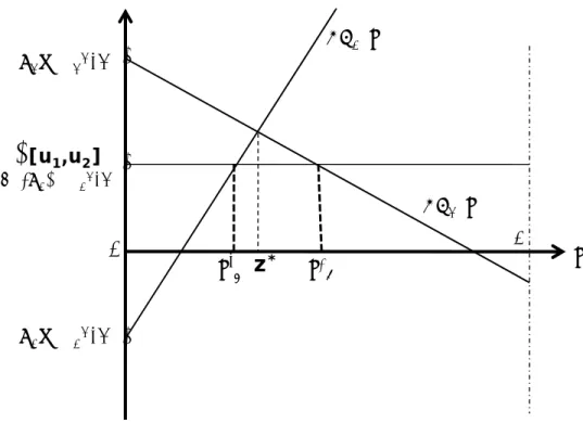
(10) In the latter case, by contrast, the maximin policy  ∗ sits at the intersection of the curves 1 () and 2 (), for any set of priors that includes  = 1 and  = 0. This action certainly limits the policy maker’s exposure to regrettable expected-utility outcomes if either scenario turns out to be the wrong one. But it may seem overly cautious to several people, especially if one model prefigures a very large return from modifying  ∗ slightly. Turning now to this paper’s approach, consider for simplicity the situation depicted 2. in Figure 2, where 1 ( ∗ )  −1 +  2 . Insert Figure 2 about here. Suppose  = 0 is the current policy, so the initial forecasts are in fact  = ( ;  2 ). Ascribe the welfare scores  =  − .  2 2. to these forecasts; let the revised scenarios be.  0 = ( − ; (1 − ) 2 ); and take v( 01   02 ). (1 − ) 21 (1 − ) 22 , 2 −  −  ] = min[1 −  −  2 2. as the ex post policy assessments. If the function (1  2 ) = − min[1  2 ] captures the policymakers’s willingness-to-pay to avoid the present welfare possibilities {1  2 }, then solving equation (1) amounts to seek a policy  • such that min[1 −  • − . (1 −  • ) 21 (1 −  • ) 22 2 2 , 2 −  • −  ] = − min[1 −  1 , 2 −  2 ] . 2 2 2 2. This yields two candidates • and • . These policies will not do as well as  ∗ in the worst case, of course. But their respective return will never be inferior to the policymakers’ subjective quote (1  2 ) to escape the present uncertain situation. In the above Figure, moreover, • produces a much higher reward if model 1 turns out to be right. 8.

(11) Policies like • and • could have been generated as well through the maximin approach, using a specific set of priors that excludes  = 0 and  = 1, or invoking one of the recent criteria for decision making under ambiguity. Our method, however, did not involve a selection of prior distributions (which might have required an infinite regress in beliefs) nor an exact encoding of ambiguity aversion. The scores  and policy evaluations v(01  02 ), moreover, should again be viewed as directly observable components of the policy process that may not have been derived from a particular utility function. We shall reflect further on this in the upcoming sections, where we make our construction more general and rigorous. III. The Basic Framework Suppose the scenarios or forecasts that can be supplied by a model (or an expert) belong to a set Ω. There is a total order over Ω, denoted ., which corresponds to the policymakers’ preferences over all scenarios: for any two scenarios  and w in Ω,  . w thus means that w is “preferable” to  from the policymakers’ viewpoint.9 When  . w but not w . , we write   w. Let the function  : Ω → R represent the policymakers’s preferences on a numerical scale, i.e.  . w if and only if () ≤ (w).10 9 A binary relation . defined over the set Ω is a total order if, for all , w, w◦ ∈ Ω, (i) either  . w or w .  (completeness property), (ii)  .  (reflexivity), (iii)  . w and w .  implies that  = w (antisymmetry), and (iv)  . w and w . w◦ implies that  . w◦ (transitivity). Property (iii) forbids that two different scenarios  6= w be equivalent (i.e. such that  . w and w . ). Accordingly, one may see the set Ω as made of collections of equivalent scenarios, each collection being represented by one of its elements.. A more general framework would have several sets Ω with respective total order . ,  = 1   (meaning that the range of possible forecasts and their ranking may depend on who the underlying model or expert are), while the function  takes values in a totally ordered (not necessarily numerical) set. The results shown below are still valid under these extensions. 10. 9.

(12) A. Multiple-Scenario Assessments From now on, there will be   1 different models, noted 1    , drawn from a set . At a given time, the policymakers is then presented a variety of forecasts  = ( 1   2     ) which belong to the cartesian product Ω . The order relation . can be applied componentwise to obtain the canonical partial order ¹ on Ω :  ¹ w if and only if   . w. for all  = 1   .. If    w for all  = 1  , we write  ≺ w. One can also construct the assessment function  : Ω → R as () = ((1 )  ( )) = (1    ). Let Σ =  (Ω ) ⊆ R denote the image of . Note that, by definition, the function  : Ω → Σ is surjective. B. Policy Rules Without loss of generality, the number 0 will be seen as a threshold or target for policy intervention.11 If Σ− = Σ \ R+ = { = (1    ) ∈ Σ :   0 for some }, then each element of the set Ω− =  −1 (Σ− ) contains at least one scenario policymakers deem bad enough to warrant some remedial action. Assume that a single action (which may itself involve the simultaneous or sequential deployment of several policy instruments) is undertaken at a time, and that each expert or model is able in this case to provide a revised scenario. Policy intervention can then be portrayed as a function Φ : Ω → Ω such that Φ() = 0 captures its impact (according to the same  models or experts)  0 = (01   02    0 ) on all the initial scenarios ( 1  2    ) comprised in . In what follows, we refer to Φ as a policy rule. 11. This threshold is chosen for convenience only. Our results would not be altered by setting a different target ◦ in R.. 10.

(13) C. Policy Evaluation Modified scenarios and forecasts are finally subject to overall appraisals. These are given by the function v: Ω → , where  is a set of real numbers. Below, we denote + the intersection  ∩ R+ . In their account of monetary policy, Levin and Williams (2003, p. 946) suggest that a policymaking committee usually seeks policy outcomes that are acceptable to all its members. In agreement with this stylized fact, the function v will be supposed to meet the following assumption. Assumption 1 (Unanimity).  ∈ Ω− ⇔ v() ≤ 0 . In other words, policies that perform very poorly in at least one of the committee members’ model and thus fail to be consensual will receive a nonpositive score. Let  : Ω → R denote the composition  = v ◦ Φ of the functions v and Φ. Given Assumption 1, it can be understood as the policymakers’ willingness-to-accept a modification of the initial scenarios through the policy rule Φ. This completes the background necessary to lay out our general approach to policy design under model uncertainty.. IV. A General Method for Policy Making The foundation of our approach is the following adaptation to the actual notation and context of a theorem demonstrated in Craven (1972; theorem 2.1). This theorem is a nonlinear generalization of the well-known Farkas’s Lemma of convex analysis.. 11.

(14) Theorem: If  : Ω → Σ is surjective, then  () =  (w) ⇒  () =  (w) and. (2).  () ∈ Σ− ⇒  () ∈ +. (3). if and only if there exists a function  : Σ →  such that =◦. and (Σ− ) ⊂ + .. (4). The above framework ensures that the theorem’s premises are satisfied.12 A policy rule Φ that fulfills condition (3) can be called effective; it amends any combination of bad scenarios so that no further intervention is needed. Condition (2) is one of consistency: scenarios which get the same rankings trigger equivalent policies (from the policymakers’ standpoint). Of course, one may have Φ () 6= Φ (w) but  () =  (w), so this condition does not exclude applying different treatments to similar scenarios (as the above example illustrates). Condition (2) does not apply, moreover, to situations where w is a permutation of , for in this case  () 6=  (w) most of the time; the identity of an expert who supports a given scenario may thus matter for policy. Since (Σ− ) ⊂ + , so (1    ) is positive whenever an initial scenario  is bad (  0 for some ), the “dual” function  can be typically interpreted as indicating the “price” policymakers are willing to pay to avoid an original set of scenarios {1    }. The theorem then says that a consistent and effective policy rule must be such that the policymakers’ willingness-to-accept its impact  = v ◦ Φ matches their willingness-to-pay  ◦  to escape the initial forecasts. The proof of this statement now follows. 12. If Ω , Σ and  are topological spaces,  is a continuous open map and  is continuous, one can also show that the price schedule  is continuous (see Craven 1972).. 12.

(15) Proof (Craven 1972): Suppose that conditions (2) and (3) are true. Then, for each  ∈ Σ, let () = (), where  is any element of Ω such that () = . Condition (2) ensures that  is a well-defined function. Furthermore, its domain is Σ, since (Ω ) = Σ, and  =  ◦  by definition. If  ∈ Σ− , then  = () for some  ∈ Ω− , and (3) entails  () ∈ Σ− ⇒  () = () ∈ + , so  (Σ− ) ⊂ + . Conversely, let  : Σ →  satisfy (4); the function  defined as  = ◦ obviously meets (2) and (3). ¥ This theorem justifies seeking a suitable policy Φ by solving the fundamental equation v◦Φ = ◦ .. (1). The construction relies on the mappings  and v, which represent ex ante and ex post assessments. Such devices seem to be natural components of any working policy process. They may not usually take explicit functional forms, of course, but the functions  and v, being very general, should fit most common practices. The approach also chiefly involves the policymakers’ willingness-to-pay . Although eliciting the latter may not be straightforward, it is generally easier than assessing utility functions, and there is a vast literature plus a wealth of concrete experience on the subject.13 Knowing  , v and , one can find Φ by solving equation (1) directly, as in the example of Section II, or by taking a quasi-inverse v[−1] of v so that14 Φ = v[−1] ◦  ◦  . 13. (5). Covering this literature and its applications is certainly beyond the scope of this paper. Let us simply point out that at least one leading procedure - the so-called BDM mechanism (or one of its variants) proposed initially by Gordon Becker et al. (1964) - might be applicable here. 14 The mapping v[−1] :  → Ω is a quasi-inverse of v if v ◦ v[−1] ◦ v = v. Every function has a quasi-inverse (if the Axiom of Choice holds). Yet, v[−1] is not unique unless v is a bijection. Note that v[−1] can be a quasi-inverse of v but not vice versa; this fact must be dealt with in order to use (5).. 13.

(16) To make sure that  fully agrees with the present interpretation, one may replace the theorem’s condition that (Σ− ) ⊂ + with the following stronger requirement. Assumption 2 (Strict willingness-to-pay).  ∈ Σ− ⇔  ()  0 . As we shall now see, policy rules built with shadow prices  that satisfy the latter have appealing characteristics.. V. Some Key Economic Properties of Policy Rules The literature on model uncertainty normally stipulates a priori that the designed policy rules possess certain desirable properties. One such property is robustness, which calls for policies that may not be optimal under some models but that will be acceptable if any of the ex post scenarios materializes (see, e.g., Hansen and Sargent 2008). Another one is simpleness, which is often understood as having policies that depend on a restricted set of variables (see, e.g., Denise Côté et al. 2002). This section shows that our approach actually endows the obtained policy rules with these properties, and other valuable ones. One pleasing attribute of a policy rule Φ which solves equation (1) is that it eliminates all the bad initial scenarios and never induces an unfavorable one. Hence, when a model  initially renders a forecast  so that ( )  0, nobody would oppose applying the rule.  Ω− . Property 1 (Consensual remedy): For all  ∈ Ω− , Φ () ∈ Proof: Suppose there exists some  ∈ Ω− with Φ () ∈ Ω− . By Assumption 1, we must have that v ◦ Φ() ≤ 0. However, since  ∈ Ω− , () ∈ Σ− and  ◦ ()  0 by Assumption 2. This contradicts the fact that v ◦ Φ() =  ◦ (). ¥. 14.

(17) By contrast, policy intervention will not receive unanimous support when all initial scenarios are good, for it will give rise to at least one bad forecast. Property 2 (Self-restraint): Let Ω+ = Ω \ Ω− . For all  ∈ Ω+ , Φ () ∈  Ω+ . Proof: Assume there exists some  ∈ Ω+ with Φ () ∈ Ω+ . By Assumption 1, we must have that v ◦ Φ()  0. However, since  ∈ Ω+ , () ∈ Σ \ Σ− and  ◦ () ≤ 0 by Assumption 2. This contradicts the fact that v ◦ Φ() =  ◦ (). ¥ A direct consequence of these properties is that Φ does not have a fixed point. This means that no policy intervention is without consequences on the ex post scenarios. Property 3 (Non neutrality): For all  ∈ Ω , Φ () 6=  . This third property may serve as a warning on policymakers to use the policy rule wisely. It may alternatively be viewed as a rough safeguard against indifferent or stubborn experts who could unduly maintain their initial forecast.. A. Robustness If one is ready to assume that the set Ω , partially ordered by ¹, is a complete lattice, Property 3 combined with the fixed-point theorems of lattice theory (see Brian Davey and Hilary Priestley 2002, theorems 8.22 and 8.23) implies that the policy rule Φ is neither order-preserving (or monotone) nor all-improving (the latter meaning that  ≺ Φ () for all  ∈ Ω ).15 The latter property happens to be true, moreover, on the very domain Ω− where policy intervention is needed. 15. Recall that (Ω  ¹) is a complete lattice if every subset of Ω has a least upper bound (supremum) and a greatest lower bound (infimum) in Ω .. 15.

(18) Property 4 (Imperfect enhancement): For at least one  ∈ Ω− , we have that  ⊀ Φ (). Proof: Suppose instead that  ≺ Φ () for all  ∈ Ω− . Let Ω− = { = (1    ) ∈ Ω | (  ) =   0 for all  6= 1}. Since Ω is a complete lattice, the set Ω− has a supremum ∨Ω− =   = (1     ). Clearly, (  ) =   0 for all  6= 1, so  ∈ Ω− . Taking Φ( ), consider now the n-tuple  4 = (Φ1 (  )  2     ) which differs from   in having the first component of the latter replaced by the first component Φ1 ( ) of Φ(  ). Such a n-tuple also belongs to Ω− , so we must have that Φ1 ( 4 ) .  1 . This inequality contradicts our initial assumption. ¥ This property could be observed in the example of Figure 2, where we had (02 ) = 2 − • −. (1− • ) 22 2.  2 −. 22 2. = ( 2 ). Together with Property 1, it captures the meaning. of robustness: the policy rule Φ fulfills its objectives in taking care of the unwelcome original scenarios, sometimes at the expense of the good ones (hence in a nonoptimal way with respect to some models), but never to the point of changing the latter into bad ones. Properties 1 and 4 suggest in addition that solving equation (1) provides a means of crafting precautionary policies.16 Reporting on the Federal Reserve Chairman’s conference to the 2004 annual meeting of the American Economic Association, Carl Walsh (2004) defines indeed a precautionary policy as one that “would err on the side of reducing the chance that the more costly outcome occurs.” Satisfying the maximin criterion was then seen as a practical way to bring about such a policy. Our approach now offers a distinct alternative, which also gives priority, but not exclusive attention, to the worst cases. 16. See Barrieu and Sinclair-Desgagné (2006) for further discussion on this point and the related implementation of the so-called Precautionary Principle.. 16.

(19) B. Simpleness The use of simple policy prescriptions, given the inherent complexity of the economy and the ensuing uncertainty of policymakers, was already advocated decades ago by Milton Friedman (1968). Since that time, simpleness is often conceived as a desideratum that precludes policies from fine-tuning the scenarios predicted by a specific model. As it turns out, solutions Φ to equation (1) do comply with this requirement, in a precise sense. Call a policy rule Γ : Ω → Ω decomposable if there exist some functions   : Ω → Ω  = 1   such that Γ() = ( 1 ( 1 )    ( )) for all  = (1    ) ∈ Ω .17 Clearly, policies which finely adjust to the peculiarities of each model must be decomposable. A policy Φ constructed as above will not be like this. Property 5 (Holism): The policy rule Φ : Ω → Ω is not decomposable. Proof: Suppose instead that Φ() = (1 (1 )   (  )) for all  = ( 1     ) ∈ Ω . Take now some  ¦ = ( ¦1    ¦ ) ∈ Ω+ so that (1 (¦1 ))  0, and consider an n-tuple  ∇ = (¦1   2     ) where (  )  0. We then have that Φ( 5 ) = (1 ( ¦1 )   ( )) with 1 (¦1 )  0, which contradicts Property 1. ¥ Property 5 suggests that Φ might ignore, at least partially in a certain range, the values taken by some endogenous or exogenous variables in a specific scenario. On a different note, it underscores the effect an upstream decision (based on strategic or epistemological considerations) to let a model in or not may have on policy design.. 17. This is a stronger form of decomposability. In mathematics and computer science, the decomposition of a multivalued function Γ : Ω → Ω involves some functions  1     : Ω → Ω and Λ : Ω → Ω such that Γ() = Λ( 1 ()    ()) for all  ∈ Ω .. 17.

(20) VI. Conclusion In the presence of model uncertainty, having a policy process which formally assesses ex ante forecasts and ex post policy outcomes suffices for developing a policy rule, provided one is able to elicit the policymakers’ willingness-to-pay to avoid the configuration of welfare levels projected initially. Under unanimous decision making and strict willingnessto-pay, moreover, the obtained policy rule will have a number of desirable properties, such as consistency, self-restraint, robustness, and simpleness. At least three issues must be dealt with before these conclusions are assured to hold in practice. First, one needs to understand how political and strategic factors might distort the observed assessments and declared willingness-to-pay. Given its influence on policy design, the set of relevant models might also be targeted by some interested parties. Handling these concerns satisfactorily does not seem implausible, however, since the classical theory of economic policy, which underlies the present framework, has already been extended from a single decision-maker context to a strategic multiple-player one (see Acocella and Di Bartolomeo 2006). Secondly, one ought to analyze a dynamic version of the current scheme, which allows models to evolve and policymakers to learn (something proponents of model averaging or the ambiguity criteria have already done). A first step in this direction would be to consider what happens to the policy rule Φ when the set of scenarios Ω shrinks or expands. Finally, the true scenario might not be among the supplied ones. This case remains a puzzle for the Bayesian and ambiguity approaches, which rely on probability distributions.. 18.

(21) Our method, on the other hand, might adequately come to terms with it because beliefs concerning whether or not at least one forecast can be trusted should be embedded in the shadow price . This point calls again for further investigation. References Acocella, Nicolas, and Giovanni Di Bartolomeo. 2007. “Toward a New Theory of Economic Policy: Continuity and Innovation.” Mimeo, University of Teramo. Acocella, Nicolas, and Giovanni Di Bartolomeo. 2006. “Tinbergen and Theil Meet Nash: Controllability in Policy Games.” Economics Letters, 90: 213-218. Aragonès, Enriqueta, Itzhak Gilboa, Andrew W. Postlewaite, and David Schmeidler. 2005. “Fact-Free Learning.” American Economic Review, 95(5): 1355-1368. Barrieu, Pauline, and Bernard Sinclair-Desgagné. 2006. “On Precautionary Policies,” Management Science, 52(8): 1145-1154. Becker, Gordon M., Morris H. DeGroot, and Jacob Marschak. 1964. “Measuring Utility by a Single-Response Sequential Method,” Behavioral Science, 9(3): 226-32. Billot, Antoine, Itzhak Gilboa, Dov Samet, and David Schmeidler. 2005. “Probabilities as Similarity-Weighted Frequencies.” Econometrica, 73(4): 1125-1136. Brainard, William C. 1967. “Uncertainty and the Effectiveness of Policy.” American Economic Review, 57(2): 411-425. Brock, William A., Steven N. Durlauf, and Kenneth D. West. 2003. “Policy Evaluation in Uncertain Economic Environments.” Brookings Papers on Economic Activity, 2003(1): 235-301. Chamberlain, Gary. 2000. “Econometrics and Decision Theory.” Journal of Econometrics, 95(2): 255-283. Clarida, Richard, Jordi Gali, and Mark Gertler. 1999. “The Science of Monetary Policy: a New-Keynesian Perspective.” Journal of Economic Literature, 37: 1661-707. Cooley, Thomas, ed. 1995. Frontiers of Business Cycle Research. Princeton, NJ: Princeton University Press. Côté, Denise, Jean-Paul Lam, Ying Liu, and Pierre St-Amant. 2002. “The Role of Simple Rules in the Conduct of Canadian Monetary Policy.” Bank of Canada Review, Summer 2002: 27-35. Craven, Bruce D. 1972. “Nonlinear Programming in Locally Convex Spaces.” Journal of Optimization Theory and Applications, 10(4): 197-210. Cripps, Martin W., Jeffrey C. Ely, George J. Mailath, and Larry Samuelson. 2008. “Common Learning.” Econometrica, 76(4): 909-933.. 19.

(22) Davey, Brian A., and Hilary A. Priestley. 2002. Introduction to Lattices and Order (second edition). Cambridge, UK: Cambridge University Press. Eggertsson, Thráinn. 1997. “The Old Theory of Economic Policy and the New Institutionalism.” World Development, 25(8): 1187-1203. Ellsberg, Daniel. 1961. “Risk, Ambiguity, and the Savage Axioms,” Quarterly Journal of Economics, 75 (4): 643—669 Fernandez, Carmen, Eduardo Ley, and Mark F. J. Steel. 2001. “Benchmark Priors for Bayesian Model Averaging,” Journal of Econometrics, 100: 381-427. Friedman, Milton. 1968. “The Role of Monetary Policy,” American Economic Review, 58(1): 1-17. Gilboa, Itzhak, Andrew Postlewaite, and David Schmeidler. 2008. “Probability and Uncertainty in Economic Modelling.” Journal of Economic Perspectives, 22(3): 173-188. Gilboa, Itzhak, and David Schmeidler. 1989. “Maximin Expected Utility with Non Unique Prior,” Journal of Mathematical Economics, 18: 141-153. Hansen, Lars Peter, and Thomas J. Sargent. 2001. “Robust Control and Model Uncertainty.” American Economic Review, 91(2): 60-66. Hansen, Lars Peter, and Thomas J. Sargent. 2008. Robustness. Princeton, NJ: Princeton University Press. Heal, Geoffrey. 2008. “Climate Economics: A Meta-Review and Some Suggestions for Future Research.” Review of Environmental Economics and Policy, published online at http://reep.oxfordjournals.org/cgi/content/short/ren014v1. Hope, Christopher. 2006. “The Marginal Impact of CO2 CH4 and SF6 Emissions,” Climate Policy, 6(5): 537-544. Hughes Hallett, Andrew J. 1989. “Econometrics and the Theory of Economic Policy: The Tinbergen-Theil Contributions 40 Years On.” Oxford Economic Papers, 41(1): 189-214. Klibanoff, Peter, Massimo Marinacci, and Sujoy Mukerji. 2005. “A Smooth Model of Decision Making under Ambiguity,” Econometrica, 73(6): 1849-1892. Leeper, Eric M., and Thomas J. Sargent. 2003. “[Policy Evaluation in Uncertain Economic Environments]. Comments and Discussion.” Brookings Papers on Economic Activity, 2003(1): 302-322. Levin, Andrew T., and John C. Williams. 2003. “Robust Monetary Policy with Competing Reference Models,” Journal of Monetary Economics, 50: 945-975. Maccheroni, Fabio, Massimo Marinacci, and Aldo Rustichini. 2006. “Ambiguity Aversion, Robustness, and the Variational Representation of Preferences,” Econometrica, 74(6): 14471498.. 20.

(23) Manne, Alan, Robert Mendelsohn, and Richard Richels. 1995. “MERGE - A Model for Evaluating Regional and Global Effects of GHG Reduction Policies,” Energy Policy, 23(1): 17-34. Manski, Charles F. 2001. “Identification Problems and Decisions under Ambiguity: Empirical Analysis of Treatment Response and Normative Analysis of Treatment Choice.” Journal of Econometrics, 95(2): 415-442. Nordhaus, William D. 1994. Managing the Global Commons. The Economics of Climate Change. Cambridge, MA: MIT Press. Nordhaus, William D., and Joseph G. Boyer. 2000. Warming the World: Economic Models of Global Warming. Cambridge, MA: MIT Press. Nordhaus, William D., and Zili Yang. 1996. “A Regional Dynamic General-Equilibrium Model of Alternative Climate-Change Strategies.” American Economic Review, 86(4): 741765. Raftery, Adrian E., David Madigan, and Jennifer A. Hoeting. 1997. “Bayesian Model Averaging for Linear Regression Models.” Journal of the American Statistical Association, 92(437): 179-191. Roseta-Palma, Catarina, and Anastasios Xepapadeas. 2004. “Robust Control in Water Management.” Journal of Risk and Uncertainty, 29(1): 21-34. Sims, Christopher A. 2002. “The Role of Models and Probabilities in the Monetary Policy Process.” Brookings Papers on Economic Activity, 2002(2): 1-40. Stern, Nicholas. 2008. “The Economics of Climate Change,” American Economic Review, 98(2): 1-37. Stern, Nicholas. 2007. The Economics of Climate Change: The Stern Review. Cambridge, UK: Cambridge University Press. Taylor, John B. 1993. “Discretion versus Policy Rules in Practice.” Carnegie-Rochester Conference Series on Public Policy, 39: 195-214. Tinbergen, Jan. 1952. On the Theory of Economic Policy (sixth printing). Amsterdam, North Holland Publishing Company. van Velthoven, Ben C. J. 1990. “The Applicability of the Traditional Theory of Economic Policy.” Journal of Economic Sur veys, 4(1): 59-88. Walsh, Carl E. 2004. “Precautionary Policies,” Federal Reserve Bank of San Francisco Economic Letter, 2004-05: 1-2. Wittgenstein, Ludwig. 1922. Tractatus Logico-Philosophicus. London: Routledge and Kegan Paul Ltd. Woodford, Michael. 2003. Interest and Prices: Foundations of a Theory of Monetary Policy. Princeton, NJ: Princeton University Press.. 21.

(24) . Ex post scenarios policy rule. Φ. ω1' … ωi' … ωn' v. Ex ante scenarios. prices p. ω1 … ωi … ωn. π. scenarios U assessments. welfare scores u1 … ui … u n Figure 1. The basic construction . policy evaluation. willingnessto-pay.

(25) . a2–ασ2. 2/2. π[u1,u2]. CE1(z). ▪. •. = -a1+ασ12/2. ▪. 0. CE2(z) 1 z◦A. z*. z●B. z. a1–ασ12/2 ▪. Figure 2. The maximin and this paper’s solutions. .

(26)