Heterogeneous vortex dynamics in high temperature superconductors

(1)

HAL Id: tel-00467466

https://pastel.archives-ouvertes.fr/tel-00467466

Submitted on 26 Mar 2010

HAL is a multi-disciplinary open access

archive for the deposit and dissemination of sci-entific research documents, whether they are pub-lished or not. The documents may come from teaching and research institutions in France or abroad, or from public or private research centers.

L’archive ouverte pluridisciplinaire HAL, est destinée au dépôt et à la diffusion de documents scientifiques de niveau recherche, publiés ou non, émanant des établissements d’enseignement et de recherche français ou étrangers, des laboratoires publics ou privés.

superconductors

Feng Yang

To cite this version:

Feng Yang. Heterogeneous vortex dynamics in high temperature superconductors. Superconductivity [cond-mat.supr-con]. Ecole Polytechnique X, 2009. English. �tel-00467466�

(2)

Thèse pour obtenir le grade de

DOCTEUR DE L’ÉCOLE POLYTECHNIQUE

Specialité : Physique

par

Feng YANG

Heterogeneous vortex dynamics

in high temperature superconductors

Soutenue le 18 juin 2009 devant le jury composé de :

Gilles Montambaux Président Rinke J. Wijngaarden Rapporteur

Alain Pautrat Rapporteur Takasada Shibauchi Examinateur

Julien Bobroff Examinateur Kees van der Beek Directeur

Thèse préparée au Laboratoire des Solides Irradiés,

Ecole Polytechnique, 91128 Palaiseau, France.

(3)

(4)

(5)

(6)

Remerciements

Je tiens à remercier Guillaume Petite et Martine Soyer, pour leurs accueils chaleureux et leurs encouragements constants pendant toute la durée de la réalisation de cette thèse au Laboratoire des Solides Irradiés (LSI, CEA-CNRS-Ecole Polytechnique, UMR 7642) où ils président. J’exprime mes sincères remerciements à Rinke J. Wijngaarden et Alain Pautrat qui ont accepté d’être mes rapporteurs, ainsi qu’à Gilles Montambaux, Takasada Shibauchi, Julien Bobroff et Kees van der Beek, d’avoir accepté de faire partie de mon jury de thèse.

Marcin Konczykowski, chef du groupe "supraconductivité et matériaux nanostruc-turés" au LSI jusqu’en avril 2009, je te remercie pour ton aide et tes conseils précieux dans la réalisation de ma thèse, ainsi que pour tes efforts d’animation de notre groupe dont j’ai bénéficié.

Kees van der Beek, mon directeur de thèse, je te suis reconnaissant de m’avoir en-seigné les techniques de mesures physiques, et la physique de vortex, et de m’avoir fait partager ta vision de la recherche scientifique.

Tout au long de cette thèse, j’ai bénéficié d’un environnement de collaboration scien-tifique de proximité et internationale. En voici un aperçu chronologique :

Mon premier contact avec la magnéto-optique se fait par Iryna Abal’osheva, de l’Insti-tut de Physique à Varsovie (Académie des Sciences de Pologne), pendant sa visite au LSI au sujet d’un film magnétique. Piotr Gierlowski, membre de ce même institut, a élaboré les masques de nickel, éléments indispensables pour créer la structure "canaux" par l’irradiation aux ions lourds.

Les échantillons de BSCCO sur lesquels j’ai travaillé sont fournis par Peter H. Kes et Ming Li, du laboratoire Kamerlingh Onnes, de l’Universiteit Leiden, Pays-Bas. Le travail présenté en Chapitre 4 de ce manuscrit est à l’initiative de Yuji Matsuda et Takasada Shibauchi, de l’Université de Kyoto. Le monocristal YBCO de haute qualité, utilisé dans cette étude, est fourni par Bogdan Dabrowski, de Northern Illinois University.

Comment ne pas remercier deux chercheurs de l’Unité Mixte de Physique CNRS/Tha-les (UMR 137) : Rozenn Bernard et Javier Briatico? C’est grâce à leur aide précieuse en photolithographie que le courant a enfin pu être injecté correctement dans les monocristaux de BSCCO irradiés.

Tatiana Taurines, élève-ingénieur de Supélec, a réalisé des mesures des magnéto-5

(7)

optiques différentielles pour moi sur les cristaux BSCCO "24-4", BSCCO "iv", et BSCCO "17" pendant son stage de 2`eme année d’ingénieur alors que j’étais occupé à la rédaction de ma thèse. Une partie des images magnéto-optiques présentées dans le Chapitre 5 de ce mémoire sont les fruits de son travail. C’est plus tard1 que je me suis rendu compte de l’importance des mesures que Tatiana Taurines a réalisées. Comme promis, je lui ferai parvenir ce manuscrit. Je lui exprime mes sincères remerciements pour ses mesures.

En quelques années, je suis passé du statut d’étudiant insouciant à celui de doctorant préparant sa soutenance. Cette expérience m’inspire ces quelques réflexions :

1. Il ne faut pas laisser traîner une chose trop longtemps.

Peut-être on peut inspirer de vivre chaque jour comme le dernier jour? 2. "Fail to plan is to plan to fail".

3. Comment transformer les idées émanant de "chercheur-amateur" par l’approche d’un "chercheur-confirmé"?

Souvent un amateur est très libre dans sa pensée et il émet des idées intéressantes mais souvent fausses ou simplistes. Peut-être 1 sur 10 peut franchir la première étape de questionnement, et mérite d’être étudiée avec plus de soin. A partir de ce moment là, c’est l’approche standard et rigoureuse qu’il faut employer pour l’examiner. Je suis encore un débutant et pour moi, il y a encore un long chemin à faire pour mériter la qualification de "chercheur-confirmé".

Je remercie à Travis d’avoir relu une partie de ce mémoire et corrigé mes fautes d’anglais. Je dois à Kees son aide précieuse dans différentes phases de rédaction de ce manuscrit. Panayotis, je pense à te retrouver bientôt au LSI et je te souhaite beaucoup de bonnes choses pour toi. Je remercie à tous les membres du LSI qui ont contribué à une bonne ambiance et une convivialité d’y travailler.

Mes remerciements vont également à tous mes amis qui se trouvent en dehors du laboratoire : à mes amis de promotion (Fatima, Alix, Julien, Olivier, Thibault, Nicolas, Johannès et Eric) avec qui nous avons laissé nos traces en France, en Espagne, en Chine, et bientôt on fera la route de la soie? A ma communauté chinoise à qui j’ai toujours la joie de penser (pas seulement pour la douceur de sa cuisine) : WANG Minmin, REN Jizhao, WU Han, HE Mi, ZHOU Bing, YU Linwei, YU Guosheng, ... aussi à mes amis chinois qui ne se trouvent pas ou plus sur le plateau : ZHANG Jin, HUO Jie, LI Yuan, 1 _{J’ai en effet remarqué que les trois faits suivants sont cohérents et se soutiennent mutuellement : (1) les} plots irradiés à basses températures résistent plus au champ magnétique; (2) la résistance de l’échantillon de BSCCO (contenant les plots irradiés) est linéaire; (3) l’imagerie de circulation du courant a montré que le courant contourne les plots irradiés. A haute température (proche de Tc), la situation est exactement inverse, et cela est également confirmé par toutes les mesures (magnéto-optique différentielle avec modulation en champ et la non-linéarité de la résistance à ce régime proche de Tc).

(8)

7 JIAO Chenyu, HE Yuchan, ZHOU Feng, ZHENG Jin, TAN Xiaolu, XIA Lian, ZHOU Guodong, CHEN Huayi, JIAO Ying, JIN Ming, ... à mes amis avec qui je peux oublier la barrière linguistique et culturelle : Ermias, Giulia, Pedro et Raffaella, et à tous les autres que je n’ai pas mentionné ici.

Je tiens à remercier personnellement Roland Sénéor pour son soutien sans faille, à Christoph Kopper pour ses encouragements et à Madame BAI Gang pour ses conseils avisés.

Ma famille d’accueil française m’a toujours soutenu. Je la remercie du fond du cœur. Je suis reconnaissant envers mon petit frère Tao resté en Chine et qui a rempli une partie de mon rôle pendant mon absence. Je dédie cette thèse à mes parents qui m’ont tant donné.

Cette thèse est financée par le CEA-Saclay sous le contrat CFR-CEA.

(9)

(10)

Chapter 1 Introduction

Superconductivity is a phenomenon occurring in certain materials at low temperatures, characterized by the absence of electrical resistance and the exclusion of magnetic fields. A superconductor acts as a perfect conductor and a perfect diamagnet.

Superconductivity was discovered in 1911 [1] by the Dutch physicist Heike Kamer-lingh Onnes (1853 - 1926), who had succeeded in liquefying helium in 1908 at a temper-ature of 4.2 K. Performing low tempertemper-ature experiments with liquid helium, he observed that certain metals, such as Hg, Pb, completely lose their electrical resistance below the critical temperature Tc(order of a few degrees in Kelvin).

22 years later, in 1933, Walther Meissner (1882 - 1974) and Robert Ochsenfeld (1901 - 1993) [2] discovered that below the superconducting transition temperature Tc, tin and

lead specimens became perfectly diamagnetic, i.e., the magnetic field is completely ex-pelled from the interior of the superconductor. This effect is distinct from zero resistance and is called the Meissner effect.

In 1957, John Bardeen, Leon Cooper, and Robert Schrieffer [3] proposed a micro-scopic theory of superconductivity (BCS theory): the electronic system becomes unstable with respect to the formation of electron pairs, called the Cooper pairs, below the criti-cal temperature. These Cooper pairs form a coherent macroscopic quantum state. This macroscopic quantum state is refereed to the superconducting condensate.

High-temperature superconductivity was discovered in 1986 in La2−xBaxCuO4[4]. A

considerable number of the materials, such as Y Ba2Cu3O7−δ(YBCO) [5] and compounds

of the Bi2Sr2CanCun+1O2n+6−δ(BSCCO) and T l2Ba2CanCun+1O2n+6−δfamilies [6], are

in the superconducting state at temperatures above the boiling point of liquid nitrogen (77 K or -196◦C). In this thesis, we will consider the electrodynamic properties of two high Tcsuperconductors Y Ba2Cu4O8and Bi2Sr2CaCu2O8+δ.

(15)

The ability to use relatively inexpensive and easily handled liquid nitrogen for cooling has increased the range of practical applications of superconductivity. For example, the development of cryogenic techniques has allowed the world’s first superconductor power transmission cable system, based on YBCO, to be integrated in a commercial power grid in Holbrook, New York, United States in June 2008. Superconductor cables can transport much more current than traditional cables and can transport electricity without any en-ergy loss along the cable below the critical temperature (in this case at -200◦C) since the electrical resistance is zero.

1.1 Superconductivity as a thermodynamic state

Flux exclusion from superconductors cannot be explained only by zero resistance (Fig-ure 1.1). Suppose that one has two ellipsoid samples: one of which becomes a perfect conductor when cooled below its critical temperature, Tc, and the other becomes a

super-conductor when cooled below Tc. One finds that when the two specimens are cooled in

a magnetic field, the superconductor behaves differently than the perfect conductor. A superconductor expels the magnetic flux while a perfect conductor retains the magnetic flux.

Experiment 1: Sample cooled in zero

magnetic field Experiment 2: Sample cooled in applied magnetic field

Perfect conductor

T > Tc

T < Tc

Superconductor

T > Tc

Perfect conductor Superconductor

T < Tc

Figure 1.1: A superconductor does not behave as a perfect conductor.

The existence of such a reversible Meissner effect implies that superconductivity is a thermodynamical state which does not depend on previous history. Superconductivity is suppressed by a critical magnetic field Hc, which is related thermodynamically to the

(16)

1.2. Magnetic properties for superconductors 15 free-energy difference between the normal and superconducting states at zero magnetic field, the so-called condensation energy of the superconducting state. If we denote fnand

fs the Helmholtz free energies per unit volume in zero magnetic field in normal and in

superconducting states respectively, the thermodynamical critical field Hc is determined

by: µ0Hc2/2 = fn(T ) − fs(T ). From experiments performed on superconducting metals,

it has been found that: Hc(T ) ∝ Hc(0)[1 − (T /Tc)2].

Since the transport current generates a magnetic field in the superconductors, the exis-tence of a critical magnetic field Hcimplies that there also exists a critical current density

jc. However this jc is not what limits the usefulness of technical superconductors.

Re-searchers on applied superconductivity aim to obtain superconducting materials with high critical temperature, high critical magnetic field and high critical current density. Ideally, the material should be easily manufactured in industry.

1.2 Magnetic properties for superconductors

1.2.1 Magnetization curves for type-I and type-II superconductors

Since the magnetic field is excluded completely from the interior of a superconducting sample (Figure 1.1) until the applied magnetic field exceeds its critical field value Hc, we

may expect that the magnetization curve for a superconductor would be the following as shown in Figure 1.2:

B

H Hc

Figure 1.2: Reversible magnetization curve for a Type-I superconductor.

Many superconducting elements’ magnetic properties obey the behavior showed in Figure 1.2 and these are called the type I superconductors.

Most superconductors, including the high-Tc superconductors and superconducting

alloys, behave differently. There are two critical magnetic fields Hc1 and Hc2. The

magnetic field is completely expelled when H < Hc1 and only partially expelled when

(17)

B

H H_c1 Hc H_c2

Figure 1.3: Reversible magnetization curve for a Type-II superconductor.

Ha

Figure 1.4: The flux quantum passes through the core of each vortex surrounded by supercurrents. The arrows along the edges indicate the surface screening current flow.

In a type-II superconductor, the magnetic field penetrates the bulk as quantized flux lines: each flux line, represented by the cylinders in Figure 1.4, corresponds to one flux quantum, of φ0= h/2e. Its numerical value in cgs units is: φ0= 2.07 × 10−7Gauss · cm2

and in SI units: φ0= 2.07 × 10−15Wb. One thus has: B = nvφ0, where B is the magnetic

flux density, nvis the vortex number density.

Each flux line is surrounded by a vortex of supercurrent. Therefore one says that a type-II superconductor is in the vortex state when Hc1< H < Hc2. The core of the vortex,

is in the normal state and is surrounded by dissipationless supercurrent. The vortex state is also called the mixed state since the superconducting regions and the normal regions coexist, the latter in the core of the vortices.

The interface separating a normal region from a superconducting region cannot be a sharp surface, but must be a domain wall. The magnetic field decreases continuously from a finite value to zero, and the density of superconducting electrons increases continuously from zero to the value found in the interior of the superconducting region. The domain wall energy comes from two parts: (1) the decrease of the magnetic field energy as the magnetic field penetrates within a depth of λ in the superconducting region, −µ0λH2/2

per unit area of surface, and (2) the increase of the condensation energy as the density of superconducting electrons decreases within a length ξ (called the coherence length), µ0ξHc2/2 per unit area of surface.

1. If ξ >√2λ, the wall energy is positive for H < Hc. It is not favorable to form a

domain wall in this case which corresponds to type-I superconductors.

2. If ξ <√2λ, the wall energy is positive for H < Hc1but negative for Hc1< H < Hc2,

and the formation of the domain walls are favorable. These correspond to the vortex lines characterizing the mixed state in type-II superconductors.

(18)

1.3. Vortex lattice 17 Both ξ and λ are temperature dependent. According to the Ginzburg-Landau theory [7], λ(T ) and ξ(T ) vary as (Tc− T )−1/2when T approaches Tc, while their ratio κ = λ(T )_{ξ(T )}

remains finite at Tc and is practically temperature independent [7]. κ is known as the

Ginzburg-Landau parameter of the material.

1.2.2 Magnetic measurements

From the point of view of an experimenter, one can generate a uniform magnetic field Hext by a solenoid: Hext∝ nI, where n is the number of turns per unit length, and I is the

current through the solenoid. The superconducting sample understudy is immersed in this uniform field. By using, for example, SQUID magnetometer, one measures the magnetic moment m; With micro-Hall probe sensors, one measures the local magnetic flux density B above the sample.

In the ideal situation where B is uniform in the entire sample, the information that one obtains by a global magnetic measurement faithfully reflects the magnetic properties of the material. However, this is nearly never the case. In particular, the superconductor samples to be used are thin platelets, most often measured in perpendicular fields.

For superconductors, there are no microscopic magnetic moments and the difference between the measured magnetic flux density B and the applied external field µ0Hext is

produced by the supercurrents circulating in the sample. For this reason, this difference is called the self-field Hs, defined by:

Hs≡ B/µ0− Hext (1.1)

If one denotes the current density in a superconducting sample as j(r), the self-field Hscan be determined by Biot-Savart’s law if j(r) is known, i.e.,

Hs(r) = 1 4π Z V j(r0_{) × (r − r}0₎ (r − r0₎3 d3r0, (1.2)

and so is the magnetic moment m of the whole superconductor sample:

m = 1 2 Z Vr × j(r)d 3_r. _(1.3)

1.3 Vortex lattice

Vortices of the same vorticity repel each other and the vortices of opposite vorticity attract each other [8]. In a type-II superconductor, the applied external magnetic field maintains the vortices inside the superconductor. Taking into account the mutual repulsion of the vortices, without other forces, the vortices form a lattice to keep each vortex in equilibrium and to maximize the average vortex spacing in order to arrange themselves into a state of

(19)

Figure 1.5: Schematic diagram of square and tri-angular vortex lattices. The dashed lines outline the basic unit cell. The magnetic field is directed out of the paper (Figure from [10]).

Figure 1.6: Triangular flux lattice ob-served by Bitter decoration method on a Bi2.1Sr1.9Ca0.9Cu2O8+δsingle crystal at T = 4.2 K, B = 20 G, the bar is 10 µm in length (Figure from [11]).

low energy [9]. The two natural possibilities to form a close-packed arrangement are the square and the triangular lattices, shown in Figure 1.5.

One defines a distance a0 by the following expression: a0≡ (φ_B0)1/2, where B is the

average flux density. For the square lattice, the area for a basic unit cell is S2= a22, which

associates a single vortex. Compared to the definition of a0, the lattice spacing, i.e., the

nearest neighbor distance between vortices, a2= a0.

In the triangular lattice, each vortex is surrounded by a hexagonal array of other vor-tices. In this lattice, the area for a basic unit cell which associates a single vortex is S4=

√

3

2 a24. The lattice spacing a4= (√2₃)1/2(

φ0

B)1/2= 1.075a0.

Thus for a given flux density, a4> a2. Taking into account the mutual repulsive force

between vortices, the structure with the greatest separation of the nearest neighbors has the lowest energy and would be favored. This argument explains why the triangular lattice is the most favorable structure observed in the vortex state of many type-II superconduc-tors (Figure 1.6).

(20)

behav-1.3. Vortex lattice 19 ior that relates the thermodynamical value for B and H [10], [12].

B = √2φ0 3λ2{ln[ 3φ0 4πµ0λ2(H − Hc1)]} −2 _{Regime near H} c1 (1.4) H ≈ B/µ0+ Hc1ln(µ0Hc2/B) lnκ Intermediate: Hc1≤ B/µ0¿ Hc2 (1.5) B/µ0 = H −Hc2− H 2κ2_{− 1} Regime near Hc2 (1.6)

For high-κ materials like BSCCO (κ > 100), one can make the approximation B ≈ µ0H

for H >> Hc1.

1.3.1 Surface barriers: the Bean-Livingston surface barrier and the

geometrical barrier

The reversible magnetization curves illustrated in Figure 1.3 can be only obtained in an ideal sample without pinning or barriers that prevent the motion of the vortices. In real superconducting samples, i.e., of finite spatial extent, the vortices necessarily interact with the Meissner current. This phenomena is at the origin of surface barriers. Two types of entrance barriers exist for field penetration in high-Tc superconductors: the so-called

Bean-Livingston surface barrier and the geometrical barrier.

The Bean-Livingston surface barrier is caused by the competition between an attrac-tive force to the surface and a repulsive force due to the Meissner current exerted on a vortex. The presence of the Bean-Livingston surface barrier leads to a vortex-free region of extent ξ < x < λ, at the sample boundary [13]. It is believed that the sample boundary should be smooth on this scale for the Bean-Livingston surface barrier to be effective and experimentally observable.

The geometrical barrier [14] is a macroscopic entrance barrier related to the cross sectional shape of the sample. It should therefore not be sensitive to small defects on the surfaces, i.e., it is much more robust to disorder than the Bean-Livingston surface barrier. The geometrical barrier results from the competition between the vortex line tension at the corners of non-ellipsoidal samples and the repulsive force due to the Meissner current. Both kinds of barriers exist only for vortex entry but not for vortex exit1_{. Due to the}

surface barriers, a hysteresis on magnetization curves (or self-field) can thus occur even in the absence of bulk pinning.

1 _{There is a small barrier for vortex exit in the sense that the zero magnetization branch is not at} thermody-namic equilibrium. Being at a constant field, the vortex system would evolve toward the equilibrium vortex distribution.

(21)

Magnetic properties for superconductors with a platelet shape

The magnetization behavior for samples of platelet geometry is discussed here since it is this geometry that we encounter for the experiments that follow.

The geometrical barrier in a platelet shape crystal was studied and observed exper-imentally with micro-Hall probe sensors by E. Zeldov et al. [14]. Figure 1.7 shows the vortex concentration in the center of the sample due to the geometrical barrier for a platelet-shaped BSCCO crystal.

Figure 1.7:Geometrical barrier revealed by micro Hall probe sensors (Figure from [14]).

0 1 2 0 1 2 B/B c1 H eq ui lib riu m fi el d / H c1

Figure 1.8: The relation between the equilibrium field Hequilibrium f ield (also called the thermodynamic field) and the magnetic flux density according to

Equation (1.7): H(B) = (Hα

c1+ Bα)1/αwith α = 3.

Figure 1.9: Magnetic field lines in pin-free super-conducting strip, calculated by E. H. Brandt. (Figure from slides provided by E. H. Brandt).

E. H. Brandt ([15], [16]) and J. R. Clem [17] have extensively studied this subject. The numerical simulation work performed by E. H. Brandt on platelet-shaped

(22)

supercon-1.3. Vortex lattice 21 ductors describes the hysteresis behavior in the magnetization loop and shows the vortex concentration in the center of the sample (Figure 1.9). The approach and the notations em-ployed by E. H. Brandt is the "Method II" approach as discussed in the Appendix A. The magnetization M 6= 0 in this approach and one has M = _2V1 R_Vr × j(r)d3r. M is related

with the thermodynamic magnetic field H and B through the relation: M = B/µ0− H.

The model constitutive laws H = H(B) and E = E(J) that E. H. Brandt employed in [15] and [16] are listed below:

H(B) = (H_c1α + Bα)1/α, α = 3 (1.7)

E(jH, B, r) = ρ( jH, B)jH(r), ρ( jH, B) = ρ0B ( jH/ jc) σ

1 + ( jH/ jc)σ (1.8)

where jH refers to the current that drives the vortices (Lorentz force) and can be

cal-culated via:

jH= j + curl (H − B/µ0) (1.9)

E. H. Brandt remarked that if one approximates H(B) by its high-field value H ≈

B/µ0, the geometric edge barrier effect cannot be obtained. One should use the forms

which describe this low-field behavior: |H(B)| → Hc1 for B → 0. The boundary

condi-tions on H(r) is set by H = B/µ0 at the surface and div B = 0. For example, Equation

(1.7) (plotted in Figure 1.8) has been applied in E. H. Brandt’s calculations in [15] to ob-tain the geometrical barrier result. One can see that the low-field behavior is actually the Meissner response of a superconductor. It is consistent with the fact that the geometrical barrier is related with the Meissner current.

Because of the Meissner current, the vortices concentrate in the center of the sample. This effect can influence strongly the transport measurements since the edges become less resistive than the bulk and the current may flow only at the surfaces of a superconductor sample [18].

1.3.2 Vortex motion in type-II superconductors

The most important application right now for type-II superconductivity is in produc-ing stable magnetic fields in large volumes. Thus, there is a need of superconductproduc-ing solenoids which can provide steady fields of over 10 T without dissipation of energy be-cause of the persistent current.

The current density which determines the net driving force on a vortex is not the total current but only the non-equilibrium part [10]. Denoting this current by jext, the net force

per unit length on a single vortex fLis given by:

fL= jext× φ0ˆz, (1.10)

(23)

This force is directed perpendicularly to the current and to the B-field direction. As-suming that the vortex motion is impeded only by damping [10], and that, the friction force per unit length is γvL, one has, in the steady state,

jext× φ0ˆz = γvL (1.11)

The motion of flux lines induces a spatially averaged electric field E:

E = B × vL, (1.12)

parallel to jext. A voltage drop R

Edl is thus established over the sample, yielding a non-zero dissipated powerR_VE · jextdV . Combining Equation (1.11) and (1.12), one has:

E =Bφ0

γ jext (1.13)

Therefore, due to flux flow, the superconductor obeys Ohm’s law, with the so-called flux-flow resistivity ρf given by:

ρf = E

jext = B

φ0

γ (1.14)

If γ is independent of B, ρf should be proportional to B.

To understand how the dissipation actually occurs due to a moving vortex, J. Bardeen and M. J. Stephen proposed a model based on a local approximation for a superconductor applying Ohm’s law in the core of the vortex and using London equations outside the core [19]. They found a relation between the flux-flow resistivity ρf and the normal state

resistivity ρn:

ρf ≈ _µ B

0Hc2ρn (1.15)

As M. Tinkham has pointed out [10], this simple form shown in Equation (1.15) does not result from a static distribution of normal cores, even if the fraction of normal part were B/µ0Hc2. If the vortices are in a static configuration, the current would simply avoid

the normal cores and flow only through the superconducting regions. The results given by the Bardeen-Stephen flux-flow model show that the normal current density in the core just equals the applied transport current density driving the motion of the vortices. Thus the transport current flows right through the moving cores and produces dissipation. If there are other contributions to the force balance, such as the Magnus force or forces from the linear or planar extended defects leading to guided vortex motion, the vortices move at an angle smaller than 90◦ with respect to the transport current. Also, in the presence of a pinning force due to crystalline defects in the material, the current density through the core is less than the applied transport current density2_{. One then has less dissipation in}

the core and thus a lower resistance.

2 _{M. Tinkham proposed the following image: the transport current is uniform in the whole sample, while}

there exists a backflow of current at pinning vortices. The superposition of the uniform transport current and the backflow current yields that the current density through the core is less than the applied transport current density [10].

(24)

1.3. Vortex lattice 23

1.3.3 Vortex pinning in type-II superconductors and irreversible

mag-netization

If the vortices are completely pinned, there is no measurable resistance. Denoting the pinning force by fp, if fL < fp, the vortices are prevented from motion and there is no

resistance. As the current density is increased, fL becomes larger. At the critical current

density jc, fL > fp and the pinned vortices begin to move and cause power dissipation.

This critical current density jcis called the depinning critical current density3.

The pinning force opposing vortex motion is the origin of the irreversible magnetiza-tion (or self-field) of type-II superconductors. The hysteresis in the M-H loop is due to pinning and the width of the hysteresis is proportional to the pinning force and therefore the depinning critical current density.

Critical state model (Bean’s model)

One considers an infinite slab which has a width 2w along the x-axis and extends in the y-direction. The magnetic field Ha is applied along the z-axis (Figure 1.10 (a)). In

Bean’s model, the current density can only take three values: ± jc and 0 [20]. For

"field-free" regions or for "field-invariant" regions, j = 0 and for "critical" regions, |j| = jc. The

critical state behavior as the applied field Hais increased for a sample initially in the virgin

state is given by Equation (1.16) for current distribution and by Equation (1.17) for field distribution. jy(x) =      jc −w < x ≤ −a, 0 −a < x < a, − jc a ≤ x < w. (1.16) Bz(x) = ( 0 0 ≤ |x| < a, µ0(|x| − a) jc a ≤ |x| < w. (1.17)

with a determined by: a = w −Ha

jc.

The situation is more complicated in other geometries, but the gradient of the magnetic flux density remains proportional to the critical current density jc. Here we report the

calculated results for a thin film of thickness d under the same field configuration as that 3 _{There is another critical current density which has the name depairing critical current density since above} this current density, the Cooper pairs would be broken. In general, the depairing critical current density is a factor of 100 higher than the depinning critical current density. For practical reasons, the critical current density for type-II superconductors always refers to the depinning critical current density.

(25)

x y z B Ha jc w -w (a) (b)

Figure 1.10: (a) An infinite type-II superconducting slab immersed in a magnetic field Ha. Hais along the z-axis. In the Bean’s model, the slope of Bz(x) is proportional to the critical current density jc. (b) Current and field profiles for a slab (top) and a thin film (bottom) which are initially in the virgin state. Arrows indicate the progression of field penetration (Figure from [21]).

of the slab illustrated in Figure 1.10 (a) [21]:

jy(x) =        jc −w < x ≤ −a, −2 jc π arctan(wx q w2_−a2 a2_−x2) −a < x < a, − jc a ≤ x < w. (1.18) Bz(x) =    0 |x| ≤ a, Bfln|x| √ w2_−a2_+w√_x2_−a2 a√|x2_−w2_| |x| > a. (1.19) where Bf = 1_πµ0d jc and a is determined by: a = _cosh(µ₀w_H_a_/B_f₎. The above results are

plotted in Figure 1.10 (b).

1.4 High-T

_c

superconductors

In 1986, J. G. Bednorz and K. A. Müller discovered "high-Tcsuperconductivity" in La2−xBaxCuO4

at 30 K [4]. Soon thereafter, M. K. Wu et al. discovered superconductivity at 93 K in Y Ba2Cu3O7−δ [5]. The attractive paring interaction in high-Tcsuperconducting cuprates

is thought to be magnetic in origin. Its paring symmetry is d-wave in YBCO and BSCCO.

The phase diagram for the vortex system in high-Tc is more complicated than

conven-tional superconductors. Besides the vortex lattice phase, there exists a vortex liquid phase at higher temperature and field part. Now we discuss the general properties of Bi2Sr2CaCu2O8+δ.

(26)

1.4. High-Tcsuperconductors 25

The crystal structure of Bi2Sr2CaCu2O8+δis shown in Figure 1.11 (a). The thickness

of the CuO2bilayer is s = 3 Å and the thickness of the Bi2Sr2O4isolating layer between

two conducting layers is d = 12 Å. The material cleaves easily between two BiO planes and we have used this property for obtaining good quality of BSCCO single crystals for study.

s

d

conducting layer conducting layer charge reservoir charge reservoir charge reservoir (a) (b)

Figure 1.11:(a) Crystal structure for Bi2Sr2CaCu2O8+δ(Figure provided by E. W. Hudson). (b) Koshelev crossing lattices: Josephson vortices and pancake vortices (Figure provided by A. Koshelev).

It is believed that only the CuO2double layers are superconducting. Consequently, the

superconducting order parameter is higher there, while it is small or zero in the rocksalt-like BiO blocking layers. The coherence length parallel to the ab plane is denoted as ξab

and the coherence length along the c-axis is denoted as ξc. The ratio ξab/ξc is called

the anisotropy constant. For optimally doped Bi2Sr2CaCu2O8+δcrystals, this anisotropy

constant is between 350 and 500 [22], [23]. The Abrikosov vortex lines in BSCCO can be

regarded as a stack of Josephson coupled pancakes vortices in each of the CuO2 planes

(Figure 1.11 (b)).

Since the ab plane is isotropic for Bi2Sr2CaCu2O8+δcrystals, which is the subject of

this thesis, from now on, the term "in-plane" means parallel to the ab plane; the term "out of plane" means perpendicular to the ab plane. Experiments show that in the normal state, the out of plane electrical resistivity ρc is much higher than the in-plane resistivity ρab.

Approximately, one has: ξab/ξc≈

p

(27)

1.5 Melting of the vortex lattice

Similar to real crystals, the Abrikosov vortex lattice melts to a vortex liquid when the temperature is increased under a fixed external magnetic field Hext. This first-order

melt-ing transition of the vortex lattice meltmelt-ing has been discovered through the observation of a discontinuity in the local magnetic induction (vortex density) in Bi2Sr2CaCu2O8

sin-gle crystals [24] and later confirmed to exist in Y Ba2Cu3O7−δ single crystals through the

measurement of the latent heat [25].

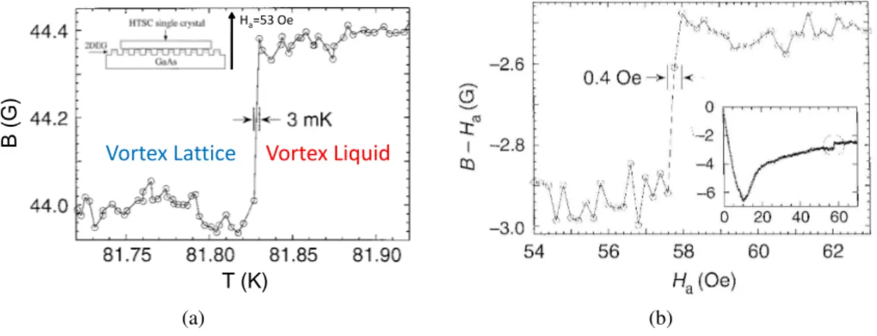
B ( G ) T (K) Ha=53 Oe Vortex Liquid Vortex Lattice (a) (b)

Figure 1.12: Vortex lattice melting observed through the local magnetic induction measurements. (a) Temperature scan: local magnetic flux density step at the first-order vortex-lattice melting (freezing) tran-sition in Bi2Sr2CaCu2O8measured with Hall sensor technique by decreasing the temperature at constant field of 53 Oe. The sample was cooled very slowly (5 ∼ 15 mK/min) (b) Field scan: local magnetic flux density step as the melting line is crossed by increasing the applied field at 80 K. Inset: the entire local magnetization curve (also called the self-field curve), B − Ha, as a function of increasing applied field Ha (Figures from [24]).

E. Zeldov et al. observe [24] that in swept field measurements (Figure 1.12 (b)), the

step occurs at the same value of the local induction Bz at various locations across the

sample, but at different values of Hext due to the non-uniformity of the Bz profile across

the sample.

As a result, in standard global magnetization measurement, the observed step is ac-tually an value averaged over the entire sample; the variation of the magnetic moment with external field is in general broader and smoother, masking the underlying physical phenomena [24].

The microscopic Hall probe sensors used in [24] have an active area of 3×3 µm2_and

the active layer of these sensors were located only ∼ 0.1 µm below the surface. There-fore a very accurate measurement of the local magnetic field with the spatial resolution corresponding to the size of the active area, 3 µm, was obtained.

(28)

1.6. Phase diagram for vortex system inBSCCOwith disorder and vortex shaking experiments27 lattice state (Figure 1.12). By temperature scans as shown in Figure 1.12 (a), one can

define the melting temperature Tm above which the magnetic induction (increasing) step

occurs; Similarly, by field scans as shown in Figure 1.12 (b), one can define the melting field Bmabove which the magnetic induction (increasing) step occurs. Plotting the

corre-sponding values of (Tm, Bm) on a T-B diagram, one obtains a line that separates the vortex

liquid state and vortex lattice state (Figure 1.13). This line is called the first-order melting (freezing) transition line.

vortex liquid state

vortex lattice state

Figure 1.13: Vortex liquid to lattice transition line in Bi2Sr2CaCu2O8as measured by field scans (°) and temperature scans (2). The solid line is a fit to Bm(T ) = B0(1 − T /Tc)α, where α = 1.55, B0= 990 G, and Tc= 94.2 K (Figure from [24]).

1.6 Phase diagram for vortex system in BSCCO with

dis-order and vortex shaking experiments

The phase diagram for Bi2Sr2CaCu2O8 is shown in Figure 1.14. On this phase diagram,

the blue line, which also corresponds to a first order transition and seems to the continua-tion of the melting transicontinua-tion at lower temperature, separates two phases: a rather weakly pinned vortex lattice at low fields, and a more strongly pinned vortex liquid or glass at high fields [26], [27].

At high temperatures, vortex system is influenced by thermal fluctuations and pin-ning by defects in the superconductor is relatively weak. When temperature is decreased, the defects begin to pin the vortices and therefore it is more and more difficult to reach thermodynamic equilibrium in the sense of achieving a ground state with lowest energy. Experiments with micro-Hall probe sensors performed by E. Zeldov et al. [24] on BSCCO showed that the local magnetic induction step at melting was no longer observed when the temperature was decreased below a certain value (38 K for their sample shown in

(29)

Figure 1.14:BSCCO phase diagram (Based on the phase diagram provided by E. Zeldov). Figure 1.15), called the critical point. If the same measurement is repeated in presence of an in-plane ac field, one finds a fully reversible magnetization and the self-field step characteristic for a first order transition can be once again observed [28] (Figure 1.16).

T = 38 K B ~ 400 G Critical point:

m m

Figure 1.15: Magnetization step, characteristic for a first order transition, was not any more observed be-low 38 K in BSCCO single crystals measured by E. Zeldov et al. (Figure from [24]).

-80 -60 -40 -20 0 20 0 100 200 300 400 500 H_a [ Oe ] with H_ac_⊥ without H_ac_⊥ T = 30 K B -Ha [ G ] 300 320 340 -28 -26 -24 Ha[ Oe ] T = 30 K < Tcp B -Ha [ G ] with H_ac_⊥

Figure 1.16:Magnetization loop with "vortex shak-ing". With the application of an in-plane ac field, the hysteresis is suppressed and the reversible magnetiza-tion step is observed (Figure based on slides provided by E. Zeldov).

Questions remain about the nature of the "shaken" equilibrium compared to a real thermodynamic equilibrium. As P. Gammel has pointed out, the unique properties of

(30)

1.7. Scope of this thesis 29 shaken equilibrium can lead to phase diagrams determined by the shaking itself, rather than by a thermodynamic variable such as temperature [29].

The existence of the "vortex glassy state" is not yet confirmed, i.e., whether the dashed depinning line is a vortex liquid to "vortex glass" phase transition or just a continuous variation of the vortex mobility. If one can probe the dynamics of the vortex motion near to the depinning line, one can thus obtain information on the nature of the vortex state in this region.

1.7 Scope of this thesis

Three different length scales can be defined in high-Tc superconductors:

1. Microscopic level: properties of single flux lines and interaction of individual flux lines with defects.

2. Mesoscopic level: length scales ≥ 1 µm, i.e., defined on length scales larger than the correlation length of collective behavior of vortices.

3. Macroscopic level: the entire superconductor.

It is extremely important to obtain experimental information on mesoscopic level in high-Tcsuperconductors since it is on this length scale that the distribution of critical currents is

defined [30]. Moreover, the macroscopic inhomogeneities can be revealed by observation on this level, which permits one to verify whether the intrinsic properties of material under study have been obtained [31].

In this thesis, two experimental techniques have been employed and combined. Chap-ter 2 is devoted to the magneto-optical imaging technique, which corresponds to mesoscopic-level observation on superconducting samples. Differential magneto-optical imaging with different kinds of modulation are discussed in this Chapter. Magneto-optical imaging has been used for sample selection, verification after irradiation experiments, characteriza-tion, and transport current visualization in this work.

Chapter 3 deals with the experimental aspects of transport measurements. A good quality of electrical contacts on single BSCCO crystals is essential for performing trans-port measurements. We used photolithography to achieve electrical contacts on the sur-face of the crystals. This permits us to visualize the transport current flow in our BSCCO samples.

Chapter 4 studies the field and current distribution for a superconductor in a NMR field configuration. Conclusions drawn from this chapter are useful to correctly interpret the NMR data on type-II superconductors.

Chapter 5 is the main part of this thesis. In order to investigate the mechanisms that govern the vanishing of linear resistance, we have measured the vortex shear viscosity

(31)

in a 20 µm-wide channel confined structure [32]. The vortex confinement effects among different kinds of confinements are compared. The heavily irradiated contact pads remote from the edges allow one to probe vortex bulk properties. The shear flow resistivity data are compared with two models describing vortex liquid-solid transitions: the two dimensional melting mediated by separation of dislocation pairs and the three dimensional Bose-glass transition.

(32)

Chapter 2 Magneto-optical imaging

In global magnetic measurements, one obtains an averaged value for the magnetic flux density over the entire sample. However, the physical phenomena under study are often masked or otherwise inaccessible because the averaging masks out small local changes of the flux density. A good example is the magnetization of a ferromagnet which contains the averaged information of flux density variations associated with the presence of magnetic domains. It is thus important to perform local magnetic field measurements. Magneto-optical imaging is a powerful tool since it permits one to obtain an image of the local magnetic flux density at the surface of the entire sample. The physical principe underlying magneto-optical imaging is the Faraday effect.

2.1 Faraday effect

The Faraday effect is a consequence of the fact that the magnetic field removes the sym-metry for the propagation of left-handed and right-handed circularly polarized light.

y y

E e

E =

E

VBL

F

=

θ

B

L

k

x

e

y

e

z

e

Figure 2.1:Linearly polarized incident light traverses the media (from the left to the right) in the presence of an axial magnetic field B (along the z-axis). k denotes the wave vector of the light. The electric field

vector E rotates an angle θF=VBL. This effect was discovered by M. Faraday (1791 - 1867) in 1845.

Linearly polarized light can be seen as a combination of a right circularly polarized 31

(33)

wave and a left circularly polarized wave with the same phase. When linearly polarized light propagates through certain media with different indices of refraction for waves of the two polarizations (right circular and left circular) in the presence of a magnetic field, at exit the right and left circularly polarized waves will have acquired different phases. The transmitted light at the exit is still linearly polarized but its electric field vector E has been

rotated over an angle θF which is proportional to the magnitude of the axial magnetic

field B and the length L that the light has traversed in the media: θF =

V

BL, where

V

is

called the Verdet constant, which is material and wavelength dependent.

There is a simple relation between the Verdet constant and the wavelength dependence of the index of refraction which was first derived by J. Larmor using a semi-classical calculation in 1898 [33]:

V

= − e

2mcλ

dn

dλ, (2.1)

where e is the charge of an electron, m is the mass of an electron, c is the speed of light, λ is the wavelength of light and n is the index of refraction of the medium. This relation works very well for gases, while for solids, one needs to add a dimensionless constant

C

to include the deviation of the Verdet constant from the value predicted by Equation (2.1):

V

= −

C

e

2mcλ

dn

dλ (2.2)

In cgs units, the Verdet constant has units of radians · Gauss−1_{· cm}−1_.

The Verdet constant for most materials is extremely small. For example,

V

= 3.80 ×

10−6radians · Gauss−1· cm−1for water at 20◦C and for light at 589 nm.

The Faraday effect can be used for magnetic measurements. As most of the supercon-ductors have very small Verdet constant, one places an "indicator film" which presents a high Verdet constant on the top surface of the superconductor in question. This indicator film detects the magnetic field at the surface of the superconductor. The Faraday active layer in the magneto-optical indicators that we use in our laboratory is a ferrimagnetic bismuth doped yttrium-iron garnet (Bi:YIG) layer.

Now we discuss the properties of magneto-optical indicators and the characteristics that we look for in a magneto-optical indicator.

2.2 Magneto-optical indicators

The YIG layers used in this work are a few microns thick. They are grown by liquid-phase epitaxy on a transparent gadolinium-gallium-garnet (GGG) substrate so that it can stand alone. To use it in a reflection mode, a very fine layer of Al, serving as a mirror, is evaporated on top of the YIG surface. The mirror is covered by a thin protective Ti-TiN layer and an anti-reflective layer is added to the substrate layer (Figure 2.2 (a)).

(34)

2.2. Magneto-optical indicators 33 The indicators that we use have a thickness of 4 µm for the YIG layer and a thickness of 0.5 mm for the substrate. Figure 2.2 (b) shows that a wafer of magneto-optical film was cut into different sizes adapted to samples of different dimensions.

(a) (b)

Figure 2.2: (a) Schematic representation for different layers in a magneto-optical indicator. (b) A wafer of magneto-optical indicators.

2.2.1 Magnetic properties of the layer Bi: YIG

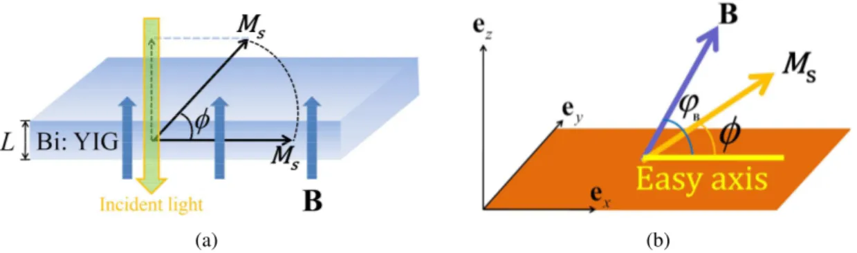
The MO indicator material is ferrimagnetic with a spontaneous magnetization, Ms, and

the easy axis lying in the film plane. A magnetic field B applied at an angle α (see Figure 2.3 (b)) will force the magnetization vector to turn out of the plane. We decompose B into the in-plane field component Bx and the out-of-plane field component Bz: Bx= BcosϕB,

Bz= BsinϕB. The Faraday rotation angle is given by: θF =

V

LMssinφ. There exists a

saturation rotation angle: θsat =

V

LMs. The presence of a parallel magnetic field yields

a reduced Faraday rotation angle θF. This behavior can be explained as follows.

(a) (b)

Figure 2.3: (a) The perpendicular magnetic field B induces the rotation of the magnetization vector Ms.

The perpendicular component of Msproduces the Faraday rotation. (b) The equilibrium tilt angle φ of the

magnetization Msis determined by the balance between the magneto-crystalline anisotropy of the Bi-YIG

(35)

Adopting the simplest form to find the equilibrium tilt angle φ, one minimizes the total magnetic energy composed of the anisotropy energy EA(1 −cos φ) and the dipolar energy:

E(B, φ) = EA(1 − cos φ) + BMs[1 − cos(ϕB− φ)].

The condition ∂E_∂φ = 0 yields:

tan φ = Bz

BA+ Bx,

where the anisotropy field BA≡ EA/Ms. As the Faraday rotation angle is proportional to

the component of Ms parallel to the propagation direction of the light (z-axis) it follows

that:

θF ∝ sin φ = p Bz

(BA+ Bx)2+ B2z

.

This model describes both the reduced Faraday rotation angle θF by a parallel field

and also the saturation for large Bz (sinφ → 1 for Bz À BA). Under normal operation

conditions for magneto-optical imaging, Bx is small and the Faraday rotation angle is

given by:

θF =

V

LMssinφ =

V

LMsq Bz

B2

A+ B2z

.

The relation between θF and Bz is approximately linear for a not too large value of Bz

(compared to BA defined by BA ≡ EA/Ms ∼ 600 - 1000 G, depending on the indicator

film):

θF = BzL

V

Ms

BA ≡ BzL

VMO

, (2.3)

where the Verdet constant for a MO indicator

VMO

is defined by:

VMO

=

V

Ms

BA =

V

M2

s

EA (2.4)

2.2.2 Doubled Faraday rotation to enhance the sensitivity

If, after passing through the magneto-optical layer, the light is reflected by a mirror and travels through the media again (the axial magnetic field is always present), the Faraday rotation will be doubled (Figure 2.4).

Denoting Iin as the incident light intensity, Ir as the reflected light intensity of the

magneto-optical indicator, of thickness L and absorption coefficient β (if one takes into account the optical absorption by the magneto-optical layer), one has: Ir = Iine−2βL. The

doubled Faraday rotation angle θ = 2θF, where θF=

V

MOBL. One defines a characteristic

constant k for an "indicator film" in reflection mode by: k ≡ θ/B = 2

V

MOL, k has the unit

(36)

2.3. Magneto-optical imaging 35

Figure 2.4:Faraday rotation doubled by a mirror. The Faraday rotation effect takes place at the Magneto-Optic Layer (MOL).

position to the polarization of the incident light. According to Malus’s law, the light intensity Iout behind the analyzer is then:

Iout = Irsin2(2

V

BL) = Iine−2βLsin2(2

VMO

BL). (2.5)

As one wishes to have a large signal Iout, Equation (2.5) shows that a magneto-optical

indicator should have a high Verdet constant and a low absorption coefficient.

If one takes into account the imperfection of the polarizer and the analyzer, the inten-sity measured once the light has passed the analyzer is: I = K0+ E₀2sin2θ, where θ = kB

is the Faraday rotation angle due to the presence of the magnetic field B, K0corresponds

to the background intensity, which describes the stray light and noise contribution to the signal, and E₀2≡ Iine−2βL. For a given indicator, β and L are constants, for convenience,

one uses E2

0, which has already taken into account the optical absorption by the

magneto-optical layer, to denote the incident light intensity. The polarizer and analyzer are usually not perfectly crossed, their relative angle is denoted as 90◦− α. The light intensity mea-sured after the analyzer is then:

I = K0+ E02sin2(θ + α). (2.6)

2.3 Magneto-optical imaging

The magneto-optical (MO) indicator is placed with the mirror side in contact with a flat sample (magnetic or superconductor, etc.). The linearly polarized light is incident on the indicator film from above, and is reflected from the aluminium layer placed in contact with the sample surface. While traveling in the indicator film, the light experiences a Faraday

(37)

rotation proportional to the perpendicular component of the local magnetic field. The lo-cal magnetic field information is obtained by observation through an analyzing polarizer, allowing one to detect the angle of Faraday rotation at each point on the sample surface. The image formed by the light, after it has passed through the analyzer is observed by an optical microscope (Figure 2.5 (a)). The intensity of the light is determined by the local perpendicular field Bz at the sample surface: bright regions in the magneto-optical image

corresponds to high Bz, while dark regions in the magneto-optical image corresponds to

low Bz(Figure 2.5 (b)).

(a) (b)

Figure 2.5: (a) Magneto-optic set-up for local magnetic flux density imaging at LSI (figure kindly pro-vided by Minoru Uehara, based on a photo of the real set-up at LSI). (b) Magneto-optical image formation: the contrast of the light intensity at the exit of the analyzer reflects the variation of the magnetic flux intensity of the surface covered by the MO indicator.

θ and α are usually less than 4◦_{, i.e., 0.07 in radian units, very small compared to π/2.}

Applying sin(x) ≈ x for x ¿ 1, one has1:

I = K0+ E02sin2(θ + α) ∼= K0+ E02(θ + α)2 (2.7)

1 _{In our study, we always work in this situation with magneto-optical imaging. The maximal value of}

the magnetic field generated by the coils that we use is about 400 Oe, this corresponds to a maximum rotation angle of 4◦_{(0.07 in radian units). The maximal difference between sin(x) and x in our study is thus}

(38)

2.3. Magneto-optical imaging 37

2.3.1 Magneto-optical indicators characterization: determination of

the absolute rotation angle

Equation (2.7) has three unknowns, K0, E₀2and θ. In order to recover the absolute value of

θ, one should perform three independent measurements of the intensity. For example, one chooses to measure at α = −α0, 0, and +α0(α0≈ 2◦), the corresponding light intensities

are denoted by I− , I0, and I+.

Using Equation (2.7), the Faraday rotation angle can be obtained by the following equation [34]:

θ = α0

2

I+− I−

I+− 2I0+ I− (2.8)

To perform this measurement, a Faraday active film (YIG garnet with perpendicular anisotropy) inserted in a copper coil is added in the optical path. The incident light ex-periences a Faraday rotation due to the nonzero magnetization of this YIG film when a current is applied to the coil. By changing the current, we modulate the angle α. We have used this method to characterize the magnetic response of our MO indicators.

-500 -250 0 250 500 - 6° - 4° - 2° 0 2° 4° 6° H_⊥_plane (Oe) Fa ra da y ro ta tio n an gl e:

θ _{measured Faraday rotation angle: θ}

(a) 0 50 100 150 200 250 300 1.0° 1.1° 1.2° 1.3° 1.4° 1.5° 1.6° T (K) Fa ra da y ro tat io n an gl e: θ

measured Faraday rotation angle: θ

(b)

Figure 2.6: Magneto-optical indicator film characterization on the indicator denoted as "VS-55-K". (a) Measured Faraday rotation angle as a function of the external field, perpendicular to the plane of the garnet film, at T = 315 K and with white light. The relation is approximately linear and the proportionality constant is about 0.01◦_{/Oe. (b) Measured Faraday rotation angle as a function of the temperature at H}

⊥plane= 90 Oe with green light (wavelength λ ≈ 530 nm) by using a filter equipped in the interior of the microscope.

The measurements demonstrate (Figure 2.6 (a)) that our magneto-optical indicators

present a significant Faraday rotation (1◦ per 100 Oe). The response of the indicators

is approximately linear with very weak magnetic hysteresis. The value of the saturation field is about 900 Oe.

The indicator was cooled to T = 20 K with the presence of a constant perpendicular field of 90 Oe and then the liquid helium flow was stopped. A temperature was read every

(39)

5 seconds and its corresponding rotation angle was measured during warm-up.

Figure 2.6 (b) shows that at low temperatures, our indicator presents a larger Faraday effect. This is consistent with the ferrimagnetic nature of the YIG layer: as the

sponta-neous magnetization Ms decreases when temperature is raised, one has a lower Verdet

constant

VMO

due to the Equation (2.4).

2.3.2 Optimization of image contrast

The field sensitivity of magneto-optical (MO) imaging is typically several Gauss. The non-uniform illumination, inhomogeneity of the MO indicator and dust presented on the optical path (dust on the indicator, infra-red filter, polarizers and other optical parts of the microscope) are the factors limiting the effective field resolution of the MO imaging technique.

Taking into account the imperfection of the analyzer, to optimize the image contrast, the analyzer and polarizer are set a little deviated from the crossed position. This angle was denoted as α in Equation (2.7).

E2

0 denotes the incident light intensity; T//and T⊥denote the transmittance of the light

polarized parallel and perpendicular to the transmission direction of the analyzer.

The light intensity received by the camera without (I1) and with (I2) application of the

magnetic field are:

I1= E02sin2α · T//+ E02cos2α · T⊥ (2.9)

I2= E02sin2(α + θ) · T//+ E02cos2(α + θ) · T⊥ (2.10)

Developing Equation (2.10) as the first order in θ, one gets:

I2= E02sin2α · T//+ θ · E02T//sin2α + E02cos2α · T⊥− θ · E02T⊥sin2α

We define a contrast parameter C = I2−I1

I1 and maximize it. Assuming

T⊥ T_// ¿ 1 and α, θ ¿ 1 yields Copt ≈ 2θ s T// T⊥ for αopt= q T⊥ T_//.

The value for polarizer extinction varies typically from 20 dB to 40 dB. We can thus estimate that the optimal deviation angle lies between 0.57◦_{∼ 5.7}◦_.

The above calculation was presented in [35]. In practice, we determine the deriva-tion angle α by the maximum contrast perceived by eye. The main reason is that we need to adjust the definition of the contrast parameter as a function of our experimental goal: revealing inhomogeneity and macroscopic defects (contrast between different re-gions within one sample), or the diamagnetic behavior revealed by the superconducting

(40)

2.4. Experimental setup for magneto-optics 39 sample as a whole (contrast between the sample and the background) in order to deter-mine, e.g., the critical temperature Tcor the critical current density jc.

2.4 Experimental setup for magneto-optics

The sample covered by the magneto-optical indicator is mounted in a special cryostat

(Oxford Instruments MicrostatHer) providing temperatures as low as 6 K with optical

access from above. The sample can be viewed through a window (it is also an infra-red filter in order to avoid the thermal radiation) in the cryostat and details of the magnetic flux distribution could be studied using a microscope with polarized light. Focusing and XY-translation are enabled by mounting the cryostat on an adjustable XYZ-stage.

The MO indicator and the sample are placed on a OFHC (Oxygen-Free High Conduc-tivity) copper sample holder, which is directly fixed to the cold finger of the flow cryostat. An indium foil is crushed between the sample holder and the cold finger in order to im-prove thermal contact. The whole mount is inserted into the cylindrical vacuum space.

A split coil copper magnet is mounted on the aluminium lids of the vacuum chamber. These coils are used for the application of a magnetic field component (up to 550 Oe) per-pendicular to the sample plane. In addition, one can also apply a magnetic field parallel to the sample plane by using another copper wire magnet. An iron core can be added into this wire magnet in order to strengthen the magnetic field. The whole setup is mounted on an optical table to minimize mechanical vibrations (Figure 2.7).

(a)

coils (perpendicular field) polarizer

sample

sample holder _cryostat

ocular analyzer C C D filters computer liquid helium MO indicator (garnet film) lamp objective (b) Figure 2.7:(a) Photo of the experimental set-up at LSI for magneto-optics. (b) Scheme of the experimen-tal setup.

(41)

(1) Cooling system and temperature control

A transfer line links a helium storage dewar to the cryostat. Liquid helium flows through the inner tube of this line to the heat exchanger of the cryostat. The returning helium gas flows along the outer tube of the line to the exhaust port. The exhaust line is linked to a helium gas flow controller and a small diaphragm pump. With the controlled

flow of helium, the MicrostatHer _{cools down quickly. The set-up permits us to reach a}

minimum temperature of 6 K. The temperature of the sample holder could be stabilized (variation ≤ 0.02 K) in a broad range (from 10 K to 500 K) using a temperature controller (Lakeshore 340). However, the liquid helium flow rate must be regulated by the experi-menter depending on the temperature range.

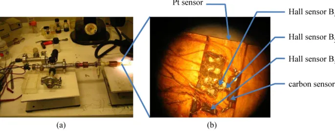
(2) Probes for measuring the temperature and the magnetic fields Pt sensor Hall sensor Bz Hall sensor By Hall sensor Bx carbon sensor (a) (b)

Figure 2.8:(a) Photo of the MicrostatHer_{. (b) Photo of the sample holder and placement of the sensors.}

The sensors are situated near to the sample, but in the opposite side of the sample holder.

Two temperature sensors (Pt-sensor and Allen-Bradley carbon sensor) were glued on the sample holder in order to measure the temperature. Three Hall probes are used for measuring the magnetic field components (Bx, By,Bz). These are positioned near to the

sample on the opposite side of the sample holder (see Photo 2.8 (b)).

The electrical access onto the MicrostatHer_{system (see Photo 2.8 (a)) is via a 10-pin}

connector and an additional 19-pin Amphenol connector. The connections (1, 2, 3, 4) are for carbon sensor, (5, 6, 7, 8) are for Schlumberger Hall probe to measure the Bzfield, (9,

10, 13, 14) and (11, 12, 13, 14) are for two Toshiba Hall probes to measure the Bx and

the Byfields. (15, 16, 17, 18) are reserved for 4-wire resistivity measurements. 19 is not

Heterogeneous vortex dynamics in high temperature superconductors

HAL Id: tel-00467466

https://pastel.archives-ouvertes.fr/tel-00467466

superconductors

Feng Yang

To cite this version:

Thèse pour obtenir le grade de

DOCTEUR DE L’ÉCOLE POLYTECHNIQUE

Specialité : Physique

par

Feng YANG

Heterogeneous vortex dynamics

in high temperature superconductors

Soutenue le 18 juin 2009 devant le jury composé de :

Thèse préparée au Laboratoire des Solides Irradiés,

Ecole Polytechnique, 91128 Palaiseau, France.

Remerciements

Contents

Chapter 1

Introduction

1.1 Superconductivity as a thermodynamic state

1.2 Magnetic properties for superconductors

1.2.1 Magnetization curves for type-I and type-II superconductors

1.2.2 Magnetic measurements

1.3 Vortex lattice

1.3.1 Surface barriers: the Bean-Livingston surface barrier and the

geometrical barrier

1.3.2 Vortex motion in type-II superconductors

1.3.3 Vortex pinning in type-II superconductors and irreversible

mag-netization

1.4 High-T

superconductors

s

d

1.5 Melting of the vortex lattice

1.6 Phase diagram for vortex system in BSCCO with

dis-order and vortex shaking experiments

1.7 Scope of this thesis

Chapter 2

Magneto-optical imaging

2.1 Faraday effect

E e

E =

E

VBL

=

θ

B

L

k

e

e

e

V

V

V

C

V

C

V

2.2 Magneto-optical indicators

2.2.1 Magnetic properties of the layer Bi: YIG

V

V

V

V

V

VMO

VMO

VMO

V

V

2.2.2 Doubled Faraday rotation to enhance the sensitivity

V

V

V

VMO

2.3 Magneto-optical imaging

2.3.1 Magneto-optical indicators characterization: determination of

the absolute rotation angle