HAL Id: tel-01191697
https://pastel.archives-ouvertes.fr/tel-01191697
Submitted on 2 Sep 2015
HAL is a multi-disciplinary open access archive for the deposit and dissemination of sci-entific research documents, whether they are pub-lished or not. The documents may come from teaching and research institutions in France or abroad, or from public or private research centers.
L’archive ouverte pluridisciplinaire HAL, est destinée au dépôt et à la diffusion de documents scientifiques de niveau recherche, publiés ou non, émanant des établissements d’enseignement et de recherche français ou étrangers, des laboratoires publics ou privés.
Adrien Le Guennec
To cite this version:
Adrien Le Guennec. Fast 2D NMR spectroscopy for complex mixtures. Chemical Sciences. Ecole Polytechnique, 2015. English. �tel-01191697�
École Doctorale de l'X
Spécialité Chimie analytique
Année 2015 N° :
Thèse
Pour l'obtention du grade de Docteur
par
Adrien Le Guennec
Titre de la thèse:
Fast 2D NMR spectroscopy for complex mixtures
Soutenance le 17 Juillet 2015
Composition du jury:
Mme Corinne GOSMINI Chercheur - Ecole Polytechnique, Palaiseau Présidente
M. Burkhard LUY Professeur - Karlsruhe Institute of Technology (KIT) Rapporteur
M. Nicolas GIRAUD Maître de Conférences - Université Paris-Sud Rapporteur
M. Dominique ROLIN Professeur - INRA/Université de Bordeaux Examinateur
M. Jean-Nicolas DUMEZ Chargé de recherche - ICSN, Gif-sur-Yvette Examinateur
M. Stefano CALDARELLI Professeur - ICSN, Gif-sur-Yvette Directeur de thèse
Contents
Remerciements ... 1
Notation and abbreviations ... 2
Introduction ... 7
Part 1. Literature survey ... 10
1. 1D NMR for metabolomics: principles and limitations ... 10
1.1. Metabolomics: goal and main tools ... 10
1.2. Metabolomics with 1D NMR ... 11
1.2.1. General considerations ... 11
1.2.2. Main statistical tools ... 12
1.3. Suppression of the solvent peak in 1D NMR of biological samples ... 13
1.4. Measurement of T1/T2 parameters ... 16
1.5. Limits of 1D 1H NMR for metabolomics ... 18
2. 2D NMR for complex-‐mixture analysis ... 20
2.1. Basics of 2D NMR ... 20
2.2. Basic 2D pulse sequences and important improvements ... 22
2.2.1. Homonuclear J-‐resolved spectroscopy (J-‐RES) ... 22
2.2.2. COrrelation SpectroscopY (COSY) ... 23
2.2.3. TOtal Correlation SpectroscopY (TOCSY) ... 25
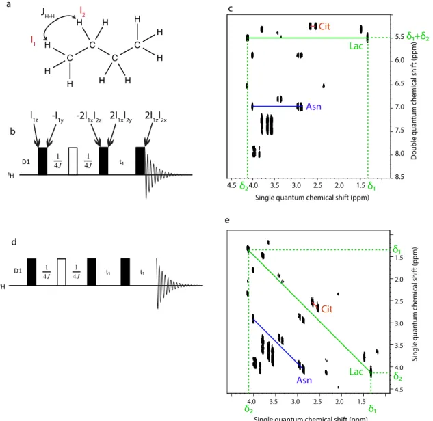
2.2.4. Double-‐quantum spectroscopy (DQS) ... 26
2.2.5. Heteronuclear Single-‐Quantum Coherence (HSQC) and Heteronuclear Multiple-‐Quantum Coherence (HMQC) ... 29
2.3. Previous studies in 2D NMR for quantification in complex mixtures and metabolomics 31 2.3.1. Quantification ... 31
2.3.2. Metabolomics ... 33
3. Strategies for the reduction of experimental times in multi-‐dimensional NMR ... 36
3.1. Reduction of the inter-‐scan delay ... 37
3.1.1. Band-‐Selective Optimized-‐Flip-‐Angle Short-‐Transient (SO-‐FAST) and Band-‐selective Excitation Short-‐Transient (BEST) ... 37
3.1.2. Acceleration by Sharing Adjacent Polarization (ASAP) ... 38
3.1.3. SMAll Repetition Times (SMART) NMR ... 39
3.2. Reduction of the number of t1 increments ... 39
3.2.1. Linear methods ... 39
3.2.1.1. Folding-‐aliasing ... 39
3.2.1.2. Linear prediction ... 40
3.2.1.3. Covariance NMR ... 41
3.2.2. Non-‐linear methods ... 41
3.2.2.1. Non-‐Uniform Sampling (NUS) ... 41
3.2.2.2. Radial sampling and projection-‐reconstruction ... 43
3.2.3.1. Hadamard spectroscopy ... 44
3.2.3.2. Ultrafast (UF) 2D NMR ... 44
3.2.4. Applications of fast 2D NMR approaches for complex mixtures ... 50
Part 2. Testing conventional 1D and 2D NMR experiments for metabolomics ... 52
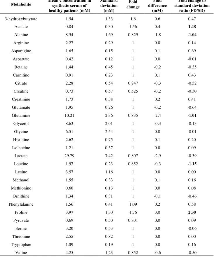
1. Preparation of synthetic samples relevant for metabolomics ... 52
1.1. Designing the synthetic samples for statistical analysis ... 52
1.2. Statistical analysis of the concentrations ... 53
2. One dimensional spectra, statistical analysis and limits of 1D NMR for metabolite identification ... 56
2.1. Acquisition parameters ... 56
2.2. Analysis of the 1D spectrum, discussions and conclusions for the composition of the synthetic serums ... 57
2.3. Bucketing and statistical analysis ... 58
3. Two dimensional spectra, statistical analysis and comparison of different pulse sequences ... 60
3.1. J-‐resolved pulse sequence ... 60
3.1.1. Parameters for acquisition and processing ... 60
3.1.2. Results and statistical analysis ... 61
3.2. COSY pulse sequence ... 63
3.2.1. Parameters for acquisition and processing ... 63
3.2.2. Results and discussion ... 63
3.2.3. Statistical analysis ... 64
3.3. HSQC pulse sequence ... 66
3.3.1. Parameters for acquisition and processing ... 66
3.3.2. Results and discussion ... 66
3.3.3. Statistical analysis ... 67
Part 3. Evaluation of fast 2D experiments for metabolomics ... 69
1. Calibration of fast 2D experiments for metabolomics analysis ... 69
1.1. Non-‐Uniform Sampling (NUS) ... 69
1.1.1. NUS DQF-‐COSY ... 70
1.1.1.1. Parameters for acquisition and processing ... 70
1.1.1.2. Results and discussion ... 70
1.1.2. NUS HSQC ... 71
1.1.2.1. Parameters for acquisition and processing ... 71
1.1.2.2. Results and discussion ... 72
1.2. UltraFast (UF) 2D NMR ... 72
1.2.1. UF COSY ... 73
1.2.1.1. Parameters for acquisition and processing ... 73
1.2.1.2. Results and discussion ... 74
1.2.2. UF J-‐RES ... 75
1.2.2.1. Parameters for acquisition and processing ... 75
1.2.2.2. Results and discussion ... 75
1.3. SOFAST/BEST: tests with inversion-‐recovery ... 76
1.3.1. Evaluation of the inversion-‐recuperation with selective pulses for T1 calculation ... 77
2. Statistical analysis and comparison between fast and conventional 2D NMR ... 79
2.1. NUS DQF-‐COSY ... 79
2.2. NUS HSQC ... 80
2.3. UF COSY ... 81
Part 4. Ultrafast double-‐quantum spectroscopy for diagonal-‐free 2D spectra ... 84
1. Development and optimization of the DQS pulse sequence ... 84
1.1. Calibrations of UF experiments for the 600 MHz ... 84
1.2. Development of the UF DQS pulse sequence ... 86
1.2.1. Behavior of double-‐quantum coherence during spatial encoding ... 86
1.2.2. Parameters for acquisition and processing ... 87
1.2.3. Results and discussion ... 88
2. COSY-‐like spectrum without diagonal peaks from the DQS pulse sequence ... 89
2.1. Processing approach to obtain a COSY-‐like spectrum from the DQS pulse sequence ... 89
2.2. DQS pulse sequence variant to obtain a COSY-‐like spectrum: symmetrized DQS pulse sequence ... 90
2.2.1. Description of the conventional and UF variants of the symmetrized DQS pulse sequences ... 90
2.2.2. Parameters for acquisition and processing ... 91
2.2.3. Results and discussion ... 91
3. Application of the UF DQS pulse sequence for the analysis of a complex mixture .. 93
3.1. Interleaved UF pulse sequences ... 93
3.2. Acquisition of UF DQS and UF DQSSY spectra in water and comparison with UF COSY 96 3.2.1. UF COSY and implementation of interleaved spectra ... 96
3.2.2. UF DQS ... 97
3.2.2.1. Parameters for acquisition and processing ... 97
3.2.2.2. Results and discussion ... 98
3.2.3. UF DQSSY ... 99
3.2.3.1. Parameters for acquisition and processing ... 99
3.2.3.2. Results and discussion ... 99
Part 5. Time-‐equivalent non-‐uniform sampling for complex-‐mixture analysis ... 102
1. Sensitivity-‐enhanced NUS for small molecules ... 102
1.1. Analysis of sensitivity in sensitivity-‐enhanced NUS ... 102
1.1.1. Parameters for acquisition and processing ... 102
1.1.2. Results and discussion ... 103
1.2. Accuracy of the volume reconstitution with the percentage of NUS ... 104
1.3. Role of the number of t1 increments for sensitivity in HSQC ... 106
2. Resolution-‐enhanced NUS for small molecules ... 107
2.1. Optimization of experimental conditions ... 107
2.1.1. Pulse sequences ... 107
2.1.2. Samples ... 109
2.1.3. Sampling schedules ... 109
2.1.4. Reconstruction algorithm ... 111
2.2. Analysis of sensitivity in resolution-‐enhanced NUS ... 112
2.2.2. Analysis of the HSQC and zf TOCSY spectra ... 114
2.2.2.1. Reconstruction fidelity and effect of resolution-‐enhanced NUS ... 114
2.2.2.2. Analysis of volumes ... 117
2.2.2.3. Analysis of noise ... 119
2.2.3. Analysis of peak intensity and S/N in resolution-‐enhanced NUS ... 120
2.2.3.1. Parameters for analysis ... 120
2.2.3.2. HSQC ... 121
2.2.3.3. zf TOCSY ... 122
Part 6. Estimation of T1 and T2 in complex mixtures ... 125
1. The T1 toolbox ... 125
1.1. The DOSY Toolbox ... 125
1.2. Equations for T1 measurements ... 129
1.3. First test: phenylalanine sample ... 129
1.4. The T1 Toolbox for T1 estimation of a complex mixture ... 130
2. IR pulse sequence with efficient solvent suppression ... 132
3. The T2 toolbox ... 135
3.1. Equations for T2 calculations ... 135
3.2. Use of CPMG with water suppression for T2 estimations ... 136
3.3. Evaluation of PROJECT for T2 estimation ... 137
Conclusion and perspectives ... 140
Tables and figures ... 142
List of publications and communications ... 156
Bibliography ... 157
Remerciements
Cette thèse a été effectuée au sein de l'équipe 64 du laboratoire de l'ICSN, à Gif-sur-Yvette, ainsi qu'à l'École Polytechnique de Palaiseau et le laboratoire CEISAM, à l'Université de Nantes. Je remercie le directeur de l'ICSN, Max Malacria, récemment remplacé par Angela Marinetti, ainsi que le chef de l'équipe du groupe RMN, Éric Guittet, pour m'avoir accueilli dans l'ICSN.
D'un point de vue professionnel, je souhaiterais remercier mes deux directeurs de thèse,
Stefano Caldarelli et Patrick Giraudeau, pour m'avoir donné ma chance pour cette thèse. Leur
disponibilité, même pour les détails les plus triviaux, a été très appréciée durant ces 3 années de thèse. Je voudrais également remercier d'anciens post-docs de Stefano Caldarelli; Robert Evans et
Manjunatha Reddy, qui m'ont également aidé durant le début de ma thèse afin de m'habituer à
certains paramètres de la RMN et de Topspin. Jean-Nicolas Dumez, qui est arrivé à l'ICSN au milieu de ma thèse, a été également d'une grande aide durant cette 2ème moitie de thèse.
Dans le laboratoire de l'ICSN, je souhaiterais également remercier tous les membres de l'équipe 64: Ewen Lescop, Nelly Morellet, François Bontems, Christina Sizun, Carine
Van-Heijenoort, Nadine Assrir, Éric Jaquet, Naima Nhiri Marion André, Yasmine Skanji, Gwladys Rivière, Arthur Besle, Séverine Moriau, Celia Deville, Safa Lassoued, Nelson Pereira, Ying-hui Yang, Oriane Frances, Prishila Ponien, Annie Moretto et Alda Da Costa,
avec qui j'ai pu avoir plusieurs conversations intéressantes qui m'ont aidé durant cette thèse, à la fois pour les recherches et pour la vie quotidienne du laboratoire.
Au laboratoire CEISAM, je remercie également tous les membres de l'équipe EBSI, tout particulièrement Illa Tea, qui a été respectivement encadrante et co-encadrante de mes deux premiers stages de laboratoire. Je souhaiterais également remercier Ingrid Antheaume, Benoît
Charrier, Virginie Silvestre, Denis Loquet, Estelle Martineau, Serge Akoka, Gérald Rémaud, Richard Robins, Meerakhan Pathan, Maxime Julien, Kévin Bayle, Ugo Bussy, François Kouamé, Didier Diomandé et Renaud Boisseau pour leur conseils et leur aide, que ce soit
durant les stages ou durant la thèse. Je souhaite également bonne chance à Boris Gouilleux et
Laetitia Rouger, qui entament leur thèse.
Je souhaiterais également remercier l'équipe 09 de l'ICSN, dirigée par Didier Stien et
Véronique Épervier, pour nous avoir laissé utiliser leurs laboratoire durant le déménagement du
groupe de Stefano Caldarelli de l'École Polytechnique vers l'ICSN, ainsi que Alain-Louis Joseph, de l'école Polytechnique, qui m'a également permis de mieux comprendre comment fonctionne la RMN.
D'un point de vue personnel, en plus de toutes les personnes cités précédemment, je souhaiterais également remercier ma famille, tout particulièrement ma mère Véronique, ma sœur
Julie et ma tante Corinne, qui m'ont permis de rendre ces 3 années de thèse agréables, que ce soit
Notation and abbreviations
1D One-dimensional
1
H Proton
2D Two-dimensional
ASAP Acceleration by Sharing Adjacent Polarization
B1 Radio-frequency pulses
BEST Band-selective Excitation Short-Transient
COSY COrrelation SpectroscopY
CPMG Carr-Purcell-Meiboom-Gill
CS Compressed Sensing
CV Coefficiant of Variation
CV-ANOVA Cross-Validated ANalysis Of VAriance
DANS Differential Analysis by 2D NMR Spectroscopy
DIPSI Decoupling In the Presence of Scalar Interactions
DNP Dynamic Nuclear Polarization
DISSECT DIagonal-Suppressed Spin-Echo Correlation specTroscopy
DOSY Diffusion Ordered Spectroscopy
DQ Double Quantum
DQF Double Quantum Filter
DQS Double Quantum Spectroscopy
DQSSY Double Quantum Spectroscopy SYmmetrized
DSE Double Spin Echo
ES Excitation Sculpting
FD/SD Fold Difference to Standard Deviation
FID Free Induction Decay
FT Fourier Transformation
GARP Globally optimized Alternating phase Rectangular Pulse
GUI Graphical User Interface
HMBC Heteronuclear Multiple-Bond Correlation
HMDB Human Metabolome DataBase
HMQC Heteronuclear Multiple-Quantum Correlation
HR-MAS High-Resolution Magic Angle Spinning
HSQC0 Time zero Heteronuclear Single-Quantum Correlation
IFT Inverse Fourier Transformation
ILT Inverse Laplace Transformation
IMPACT HMBC IMProved and Accelerated Constant-Time HMBC
INADEQUATE Incredible Natural Abundance DoublE QUAntum Transfer
Experiment
INEPT Insensitive Nuclei Enhanced by Polarization Transfer
IR Inversion Recovery J-RES J-RESolved JC-H Carbon-Proton J-coupling JH-H Proton-Proton J-coupling M3S Multi-Shot Single-Scan MaxQ Maximum-Quantum MDD Multi-Dimensional Decomposition MQ Multiple Quantum
MRI Magnetic Resonance Imaging
MRSI Magnetic Resonance Spectroscopic Imaging
NMR Nuclear Magnetic Resonance
NOE Nuclear Overhauser Effect
NOESY Nuclear Overhauser Effect Spectroscopy
NUS Non-Uniform Sampling
OPLS-DA Orthogonal Partial Least Squares-Differential Analysis
PCA Principal Component Analysis
PGFSE Pulse Gradient Field Spin Echo
PROJECT Periodic Refocusing Of J Evolution by Coherence Transfer
PURGE Presaturation Utilizing Relaxation Gradients and Echoes
Q-OCCA HSQC Quantitative, Offset-Compensated, CPMG adjusted HSQC
R2
Squared Pearson coefficient
SE Spin Echo
SEDUCE SElective Decoupling Using Crafted Excitation
SMART SMAll Recovery Times
SNR Signal-to-Noise Ratio
SNRmax Signal-to-maximum Noise Ratio
SO-FAST band-Selective Optimized Flip-Angle Short-Transient
SQ Single Quantum
T1 Longitudinal relaxation constant
T2 Transversal relaxation constant
T2*
Transversal relaxation constant with corrections for field inhomogeneities
TOCSY TOtal Correlation Spectroscopy
TPPI Time-Proportional Phase Incrementation
TR Repetition time
UF UltraFast
US Uniform sampling
UV Unit Variance
VIP Variable Importance for the Projection
WATERGATE WATER suppression by GrAdient-Tailored Excitation
WET Water Suppression Enhanced through T1 effects
zf z-filter
Introduction
Nuclear Magnetic Resonance (NMR) spectroscopy is one of the main analytical tools for metabolomics studies, along with mass spectroscopy, thanks to its high reproducibility and because it is a powerful tool to unambiguously identify metabolites.[1, 2]
NMR has become a common tool for metabolomics, thanks to a standardized strategy for sample preparation and analysis, based on
one-dimensional (1D) proton (1
H) spectra[3]
associated with statistical analysis.[4]
However, 1D 1
H spectra of complex mixtures, like biological extracts, are characterized by extensive overlap that can conceal part of the information from potential biomarkers.[5]
This extensive overlap also severely hinders absolute quantification, which is another important step for metabolomics studies.[6]
Alternative strategies have been used to limit the problem of overlap in 1D spectra. The use of other nuclei, like carbon-13 (13
C) have been shown to reduce greatly the problem of overlap, which gives an easier access to the information from most visible metabolites, as shown by the work from Wei et al.[7]
and Clendinen et al.[8]
, but this reduction of overlap comes at the price of the experimental time, since 13
C at natural abundance is far less sensitive compared to 1
H. Another possibility is the deconvolution of 1D 1
H spectra, initiated by the work from Weljie et al.,[9]
where the 1D spectrum is separated in different subspectra, each corresponding to the separate 1D spectrum of a metabolite,. But this analysis requires a good preliminary knowledge of the metabolites visible in the spectrum, in order to have a library of 1D spectra of individual metabolites recorded with conditions as close as possible to the conditions for the biological samples.
The last known possibility, which is explored in this thesis, is two-dimensional (2D) NMR. This technique, introduced in 1971 by Jeener[10]
and first applied in 1976 by Aue, Bartholdi and Ernst,[11]
makes it possible to spread peaks along two orthogonal frequency dimensions. Along with the lower risk of severe overlap, one of the most useful properties of 2D NMR is the added structural information, which makes this technique one of the cornerstones for structural elucidation. In addition, there is a great number of existing pulse sequences that allows the exploration of several types of connectivity, like J-couplings, Nuclear Overhauser Effects (NOE) or chemical exchange.
Since the introduction of NMR in metabolomics, several studies have been carried out to show the usefulness of 2D pulse sequences for metabolomics. Four pulse sequences in particular have been used for these studies. The first one is homonuclear J-RESolved (J-RES) spectroscopy, where J-couplings and chemical shifts are separated in two different dimensions. Since, in many cases, the overlap is caused by the J-couplings in 1D 1
H spectra, the separation makes it possible to reduce the overlap in the J-RES spectrum, even with biological samples.[12] The acquisition of
J-RES spectra has been optimized, by reducing the experimental time to levels close to 1D 1
H spectra with close sensitivity, in particular by the work of Viant and Ludwig.[13]
But the limited spectral width in the indirect dimension does not completely avoid the risk of overlap, artifacts from strong couplings can plague the J-RES spectrum[14]
and errors in quantification can arise because of partial cancellation.[15]
The Correlation SpectroscopY (COSY) and the TOtal Correlation SpectroscopY (TOCSY) pulse sequences are two others pulse sequences giving similar spectra, where connectivity between
protons is shown via J-couplings. But while COSY spectra show protons with direct J-couplings,[11]
TOCSY spectra show extended networks of J-couplings.[16]
So far, COSY in complex mixtures has been used in a recent strategy from the group of Schroeder at Cornell University, called Differentiation Analysis by Nuclear Spectroscopy, in order to discover more easily bioactive molecules in complex mixtures.[17]
For the TOCSY pulse sequence, a study by Van et al.[18]
has shown the potential of this pulse sequence to discover important metabolites by statistical analysis
that would be difficult to identify by 1D 1
H NMR. Band selective TOCSY has also been used for metabolomics studies[19]
and a variant has been used by the groups of Portais[20, 21]
and Markley[22]
to understand fluxes by 13
C enrichment. While these spectra usually have little overlap and are sensitive, one of their main shortcomings is the loss of information for some metabolites, particularly those without JH-H couplings.
Finally, the HSQC pulse sequence shows correlations between 1
H and 13
C (or 15
N,
depending on the system studied).[23]
This is one of the most used 2D pulse sequence for complex mixture analysis,[24-26]
since the 13
C dimension can give a higher spread of peaks and therefore reduces the risk of overlap. Studies by Simpson's group have also shown that 2D HSQC is a good
complement to 1D 1H spectra.[27-29] However, at natural abundance, HSQC is the less sensitive of
these four 2D pulse sequences but suffers from the low natural abundance of 13
C. This
disadvantage can however be decreased by 13
C enrichment, as long as it is commercially possible with the system under study, as shown for several studies by Kikuchi's group.[30, 31]
As seen from the description above, all the pulse sequences have strengths and weaknesses. But most of them share a similar problem: the experimental time for 2D spectra is much longer than 1D 1
H spectra because of the need to repeat hundreds of times the pulse sequence in order to construct the Free Induction Decay (FID) in the indirect dimension. In order to reduce the experimental time of 2D spectra, several approaches have been developed.
Two of them, in particular, have shown promises for reduction of 2D spectra of complex
mixtures. The first one is Non-Uniform Sampling (NUS), which can reduce the number of t1
increments by changing the method to acquire the indirect FID as well as the algorithm to reconstruct the 2D spectrum.[32]
Recent studies by Rai and Sinha,[33]
as well as Hyberts and al.,[34]
have shown that NUS can be used for complex mixtures to reduce the experimental times needed to record 2D spectra of complex mixtures, both for identification (with the use of very high resolution spectra) and quantification purposes (by reducing the acquisition time). The other
approach, called UltraFast (UF) 2D NMR, and proposed by Frydman and co-workers[35]
is the only current approach that makes it possible to record a 2D spectrum in only one scan.[36]
Despite compromises to make between spectral widths, resolution and sensitivity,[37]
improvements have made possible the quantification of metabolites in complex mixtures with concentrations as low as
At the beginning of this thesis, the pre-cited fast 2D NMR methods had not been evaluated for high-throughput metabolomics applications. Therefore, the goal of this thesis was to make a first evaluation of these fast 2D approaches for high-throughput metabolomics. In this manuscript, the main notions for the understanding of the subject will be introduced first, while the next chapters describe the strategies developed to reach this goal.
We made a first evaluation of these fast methods for untargeted metabolomics, using synthetic mixtures for metabolomics studies with 1D and 2D spectra. This study was separated in
two parts: the first part was focused on the differences between 1D 1
H spectra and conventional 2D spectra with three different pulse sequences (COSY, J-RES and HSQC) by using the statistical analysis of concentrations as a model. This study showed that the statistical analysis of 2D spectra was closer to the statistical analysis of concentrations than the statistical analysis of 1D spectra, confirming the usefulness of 2D spectra for metabolomics. Then the same comparison was made for conventional 2D NMR and fast 2D NMR, with the UF variant of COSY and the NUS variant of DQF-COSY and HSQC. These three variants were indeed compatible with metabolomics studies, since they made it possible to retrieve the same information as the conventional 2D counterparts, with a reduced experimental time.
Then, methodological developments were carried out in order to increase the amount of information available from fast 2D spectra. First, a new UF pulse sequence was developed based on double-quantum spectroscopy (DQS), in order to suppress diagonal peaks that can overlap with some correlation peaks. This sequence was tested with a sucrose sample and was compared to the UF COSY spectrum. Then another variant of UF DQS was tested to produce UF COSY-like spectra without diagonal peaks. And finally these two pulse sequences were tested with a sample of
several metabolites in H2O/D2O (90/10) to simulate biological extracts. A second optimization was
done with the NUS approach. The use of time-equivalent NUS was performed with its two variants, sensitivity-enhanced NUS and resolution-enhanced NUS. For resolution-enhanced NUS, an analytical evaluation was done to verify the sensitivity, the repeatability and the noise behavior, compared to conventional 2D NMR for two pulse sequences, HSQC and TOCSY. Finally, new tools were adapted for the measurement of T1 and T2, which are important parameters in NMR
since they impact the signal-to-noise ratio per unit of time. For that, a Diffusion-Ordered
SpectroscopY (DOSY) Toolbox was modified for the calculation of T1 and T2 and this toolbox was
tested for simple samples, followed by a complex mixture in H2O/D2O (90/10). For the last sample,
a solvent suppression scheme was tested for good water suppression without changing the accuracy of T1/T2 measurements.
Part 1. Literature survey
The goal of this chapter is to introduce the main concepts, which served as a basis for the present work. The limitations of 1D NMR for metabolomics are first discussed. The mechanism of several 2D pulse sequences and the resulting 2D spectra are then analyzed, in order to highlight their potential for metabolomics. Finally, the alternatives to conventional 2D acquisition are presented, with their pros and cons. Existing results of 2D NMR and fast 2D NMR for the analysis of complex mixtures will be also presented.
In this chapter, the general knowledge about multi-pulse 1D NMR will be assumed to be already known. This general knowledge includes the Zeeman effect, the effects of radiofrequency pulses on magnetization, the chemical shift, the J-coupling, nuclear spin relaxation, the vector model and the coherence transfer pathway model to explain the purpose of several pulse sequences and the effect of spin echo and INEPT building block on magnetization. For more details about these parts, the reader should refer to other references.[39, 40]
The use of product operators to explain the effect of two-dimensional (2D) pulse sequences is not indispensable, but can help to better understand the pulse sequences and their variants.
1. 1D NMR for metabolomics: principles and limitations
1.1. Metabolomics: goal and main tools
Metabolomics is a part of the 'omics analytical tools since at least 15 years, after the
sequencing of the human genome [41]
has shown its limits to fully understand the function of each gene.[42]
Its goal is the global understanding of the metabolome, i.e. the exhaustive list of small molecules participating in chemical reactions in an organism. Nowadays, metabolomics is considered one of the main branch of the 'omics family, along with genomics and transcriptomics, which studies DNA and RNA, respectively,[43] and proteomics, which focuses on proteins.[44]
Metabolomics has already shown to give complementary results to the other three 'omics techniques.[45]
While potentially every organism can be studied, the more common samples used are biofluids, like plasma, serum or urine,[46, 47]
and plants.[48, 49]
Because of the huge number of different chemical functions involved in organisms and the large dynamic range in concentrations, no analytical tool can achieve that goal with only one analysis. For that reason, metabolomics usually refers to any study where at least a subset of the metabolome is studied, for profiling or quantitative purposes.[6]
Despite this lack of universal analysis for metabolomics, two analytical tools are most commonly used today: NMR spectroscopy and mass spectrometry, the latter usually coupled to gas chromatography or liquid
chromatography.[50]
These two analytical tools are the closest universal detectors currently available within the analytical tools and gives reproducible results.
A classic metabolomics study consists of obtaining samples from several groups, for
example a control group and a diseased group in clinical research.[47]
between spectra from each sample should reveal metabolites that vary between groups, which should bring answers about metabolic pathways perturbed by the disease. Between these two analytical tools, mass spectrometry is generally considered as more sensitive, but the intensity of each peak is dependent on their ionization and behavior during chromatography, which makes quantification difficult. NMR, on the other hand, is less sensitive, but identification and quantification are easier.[51]
Finally, a sample used for mass spectrometry is destroyed, while a sample for NMR can be reused, for other NMR experiments or used for other analytical tools. Both are considered complementary techniques, with NMR for a good identification of the most abundant metabolites and mass spectrometry for detection of less concentrated metabolites.
1.2. Metabolomics with 1D NMR
1.2.1. General considerations
In most NMR studies for metabolomics, 1D proton (1
H) pulse sequences are used. The main reasons are the sensitivity of these spectra, the high reproducibility and because it is a primary analytical technique, which means that it is possible to measure the concentration from one experiment without the need of a calibration curve.[52, 53]
Its use for metabolomics requires several steps already described more than 10 years ago,[2]
and shown in figure 1.1.
Figure 1.1. The key stages of a NMR metabolomics study in order to obtain relevant biological
information. Reprinted with permission from A.C. Dona et al.[54]
Copyright 2014 American Chemical Society.
The reasoning behind these steps is to conserve all the biological information in the samples, by avoiding degradation of unstable metabolites or enzymatic activity and to limit fractionation by purification steps. Since one advantage of NMR is the possibility to analyze crude extracts without prior purification, the preparation of NMR samples are kept to a minimum, a part
that is standardized for some biofluids.[55]
The protocol for NMR experiments is also highly
standardized in order to harmonize results from several groups as much as possible.[3]
The extraction of intensities from the spectrum is done automatically by separating the spectrum into several regions, whose areas are used as the parameters for statistical analysis. The spectrum may be divided into regions of the same size, which is usually called binning, or regions of varying size depending on the peak size and overlap, which is usually called bucketing. However, the two terms can be used for either strategy in the literature.
While most of the steps stated above are automated, metabolomics studies are still dependent on the choice of the researcher. One of the most critical points in a metabolomics study is the sample collection. Since many factors influence the metabolome, like diet or age, the selection of patients for the study is important to limit as much as possible random modifications of metabolite concentrations between groups.[42, 56]
A critical analysis of results from statistical analysis is also required to avoid possible pitfalls.[57]
Two of the main pulse sequences used for metabolomics, 1D NOESY with water presaturation (noesypr1d) and excitation sculpting, only differ by their water suppression scheme. Indeed, the water suppression is critical in 1D 1
H spectra for metabolomics. The main water suppression schemes will be explained in the next section, including the two schemes stated above.
1.2.2. Main statistical tools
Because of the large amount of data generated by NMR spectra of biological samples, multivariate analysis is used to extract meaningful information about the system studied. A description of the different multivariate analyses is outside the scope of this review, but the basics of one of the most used multivariate analysis, principal component analysis (PCA) will be detailed below. Once raw intensities are extracted from the spectrum (for NMR or mass spectrometry), generally by fragmenting the spectrum into several regions, two questions are especially important. The first one is to know if the data allows a clear separation between groups and if it is the case, which part of spectrum contributes the most to the separation.
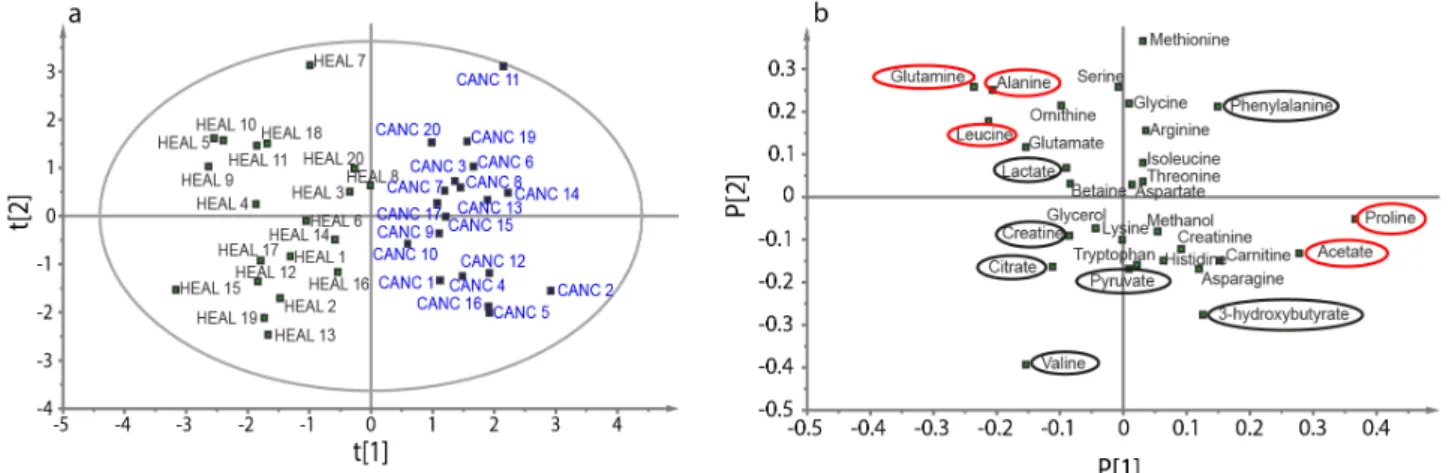
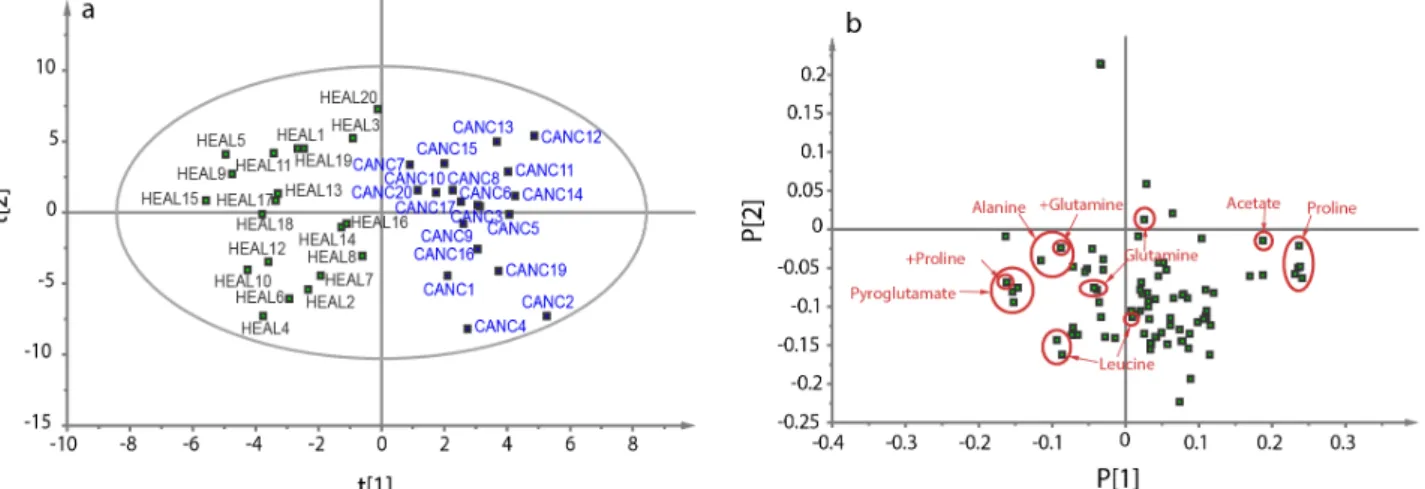
With PCA, the goal is to answer these two questions with a two-dimensional plot instead of the direct observation of all regions. From the intensity of each region, a new set of parameters is created, which are linear contributions of the intensities, as explained in figure 1.2.a.[4]
These parameters, called principal components, are created with the purpose of concentrating most of the total variance in the first new parameters. It is therefore possible to see most of the variance in a two-dimensional plot.
The first plot, called the score plot (figure 1.2.b), shows the position of each sample as a function of the two first principal components. It is a first start to see if the groups can be separated. The second plot (figure 1.1.c), called the loading plot, shows the coefficients of each region of the spectrum as a function of these two principal components. The bigger the coefficient, the more likely the region in question has an importance for the separation of the groups. The metabolites having the most importance in separation are the most likely to be important for the understanding of the system, and are often called biomarkers. Discovering these biomarkers is the
first step towards the understanding of the system studied and one of the main goals in metabolomics.
Other statistical tools exist to maximize the separation between groups, such as Orthogonal Partial Least Squares-Discriminant Analysis (OPLS-DA). This statistical tool is also a multivariate analysis, and produces the same plots as PCA. However, the separation involved directly the inter-group variability, instead of the total variance. This difference will be expended in part 2. Several tests also exist to verify the robustness of the results and their predictability, but are not within the scope of this review.
Figure 1.2. Scheme of principal component analysis (a), along with a scheme of the score plot (b)
and the loading plot (c). In the score plot, the ellipse represents the 95% tolerance for outliers based on the Hotelling distribution T2. Any point outside of this ellipse is a possible outlier,
whose profile is very different of the other samples and may be excluded from the analysis.
1.3. Suppression of the solvent peak in 1D NMR of biological samples
Most of the samples in NMR are in highly protonated water, usually a mixture of H2O/D2O
(90/10). A high concentration of salts is also typical, because of the biological sample itself or the use of a buffer to control the pH of the sample. This high concentration of protonated water will cause problems for NMR analysis if left unchecked, since 90% of protonated water means that the
sample has roughly 50 M of H2O, compared to the concentration of the metabolites, which is rarely
higher than tens of mM.[46] Another problem is the "faraway" water, which is the water at the edge
of the sample.[58]
Since this water does not exactly experience the same magnetic field as the rest of the sample, its chemical shift is slightly different and radiofrequency pulses do not have the same effect, creating a different coherence transfer than the rest of the signal.[59]
Finally, with these high concentrations, radiation damping can also occur,[60]
especially with cryogenic probes commonly used for NMR studies of biological samples.[61]
Radiation damping happens when the sample
S1 S2 S3 t1 X1 X2 X3 p2 Intensity X1’ X2’ X3’ X1’’ X2’’ X3’’ X3’’’ X2’’’ X1’’’ ... Sample S1 Sample S2 Sample S3
t1(S) = A1(X1) + A2(X2) + A3(X3) t2(S) = A2’(X1) + A2’(X2) + A3’(X3)
... p1 t2 t2(S2) t1(S2) A1 A1’ a b c Principal component analysis New parameters
magnetization (in this case, water magnetization) is coupled with the magnet magnetization, and acts as a selective pulse toward water, which returns the magnetization along the z-axis. In this case the water peak has a very short apparent T1, causing a very short T2* in the process and therefore a
large linewidth in the spectrum.[62]
These different problems cause different shortcomings, if left unattended. Because of the large dynamic range, problems can arise during the analog to digital conversion of the NMR signal to properly represent the peaks of the metabolites. It forces to choose low receiver gains to avoid artifacts, reducing sensitivity in the process.[63]
The combination of high concentrations with radiation damping means that most of the peaks in the spectrum will be altered by the water peak, by overlap or baseline distortion. The problem of "faraway" water will be important during the discussion on the different schemes to suppress water.
To avoid these problems, many schemes have been created to reduce as much as possible the water peak without altering the other peaks. The most used schemes for complex mixtures and diluted samples are represented in figure 1.3, along with two advanced schemes published recently that improve already existing schemes for cleaner spectra, especially for complex mixtures. All these schemes have pros and cons and no universal scheme exists, making each scheme more adapted for different cases, as explained in the next paragraphs.
Presaturation is one of the oldest solvent suppression schemes.[64]
It relies on the continuous irradiation of one frequency during the inter-scan delay to saturate the peak with this Larmor frequency, destroying its magnetization (figure 1.3.a). This simple scheme offers great reductions of the solvent intensity, but has three main problems: it can produce lineshape distortions, depending on the intensity of the residual peak;[53]
it works poorly on "faraway" water[59]
; it reduces
the intensity of protons in exchange with water, like the amide protons from proteins.[65]
However, a recent modification of this scheme is also effective against "faraway" water.[66]
The first increment of the Nuclear Overhauser Effect SpectroscopY (NOESY) pulse sequence with presaturation during the mixing time (noesy1Dpr, figure 1.3.b) has been developed in the case of metabolomics[67]
and has since then become one of the standard water suppression
scheme in metabolomics,[3]
since it requires little optimization.[68]
Compared to presaturation alone, noesy1Dpr benefits from a better volume selection and phase cycling, which allows a good suppression of "faraway" water.[69]
However, the scheme is sensitive to changes between samples (pH, salt concentrations...), which can cause different profiles for the water residual peak between samples.[70]
Water suppression Enhanced through T1 effects (WET) has been designed to be used in
localized NMR spectroscopy and imaging, where pulse power (B1) inhomogeneities and
longitudinal relaxation (T1) of water can lead to distortions in images and differences in water
suppression between spectra.[71]
This scheme uses selective pulses to put only the water magnetization in the transverse plane, which is then defocused by gradients. The robustness of
WET toward B1 and T1 effects comes from the difference in the tip angle for each selective pulse,
makes WET also adequate for liquid chromatography-NMR (LC-NMR), with the possibility to excite several frequencies simultaneously with one selective pulse.[72]
Since LC-NMR often uses mixtures of protonated solvents, several peaks have to be suppressed in order to identify peaks from other molecules. However, WET alone does not seem to be effective for 1D NMR in metabolomics, since the water residual peak is still important, with lineshape distortions and poor control of "faraway" water.[70]
Furthermore, it needs several optimizations (shape, spectral width and duration of the selective pulses) to eventually become efficient, which limits its use in metabolomics.
Figure 1.3. Basic solvent suppression schemes, with presaturation (a), first increment of the
NOESY pulse sequence with presaturation (b), WET (c), WATERGATE with selective pulses (d) or composite pulses (e) and excitation sculpting (f). Some advent solvent suppression schemes are
also shown, like PURGE (g) and "perfect echo" WATERGATE (h)
¹H Presat. D1 Grad ¹H ¹H ¹H ¹H ¹H ¹H ¹H D1 D1 D1 D1 D1 D1 D1 Grad Grad Grad Grad Grad Presat. Presat.
Pre. Pre. Pre. Pre. Pre. Pre. Pre.
b a c d e f g h 81.4° 101.4° 69.3° 161°
WATER suppression by GrAdient-Tailored Excitation (WATERGATE) are a series of schemes designed to change the relative angle of the water magnetization compared to those from other protons by the use of pulse field gradient spin echo (PFGSE), where an inversion is caused between two identical gradients. This can be achieved by selective pulses (figure 1.3.d)[73]
or composite pulses (figure 1.3.e).[74]
In both cases, the wanted coherence has been inverted, which allows it to be refocused by the last gradient, while the water peak experienced a 360° pulse as a whole, and thus is not refocused by the last gradient.
Since the water peak is not saturated, these schemes are adequate for protein NMR since they do not affect the signal of exchangeable protons. But the intensity of the nearby peaks is attenuated for each version, and the attenuation profile depends on the length of the selective pulses (selective WATERGATE) or the delay between pulses (composite WATERGATE). Furthermore, since the magnetization is inverted, WATERGATE is equivalent to a spin echo for this magnetization, causing the build up of anti-phase magnetization. Peak distortion is therefore found in the spectra, which can complicate the identification of the peaks in 1D spectra and limits its use for quantitative analysis. Baseline distortion due to the residual water peak also occurs, which can
be suppressed by a double PGFSE, also called Excitation Sculpting (ES, figure 1.3.f).[75]
While a shaped and a hard 180° pulses are used as a spin echo in this figure, any spin echo already used in WATERGATE can be used in ES. ES has been shown to give very reproducible water residual peaks and needs little optimization,[70]
which makes this scheme adequate for metabolomics.
Finally, two advanced water suppression techniques are also shown. Presaturation Using
Relaxation Gradients and Echoes (PURGE, figure 1.3.g)[76]
is an extension of the noesy1Dpr with a spin echo between the first and the second pulse and presaturation between delays. Gradients are also added during the mixing time and the scheme is repeated for better phase properties, similarly to double PGFSE. "Perfect" spin echo WATERGATE (figure 1.3.h) is an extension of ES where a
90° pulse is introduced between the two PGFSE.[77]
Any antiphase magnetization created during the first PGFSE is transferred by the 90° pulse and is reverted to in-phase magnetization by the second PGFSE, which is the mode of action for each "perfect" spin echo.[78]
It can also be added that
combination of schemes are possible, in order to suppress further the water peak.[59]
All these schemes are used in 1D 1
H spectra and can be integrated in two-dimensional pulse sequences or other multi-impulse pulse sequence.
1.4. Measurement of T1/T2 parameters
The longitudinal relaxation time (T1) and transverse relaxation time (T2) are two important
parameters in NMR that can be used to set the inter-scan delay and the acquisition time, respectively. The knowledge of the relaxation times can be used to optimize both parameters for optimal signal-to-noise ratio (SNR) per unit for time. The knowledge of T1 is also critical for
quantitative 1D NMR, since the area of a peak is dependent on T1 if complete relaxation has not
occurred between scans. A common value is five times the longest T1 to obtain an error of less than
For each relaxation time, several pulse sequences exist for its calculation. For T1, the main
pulse sequence is inversion-recovery (figure 1.4.a),[80]
where the magnetization is first inverted by a 180° pulse. A delay allows relaxation of the magnetization, then a 90° pulse is used to tip the magnetization in the transverse plane. By varying the delay between the 180° and the 90° pulse,
one can obtain a series of spectra with varying intensity depending on the T1 parameter. Another
possible pulse sequence is saturation-recovery. More details about T1 measurements will be shown
in part 6.
Figure 1.4. Pulse sequences commonly used for measurement of T1 and T2. Inversion-recovery
(a) is used for T1 measurement, while CPMG (b) is used for T2 measurement. Recently, the
PROJECT pulse sequence (c) has also been suggested for T2 measurements. Full rectangles are
90° pulses, while empty rectangles are 180° pulses.
For T2 measurements, the method of choice is the Carr-Purcell-Meiboom-Gill sequence
[81]
(CPMG, figure 1.4.b). After a 90° pulse, the magnetization undergoes several spin echoes. During
these spin echoes, the chemical shift does not evolve, but relaxation occurs depending on T2, more
precisely on T2*, which accounts for T2 as well as the effects of magnetic field inhomogeneity in
the sample. By varying the number of spin echoes, the resulting spectra have varying intensities
depending on T2*. More details about T2* measurements from these spectra will also be given in
part 6. D1 Variable delay
¹H
¹H
¹H
D1 D1 N N τ τ τ τ τ τa
b
c
Recently, a new pulse sequence has been reported for T2* measurements. This pulse
sequence is called Periodic Refocusing of J Evolution by Coherence Transfer (PROJECT).[82]
Like the "perfect echo" WATERGATE, the PROJECT uses "perfect" spin echo[78]
to avoid the presence
of anti-phase peaks in the spectrum, even with high delays between 180° pulses. A T2 analysis has
been recently published using this pulse sequence.[83]
Despite the existence of these pulse sequences, few studies in metabolomics or
complex-mixture analysis mention a study of T1 or T2 in order to set the acquisition delay or the
inter-scan delay,[84-86]
. Among the possible explanations for this low interest in T1 and T2 are the
highly congested 1D spectra of metabolomics mixtures, as detailed below, the fact that the
inter-scan delay and the acquisition delay is already suggested in the standard procedure,[3]
, that T1
and T2 are generally considered constants in all samples during one study, and therefore have no
impact for statistical analysis, or the lack of tools adapted for an automated measurement of the T1
and T2. More details about the last point will be given in part 6.
1.5. Limits of 1D 1
H NMR for metabolomics
While 1D 1
H spectra are the most sensitive spectra in NMR, the small spectral range of protons makes these spectra prone to peak overlap, especially in the case of complex mixtures, as shown in figure 1.5. While various degrees of complexity can arise from different biological media,[5, 46]
1D 1
H spectra are always characterized by a high degree of overlap between peaks. This overlap complicates the quantification of the metabolites, which is an important parameter for metabolomics.[6]
Figure 1.5. 1D 1H spectrum of a cell lysate. Reprinted with permission from K.Bingol and
R. Brüschweiller[5] Copyright 2014 American Chemical Society.
Even more importantly, this means that the regions delimited by spectral binning or bucketing can contain intensities from several peaks, and therefore several metabolites. This
complicates the statistical analysis and the identification of the biomarkers, since this brings uncertainty about the possible metabolites that are important for group separation. A more detailed explanation about the problems of peak overlap will be done in part 2.
Some methods to mitigate the problem of peak overlap have been developed in 1D spectra. The first is deconvolution of the 1D 1
H spectrum.[87]
It consists on the separation of the 1D spectrum into several subspectra of the different metabolites.[9]
This gives the possibility to quantify the metabolites and using directly the concentrations instead of peak intensities for statistical analysis. Since this method requires prior knowledge of the metabolites present in the mixture and focuses the study on these metabolites, deconvolution in metabolomics is often called metabolic profiling.
Despite this advantage, deconvolution has a few drawbacks, mainly the need for a library of the different metabolites to be quantified. Since the chemical shift of protons is sensitive to pH, salt concentration, magnetic field (for the chemical shift in Hz) and temperature, the library is also sensitive to these parameters. Also, since the peak intensity is dependent on acquisition and processing parameters, like acquisition time, inter-scan delay or the use of a window function (and therefore is similar to an external calibration),[52]
a good quantification of the metabolites needs to replicate correctly the acquisition parameters of the individual metabolites. One last limitation is the increased difficulty to correctly deconvolute the spectrum when peak overlap becomes more
preeminent, even with a good knowledge of the metabolites present in the mixture.[88]
For all these reasons, deconvolution mainly works for the simplest biological samples, with a good prior knowledge of the metabolite content and a standardized protocol for sample preparation and
spectrum acquisition, like plasma/serum[89]
and, to a lesser extent, urine.[90]
Another possibility is the use of other nuclei for NMR than 1
H. The main target for these studies is 13
C, thanks to its near-universal presence in metabolites, similarly to 1
H. By using 1D 13
C pulse sequences with 1
H decoupling during acquisition, it is possible to obtain spectra with high
spectral width (250 ppm instead of 10 ppm for 1
H) where every peak is a singlet.[91]
Peak overlap is therefore less important in 13C spectra compared to 1H spectra, while the direct proportionality
between peak area and concentration is the same as 1
H spectra. The increased resolution has proven to lead to better discrimination in multivariate analysis.[7, 8]
Plus, 13
C chemical shifts are less sensitive to pH and salt concentration than 1
H,[7]
making libraries of 13
C chemical shifts less sensitive on the medium studied.
However, this increased resolution comes with a reduced sensitivity, which arises from the
reduced gyromagnetic ratio (around 1/4th
of 1
H gyromagnetic ratio) and the low natural abundance of 13
C (around 1.1%). Because of this shortcoming, 13
C acquisition needs high concentrations or high acquisition times, which are not ideal for metabolomics. Another possibility is the use of microprobes optimized for 13
C direct dimension, which makes it possible to use less biological material in order to record a 13
C spectrum with acceptable experimental times for metabolomics.[92]
Isotopic enrichment is also possible to enhance sensitivity, but the peaks in the resulting 1D 13
C spectrum are not necessarily singlets anymore, because of the involvement of J-couplings between
13
C. 1
JC-C, in particular, is around 40-60 Hz, which increases the risk of overlap in 1D 13
C spectra.[5]
Other, more sensitive nuclei have been also used, like 19
F[93, 94]
or 31
P[95]
same success as 1
H or 13
C, as they are present only in a limited number of metabolites. Nevertheless, these nuclei can be useful for targeting groups of metabolites.
A last possibility, which will be discussed in the next section, is the use of multi-dimensional NMR, especially 2D NMR.
2. 2D NMR for complex-mixture analysis
2.1. Basics of 2D NMR
Two-dimensional (2D) NMR is a concept that has been developed in the seventies, which has revolutionized NMR, as explained below. It allows the acquisition of spectra with two frequency dimensions, with a wealth of different alternatives for these different frequencies. One of the biggest strength of 2D NMR is the possibility to directly see the connectivity between atoms, generally through bond or through space. This strength makes 2D NMR an important tool for the determination of molecular structure. Different 2D pulse sequences will be shown in later sections and will show at least a part of this wealth of information.
The general scheme for 2D NMR is shown in figure 1.6 and can be applied to describe almost any 2D pulse sequence with four subparts.
Figure 1.6. General scheme of a 2D pulse sequence.
The preparation aims to manipulate the magnetization in order to obtain the desired state for the evolution time. Generally, this subpart consists of the inter-scan delay and a 90° pulse to tip magnetization in the transverse plane, but more elaborate manipulations can occur for some pulse sequences.
The evolution is the first temporal dimension of the acquired FID. No acquisition is done during this time, but different scans with an incremented addition to this delay make it possible to obtain a FID, with each scan corresponding to a point in this FID, which are usually called t1
increments.
The mixing consists in further manipulations of the magnetization in order to obtain the desired state for acquisition. During this mixing, a transfer of magnetization is achieved, whose nature (coherence, polarization...) will be different for each pulse sequence.
) )
TR
NS
N
Finally, acquisition occurs, where a FID is recorded, similarly to 1D NMR. The time during which the probe records the signal is usually called t2.
The experimental time Texp of a 2D pulse sequence depends on 3 parameters: the time
necessary to complete the pulse sequence once, including the inter-scan delay, called the repetition time (TR), the number of scans (NS) necessary to complete phase cycling or for sensitivity issues
and the number of t1 increments (N1). Compared to 1D NMR, one new parameter is involved in the
calculation of Texp, which is N1. Since several points are needed to correctly represent the indirect
FID (usually several hundreds), the experimental time of 2D NMR is usually higher than 1D NMR for a similar sample, from several minutes to several hours for one spectrum. Each parameter has a minimum value: TR must be high enough to let enough magnetization return along the longitudinal axis between scans, for sensitivity issues as well as avoiding artifacts in certain cases, N1 is
dependent on the resolution needed in the indirect dimension and a minimal number of scans must be allowed for phase cycling, in order to suppress potential artifacts, or for sensitivity issues.
Once the bi-dimensional FID is acquired, Fourier transformation (FT) is used to obtain a 2D spectrum in the frequency domain. The strategy used in the FT algorithm in both dimensions is shown in figure 1.7, as used in most algorithms from commercial and public software.
Figure 1.7. Strategy to use Fourier transformation in a two dimensional FID, as treated by the FT
algorithm in commercial and public software.
From the 2D FID, which is stored as a matrix, FT is performed on one of the dimensions, in practice the direct dimension t2. In order to let the algorithm use FT in the second dimension, which
is the indirect dimension t1, the data matrix is then transposed. The 2D spectrum in the frequency
domain is then obtained. The F2 dimension is often referred as the direct dimension, since the FID
is directly recorded during acquisition, while F1 is the indirect dimension, since the FID is recorded
point by point with each t1 increment.
t1 t2 t1 F2 t1 F2 F1 F2 Fourier transformation along t2 Fourier transformation along t1
While phase-sensitive detection in the direct dimension uses the same strategy as 1D spectra, phasing in the indirect dimension requires other methods, by shifts in pulse phases between t1 increments (States,
[96]
Time-Proportional Phase Incrementation (TPPI)[97]
) or by changes in the sign of gradients (echo-antiecho[98]
). However, some 2D spectra are preferably displayed in magnitude mode, because of unfavorable phase properties. The content of a 2D spectrum will depend on the pulse sequence used to obtain the 2D FID. The next section will show some of the most used 2D pulse sequences, along with important improvements that have simplified the analysis of the spectra obtained from these pulse sequences.
2.2. Basic 2D pulse sequences and important improvements
For this section, only the pulse sequences used in later parts of the manuscript will be described. The spectrum shown for each pulse sequence has been acquired with a sample of 7 metabolites: lactate, alanine, asparagine, glycerol, serine, proline and citrate in H2O/D2O (90/10).
This sample will also be used in part 4. For COSY, TOCSY, DQS, HMQC and HSQC, the product operator formalism will be used for a better understanding of each pulse sequence. Unless specified, all the pulses are along the x-axis.
2.2.1. Homonuclear J-resolved spectroscopy (J-RES)
J-RES is one of the oldest 2D pulse sequence developed[99] and is not a correlation
experiment, but instead focuses on the separation of two parameters, the chemical shift and the J-coupling. The pulse sequence is shown in figure 1.8.a., which is one of the most simple 2D pulse sequences. After the 90° pulse, the evolution already starts, and a spin echo is used during the
evolution time in order to let only the J-couplings evolve during t1. No mixing is involved and the
acquisition starts immediately after evolution.
Figure 1.8. 2D pulse sequence for J-RES (a), along with J-RES DSE (b) and a J-RES DSE
spectrum of a mixture of 7 metabolites in H2O/D2O (90/10). All the pulses are along the x-axis.
During acquisition, both the chemical shifts and the J-couplings evolve, which means that the spectrum obtained immediately after FT does not directly separate the two parameters. Each
1.5 2.0 2.5 3.0 3.5 4.0 1H (ppm) -20 -15 -10 -5 20 15 10 5 0 nJ H-H (Hz) ¹H D1 ¹H D1 t /2 t /2 t /2 t /4 t /4 a c b
peak has the coordinates (δ+J; J) along F2 and F1, respectively, with δ representing the chemical
shift and J the J-couplings. In order to separate each parameter, an operation called tilting (also called shearing) can be used, which transforms each coordinate into a linear combination of these coordinates. For J-RES, each peak of coordinate (Ω1; Ω2) has the new coordinates (Ω1-Ω2; Ω2),
which finally gives the coordinates (δ; J) in the J-RES spectrum.[15]
The peaks have the desired coordinates, but are distorted,[13]
which can be resolved by symmetrization along F1 at the axis
J=0 Hz.
After this processing step, the J-RES spectrum is obtained, but this spectrum may contain artifacts from strong coupling.[14]
Since these artifacts undergo the same coherence pathway as the expected peaks, neither phase cycling nor gradients can be used to suppress them. However, this suppression can be obtained by a change in the pulse sequence and processing, with the J-RES Double Spin Echo (DSE),[14]
shown in figure 1.8.b. The main change between J-RES and J-RES DSE is a second 180° pulse that also acts as a spin echo. Since the genuine peaks and the artifacts have a different behavior during the second 180° pulse, it becomes possible to suppress the strong coupling artifacts by tilting and symmetrizing the spectrum.
The resulting spectrum can be seen in figure 1.8.c, and shows the complete separation of chemical shifts and J-couplings. This separation simplifies the analysis of the spectrum, especially in the region between 3.5 and 4 ppm. However, it also shows that the spectral width in the J-coupling dimension is small, not higher than 40 Hz, compared to several thousands of Hz in the chemical shift dimension. Therefore, this pulse sequence allows only a moderate increase in
resolution compared to 1D 1
H spectra.
A heteronuclear version of the J-RES pulse sequence has been developed shortly after the homonuclear variant,[100]
with the 1
H chemical shifts in the direct dimension and JC-H in the indirect
dimension. Contrary to homonuclear J-RES, the heteronuclear variant does not need shearing or symmetrization to completely separate the two parameters.
2.2.2. COrrelation SpectroscopY (COSY)
With J-RES, COSY is one of the first 2D pulse sequence developed.[11] Its purpose is to
show the direct neighbors of each proton through bond connectivity, in other words through J-couplings, as seen in figure 1.9.a. The pulse sequence, in its simplest form, is shown in figure 1.9.b. Only the magnetization from one spin I1 will be considered in the next paragraph, but the
analysis can be expended to the other proton spins of the molecule, like with the other pulse sequences presented in the next sections.
After the 90° pulse along x, which tilts the magnetization from I1z (longitudinal axis) to -I1y
(transverse plane), both the chemical shift and the J-couplings are evolving during t1. With these
evolutions, anti-phase magnetization 2I1xI2z is building up during t1, with I2 being another spin that
is sharing a J-coupling with I1. During the second 90° pulse, the anti-phase magnetization