HAL Id: hal-00865109
https://hal.inria.fr/hal-00865109
Submitted on 23 Sep 2013
HAL is a multi-disciplinary open access
archive for the deposit and dissemination of
sci-entific research documents, whether they are
pub-lished or not. The documents may come from
teaching and research institutions in France or
abroad, or from public or private research centers.
L’archive ouverte pluridisciplinaire HAL, est
destinée au dépôt et à la diffusion de documents
scientifiques de niveau recherche, publiés ou non,
émanant des établissements d’enseignement et de
recherche français ou étrangers, des laboratoires
publics ou privés.
Joint Power-Delay Minimization in Green Wireless
Access Networks
Farah Moety, Samer Lahoud, Kinda Khawam, Bernard Cousin
To cite this version:
Farah Moety, Samer Lahoud, Kinda Khawam, Bernard Cousin.
Joint Power-Delay
Minimiza-tion in Green Wireless Access Networks.
PIMRC 2013 - IEEE 24th International Symposium
on Personal, Indoor and Mobile Radio Communications, Sep 2013, London, United Kingdom.
�10.1109/PIMRC.2013.6666627�. �hal-00865109�
Joint Power-Delay Minimization in Green Wireless
Access Networks
Farah Moety
∗, Samer Lahoud
∗, Kinda Khawam
†, Bernard Cousin
∗∗University of Rennes I - IRISA, France †University of Versailles - PRISM, France
Abstract—Growing energy demands, the increasing depletion of traditional energy resources, together with the recent surge in mobile internet traffic, all call for green solutions to address the challenge of energy-efficient wireless access networks. In this paper, we consider possible power saving by reducing the number of active BSs and adjusting the transmit power of those that remain active while maintaining a satisfying service for all users in the network. We thus introduce a joint optimization problem that minimizes the network power consumption of the network and the sum of network user transmission delays. Our formulation allows us to investigate the tradeoff between power and delay by tuning the respective weighting factors. Moreover, to reduce the computational complexity of the optimal solution of our non-linear optimization problem, we convert it into a Mixed Integer Linear Programming (MILP) problem. We provide extensive simulations for various decision preferences such as power minimization, delay minimization and joint minimization of power and delay. The results we present show that we obtain power savings of up to 16% compared to legacy network models.
I. INTRODUCTION
Pushed by the needs to reduce energy, mobile operators are rethinking their network design for optimizing its energy efficiency and satisfying user Quality of Service (QoS) re-quirement
Currently, over 80% of the power in mobile telecommu-nications is consumed in the radio access network, more specifically at the base stations (BSs) level [10]. Thus, most of studies on energy efficiency in wireless network focus on the radio access. In the literature, various techniques are proposed for improving energy efficiency in wireless access networks such as decreasing the cell size, adapting power consumption to traffic load [3] or devising intelligent network deployment strategies using small, low power, femtocells and relays [10]-[12]. However satisfying user QoS has not been considered as a constraint in these works. Notable exceptions are the works in [8] and [11]. In [8], the authors proposed an optimization approach that minimizes power consumption in wireless access networks while ensuring coverage of active users and enough capacity for guaranteeing QoS. In [11], the authors formulated a cost minimization problem that allows for a flexible tradeoff between flow-level performance and energy consumption.
In this paper, we tackle the problem of power saving while minimizing the user delay in wireless access networks by finding a tradeoff between reducing the number of active BSs and adjusting the transmit power of those that remain active while maintaining a satisfying service for all users in the
network. Thus, we formulate an optimization problem that jointly minimizes the power consumption of the network and the sum of data unit transmission delays of all users in the network. Compared to prior works in the state of the art taking into consideration power saving and QoS, the optimization approach proposed in [8] does not support the feature of tuning the weights associated to the power and QoS cost; [11] uses an M/GI/1 queue for the delay model, which is a pessimistic bound compared to the realistic delay model we use in our paper. Moreover, [11] studies only the case where BSs switch between on and off modes without adjusting their transmit power.
We also tackle in this work the problem of user association: when an active BS is switched off or changes its transmit power level, users may need to change their associations. This coupling makes the problem more challenging. In our formulation, we consider the case of a Wireless Local Area Network (WLAN) using IEEE 802.11g technology. The design variable in this problem is to decide what follows:
• The running mode (on/off) of the network BSs and for active BSs, the corresponding transmit power level.
• The association of each user to which BS.
The key contributions of our work are as follows:
• We formulate the problem of power-delay minimization
in wireless access networks, going beyond the prior work in the literature which has focused either on minimizing energy without taking into consideration the QoS (i.e., delay) [10]-[3]-[12] or on delay analysis without taking into account energy minimization [9]-[7].
• Our problem formulation allows us to investigate the power-delay tradeoffs by tuning the weights associated to the total network cost components, namely power and delay.
• Starting from a non-linear formulation of the problem, we
provide a linearization process that makes the problem computationally tractable for realistic scenarios.
• The delay model provided in this paper is a unique feature
of our work, it is the realistic model used in IEEE 802.11 WLAN [6]-[9]-[7].
The rest of the paper is organized as follows. In Section II, we describe the system model considering an IEEE 802.11 WLAN. In Section III we present our proposed optimization approach and the linearization process. In Section IV we pro-vide extensive simulation results. Conclusions and perspectives
are given in Section V.
II. NEWORKMODEL
We consider the energy consumption of IEEE 802.11g WLAN, with Access Points (APs) working in infrastructure mode. We refer in the following to the term BS by the term AP as we consider the case of WLANs. As the downlink traffic on mobile networks is still today several orders higher than the uplink traffic, we only consider the downlink traffic (e.g., accessing web data) sent from AP to users. We assume that the network is in a static state where users are stationary. In other words, we take a snapshot of a dynamic system and optimize its current state. Furthermore, we assume that the network is in a saturation state, which means that we treat a worst case scenario where every user has persistent traffic. Moreover, when the AP is switched on, it is able to transmit at different power levels. We denote byNapandNlthe number
of APs in the network and the number of transmit power levels respectively. The indexes i ∈ I = 1, ..., Nap, and j ∈ J =
1, ..., Nl, are used throughout the paper to designate a given
AP and its transmit power level respectively. Note that, for j = 1 we consider that the AP transmits at the highest power level and for j = Nl the AP is switched off. We term by
k ∈ K = 1, ..., Nu, the index of a given user whereNu is the
number of users in the network.
A. Power Consumption Model
Adopting the proposed model in [10], the power consump-tion of an AP is modeled as a linear funcconsump-tion of average transmit power per site as below:
pi,j= L · (aπj+ b) (1)
wherepi,jandπj denote the average consumed power per AP
i and the transmit power at level j respectively. The coefficient a accounts for the power consumption that scales with the transmit power due to radio frequency amplifier and feeder losses while b models the power consumed independently of the transmit power due to signal processing and site cooling. L reflects the activity level of the APs. As we assume that the network is in a saturation state, L is equal to one, e.g., each active AP has at least one mobile requesting data with all resources allocated.
The cell coverage area in a cellular system is defined as the expected percentage of area within a cell that receives power above a given minimum. The transmit power at the AP is designed for an average received power at the cell boundary [4]. Thus, transmitting at different power levels leads to different coverage area sizes. Note that, all users within a cell require some minimum received Signal to Noise Ratio (SNR) for acceptable performance. Thus, in our paper, a user is considered covered by an AP if his SNR is above a given threshold.
B. Delay Model
We adopt the delay model presented in [6] and validated in our previous works [9]-[7]. We denote by χi,j,k the peak
rate perceived by user k from AP i transmitting at level j. Thus, when userk is associated to AP i transmitting at level j, his mean perceived throughput is given by [7]: Ri,j,k =
1/( 1 χi,j,k+
PNu k′=1,k′6=k
θi,k′
χi,j,k′), whereθi,k′ is a binary variable
that indicates whether userk′is associated to APi or not. We
denote byTi,j,k the amount of time necessary to send a data
unit to userk from AP i transmitting at level j. In fact, the delay needed to transmit a bit for a given user is the inverse of the throughput perceived by this user. Thus,
Ti,j,k= 1 χi,j,k + Nu X k′=1,k′6=k θi,k′ χi,j,k′ . (2)
Note that this model can be easily adapted to other wireless technologies such as 2G, WiMAX, or LTE systems [7].
III. OPTIMIZATIONPROBLEM
A. Problem Formulation
Our approach can be formulated as an optimization problem (P) that consists in minimizing the power consumption of the network and the sum of the data unit transmission delays of all active users.
We define the total network power and the total network delay as follows: the total network power is defined as the total power consumption of active APs in the network. The power consumption of an active AP, given in Equation 1, is modeled as a linear function of the average transmit power. Let λi,jbe a binary variable that indicates whether APi transmits
at level j or not. Thus, the total network power, denoted by Cp(λi,j), is given by:
Cp(λi,j) = X i∈I pi(λi,j) = X i∈I,j∈J pi,j· λi,j = X i∈I,j∈J (aπj+ b) · λi,j (3)
The total network delay is defined as the sum of data unit transmission delays of all users in the network. The data unit transmission delay Ti,j,k of user k associated to AP i
transmitting at level j is given in Equation 2. This delay depends on the transmit power of the AP the user is associated to. Recall that the binary variableθi,kindicates whether a user
k is associated to AP i or not. Thus, the total network delay, denoted by Cd(θi,k, λi,j), is given by:
Cd(λi,j, θi,k) = X i∈I,k∈K Tk(λi,j) · θi,k = X i∈I,j∈J,k∈K
Ti,j,k· λi,j· θi,k
(4)
Consequently, the total network cost, denoted by Ct(θi,k, λi,j), is defined as the weighted sum of power
and delay components and is given by the following: Ct(λi,j, θi,k) = αCp(λi,j) + ββ′Cd(θi,k, λi,j) (5)
β′ is a normalization factor and α and β are the weighting
factors that tune the tradeoff between the two components of the total network cost. Note that α + β = 1 and that α and
β ∈ [0,1]. In particular, when α equals 1 and β equals 0, we only focus on the power saving, and as α decreases and β increases more emphasis is put on the delay component.
Our problem(P) consists in finding an optimal set of active APs transmitting at a specific power level and an optimal user association that minimize the total network costCt(λi,j, θi,k).
Therefore (P) is given by:
MinCt(λi,j, θi,k) = α
X i∈I,j∈J (aπj+ b) · λi,j + ββ′ X i∈I,j∈J,k∈K (λi,j· θi,k χi,j,k + X k′∈K,k′6=k
λi,j· θi,k· θi,k′
χi,j,k′ ) (6) Subject to: X j∈J λi,j = 1 ∀i ∈ I (7) X i∈I θi,k= 1 ∀k ∈ K (8)
λi,j· θi,k= 0 ∀(i, j, k) : i ∈ I, j = Nl, k ∈ K (9)
λi,j ∈ {0, 1} ∀(i, j) : i ∈ I, j ∈ J (10)
θi,k∈ {0, 1} ∀(i, k) : i ∈ I, k ∈ K (11)
The objective function (6) provides the total cost of the network in terms of power and delay. Constraints (7) ensure that a given user is connected to only one AP. Constraints (8) state that every AP transmits only at one power level. In practice, when turning off some APs to accomplish power saving, some users will be uncovered. Thus, in our problem, to prevent users to be associated to a switched off AP, we add constraints (9). These equations ensure that λi,Nlandθi,k are
not both equal one. Indeed, when AP i is switched off, λi,Nl
is equal to one, then θi,k of all users cannot be equal to one.
Constraints (10) and (11) are the integrality constraints for the decision variablesλi,j andθi,k.
Moreover, to eliminate some trivial cases that are not included in the solution, we add the following constraints:
• If user k is not covered by AP i transmitting at the first
(highest) power level, then:
θi,k= 0 (12)
The equalities (12) prevent a given user to be associated to an AP if that user is not in the AP first power level coverage area.
• If user k is not covered by AP i transmitting at power level j, j ∈ {2, .., Nl− 1}, then:
λi,j· θi,k= 0 ∀j ∈ {2, .., Nl− 1} (13)
The equalities (13) ensure thatλi,j andθi,k are not both
equal one, and this prevents a given user to be associated to an AP if that user is not in the AP jth
power level coverage area.
Hence, solving problem (P) gives:
• The running mode of each AP and its corresponding transmit power. This is designated by λi,j for eachi ∈ I
andj ∈ J.
• The users association designated by θi,k for each i ∈ I
andk ∈ K.
B. Linearization Process
To reduce the complexity of our non-linear optimization problem (P), we convert it into a Mixed Integer Linear Programming (MILP). Thus, we replace the non-linear terms by new variables and additional inequality constraints, which ensure that new variables behave according to the non-linear terms they are replacing. Particularly, in the objective function (Equation 6) and in the constraints (9) and (13), we replace each quadratic termλi,j·θi,kby a new linear variableyi,j,kand
add the following three inequalities to the set of constraints: yi,j,k− λi,j≤ 0 ∀(i, j, k) : i ∈ I, j ∈ J, k ∈ K (14)
yi,j,k− θi,k≤ 0 ∀(i, j, k) : i ∈ I, j ∈ J, k ∈ K (15)
λi,j+ θi,k− yi,j,k≤ 1 ∀(i, j, k) : i ∈ I, j ∈ J, k ∈ K (16)
The inequalities (14) and (15) ensure that yi,j,k equals zero
when either λi,j or θi,k equals zero, while the inequalities
(16) force yi,j,k to be equal to one if both λi,j and θi,k
equal one. Moreover, constraints (9) and (13) will be replaced respectively by (17) and (18):
yi,j,k= 0 ∀(i, j, k) : i ∈ I, j = Nl, k ∈ K (17)
yi,j,k= 0 ∀j ∈ {2, .., Nl− 1} (18)
Similarly, we replace in the objective function (Equation 6) each quadratic termλi,j· θi,k· θi,k′ by a new variablezi,j,k,k′
and add the following inequalities to the set of constraints: zi,j,k,k′− λi,j≤ 0 ∀(i, j, k, k′) : i ∈ I, j ∈ J, k < k′ ∈ K
(19) zi,j,k,k′− θi,k ≤ 0 ∀(i, j, k, k′) : i ∈ I, j ∈ J, k < k′∈ K
(20) zi,j,k,k′− θi,k′ ≤ 0 ∀(i, j, k, k′) : i ∈ I, j ∈ J, k < k′∈ K
(21) λi,j+ θi,k+ θi,k′− zi,j,k,k′ ≤ 2 ∀(i, j, k, k′) : i ∈ I, j ∈ J,
k < k′ ∈ K (22) zi,j,k,k′− zi,j,k′,k= 0 ∀(i, j, k, k′) : i ∈ I, j ∈ J, k < k′ ∈ K
(23) The inequalities (19), (20) and (21) ensure thatzi,j,k,k′ is equal
to zero when eitherλi,j orθi,k orθi,k′ equals zero, while the
inequalities (22) force yi,j,k to be equal to one if λi,j, θi,k
andθi,k′ are equal to one. Furthermore, asλi,j· θi,k· θi,k′ =
λi,j· θi,k′ · θi,k, constraints (23) forcezi,j,k,k′ to be equal to
zi,j,k′,k.
In addition, we give the bound constraints for the variables yi,j,kandzi,j,k,k′which are introduced during the linearization
process:
0 ≤ yi,j,k≤ 1 ∀(i, j, k) : i ∈ I, j ∈ J, k ∈ K (24)
0 ≤ zi,j,k,k′ ≤ 1 ∀(i, j, k, k′) : i ∈ I, j ∈ J, k < k′ ∈ K
Notation Definition
Nap The number of APs
Nl The number of transmit power levels
Nu The number of users
pi,j The average consumed power per AP i
transmitting at power level j
πj The transmit power at level j
χi,j,k The peak rate perceived by user k
from AP i transmitting at level j
Ti,j,k The amount of time necessary to send a data unit to user k
from AP i transmitting at level j
θi,k A binary variable that indicates whether user k
is connected to AP i
λi,j A binary variable that indicates whether an AP i
transmits at power level j
yi,j,k A binary variable that indicates whether user k is associated
to AP i transmitting at power level j
zi,j,k,k′ A binary variable that indicates whether user k and user k′
are associated to AP i transmitting at power level j Table I
NOTATIONSUMMARY
Finally, our MILP problem (P′) is given by:
Min Ct(λi,j, yi,j,k, zi,j,k,k′) = α
X i∈I,j∈J (aπj+ b) · λi,j + ββ′ X i∈I,j∈J,k∈K (yi,j,k χi,j,k + X k′∈K,k′6=k zi,j,k,k′ χi,j,k′ ) (26)
Subject to the constraints:
(7), (8), (10), (11), (12) and (14) to (25).
The main notations used in our paper are reported in Table I. IV. PERFORMANCEEVALUATION
A. Evaluation Methodology
To evaluate the tradeoff between power and delay, we compute the optimal solution of our ILP using GLPK (GNU Linear Programming Kit) solver over a network topology composed of twelve cells (Nap= 9) covered by IEEE 802.11g
technology and six users in each cell (Nu= 9 ∗ 6 = 54). The
positioning of the WLAN APs in the network is performed following a grid structure and the positioning of users is generated randomly following a uniform distribution.
For the APs power model, we set for simplicity the number of transmit power levels to three (Nl=3). Indeed, in this
paper, we aim at computing the optimal solution of the MILP problem thus if we increase Nl, the granularity will be
finer but the problem will be intractable. We note that when j = Nl = 3, the AP is switched off, whereas an active AP
is able to transmit at two different power levels. The input parameters of the power consumption model in Equation 1 are given below:
• a = 3.2, b = 10.2 [12]
• π1 = 0.03 W and π2 = 0.015 W [2] are the transmit
powers when the AP is running on the first and the second power levels respectively.
Hence, the average consumed power per AP i at the first and the second power levels are given respectively by pi,1
= 10.296 W andpi,2= 10.248 W (i = 1, ..., 9). As mentioned
earlier, we assume that for j = Nl = 3, the AP is switched
off and therebypi,3= 0.
In addition, the coverage radius for the first and the second power levels are respectivelyR1 = 107,4 m andR2 = 75,8 m.
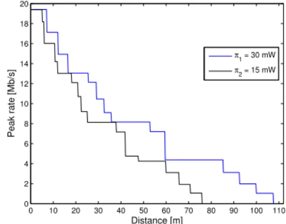
We obtain these values by simulation on Network Simulator (NS2) for a SNR threshold equals to -0.5 dB at the cell boundary. This SNR is the minimum value to be maintained in order to consider that a given user is covered by the AP. It corresponds to a cell boundary peak rate that equals 1 Mb/s in the downlink. Precisely, we implement in NS2 a benchmark scenario consisting of a free propagation model to characterize the WLAN radio environment, an IEEE 8021.11g AP working on 2.462 GHz (channel 11) and a single user at different positions. This user is receiving from the AP a Constant Bit Rate (CBR) traffic with a packet size of 1000 bytes and an inter-arrival time of 0.4 ms corresponding to a rate of 20 Mb/s. This leads to saturation state of the network according to the assumption presented in section II. In these conditions, the throughput experienced by our single user is the maximum achievable throughput (peak rate) for the current SNR. We run this scenario for each transmit power level of the AP (π1
= 0.03 W andπ2= 0.015 W) to obtain respectivelyχi,1,kand
χi,2,k for the corresponding user. When the average peak rate
of the user is equal to 1 Mb/s (target peak rate at the cell edge), we note the distance between the user and the AP for the two power levels and thus we obtain the corresponding radiusR1andR2. Figure 1 shows the peak rate perceived by
the user from the AP, transmitting at the first and the second power level, as a function of the distance between them.
0 10 20 30 40 50 60 70 80 90 100 110 0 2 4 6 8 10 12 14 16 18 20 Distance [m] Peak rate [Mb/s] π 1 = 30 mW π 2 = 15 mW
Figure 1. Peak rates in IEEE 802.11g for different transmit power levels.
To ensure the wireless signal reception by all users in the network, we generate their positioning in such a way each user is covered by at least one AP when all APs transmit at the highest power level. Figure 2 shows an example of our network topology where the distance between the APs is 120.8 m. With this distance, we obtain a dense coverage area where the average number of wireless signal layers is 2.02 (Table II). Table II shows the average number of wireless signal layers as a function of the distance (D) between the APs. In other words, it reflects, for each user, the average of number of covering APs (transmittting at the highest power level) with different inter-cell distances.D varies from (R1 +
Inter-cell distance [m] 120.8 134.2 147.6 161.1 174.5 187.9 201.3 214.8
Average number of wireless signal layers 2.02 1.76 1.53 1.38 1.25 1.15 1.05 1.00
Table II
WIRELESS SIGNAL LAYERSVSINTER-CELL DISTANCE.
AP First power level coverage
Second power level coverage
User
Figure 2. Network topology with inter-cell distance D = 120.8 m.
= 13.425 m. As D increases, the average number of wireless signal layers decreases as low as one when there is no overlap between the cells (D = 2R1).
Toward studying the tradeoff between minimizing the power consumption of the network and minimizing the sum of users delay in the network, we tune the values of the weightsα and β associated to power and delay components respectively, and investigate the obtained solutions. We consider three settings: the two weights are equal,α is very large compared to β and β is very large compared to α. Practically, the first setting, named Power-Delay-Min, matches the case where the power and delay components of the total network cost are equally important. The second setting, named Power-Min, matches the case where more preference is given to power saving. On the opposite, the third setting, named Delay-Min, matches the case where more importance is given to minimize the delay.
We compare the performance of our MILP solution for the considered settings with reference models for power and user association. The reference power model is denoted by the Highest Power Level (HPL) model as it assumes that all the APs transmit at the highest power level (j = 1). Under these circumstances, we consider a Power-Based user association (PB-UA) model. PB-UA model takes into consideration the power of the received signal at the user side in such a way the user connects to the AP where it gets the highest SNR. Afterward, the delay is calculated using Equation 2 according to the PB-UA model. These reference models are similar to the most frequently deployed WLAN networks, where APs transmit at a fixed transmit power level and users connect to the AP where they get the highest received signal strength [1]. Note that all results are the mean over 50 simulations with 95% confidence interval. Moreover, the normalization factor β′ is calculated in each simulation in such a way to scale the
two components of the total network cost [5]. Further, our MILP problem is solved using a linear-programming based branch-and-bound (BB) approach. The idea of this approach is to solve Linear Program (LP) relaxations of the MILP and to look for an integer solution by branching and bounding on the
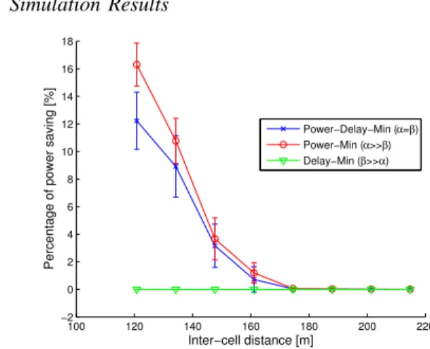
decision variables provided by the the LP relaxations. Thus, in a BB approach the number of integer variable determines the size of the search tree and influences the running time of the algorithm. B. Simulation Results 100 120 140 160 180 200 220 −2 0 2 4 6 8 10 12 14 16 18 Inter−cell distance [m]
Percentage of power saving [%]
Power−Delay−Min (α=β) Power−Min (α>>β) Delay−Min (β>>α)
Figure 3. Power Saving for the considered cases with respect to HPL model.
We start by examining how much power saving can be achieved for the three considered cases with respect to the HPL model while varying the inter-cell distance (D). The power saving is defined as: 1-the ratio between the total network power for the considered case and the total network power for the HPL model. Note that the total network power, defined in Equation 3 for the HPL model where all APs transmit at the first power level, equalsP9i=1Pi,1= 9 ∗ 10.296 = 92.664 W.
Figure 3 plots the percentage of power saving for the three considered cases as a function of the inter-cell distance. The Power-Min and the Power-Delay-Min cases show decreasing curves for D ranging between 120.8 m to 161.1 m. Further-more, they have no power saving gain for D ≥ 161.1 m. As expected, the figure shows that the Power-Min case has the highest percentage of power saving at 16% forD = 120.8 m, followed by the Power-Delay-Min case at 12% for the same D. The Delay-Min case has no power saving gain for all distances. In other words, in the Delay-Min case, we obtain a network configuration similar to the HPL model where all the APs transmit at the highest power level. This is because in this case we are interested in minimizing the sum of the user delays, therefore when all APs transmit at the highest level, users will experience lower delay in comparison with the case where some of the APs transmit at the second power level or are switched off.
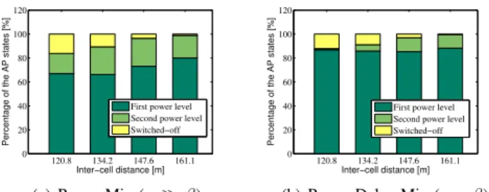
In order to examine the origin of power savings in the Power-Min and Power-Delay-Min cases, we plot Figures 4(a) and 4(b) that illustrate the percentage of the APs state for D equals 120.8 m to 161.1 m. We see that in the Power-Min case, we obtain percentages of APs transmitting at the second power level and switched off greater than that in the Power-Delay-Min case for the different values of D.
120.8 134.2 147.6 161.1 0 20 40 60 80 100 120 Inter−cell distance [m]
Percentage of the AP states [%]
First power level Second power level Switched−off (a) Power-Min (α ≫ β) 120.8 134.2 147.6 161.1 0 20 40 60 80 100 120 Inter−cell distance [m]
Percentage of the AP states [%]
First power level Second power level Switched−off
(b) Power-Delay-Min (α = β)
Figure 4. Percentage of the AP states for Power-Min and Power-Delay-Min
cases (a) (b).
Moreover, for the two cases, we see that whenD increases the percentage of switched off APs decreases, and the percentage of APs transmitting at the second power level increases. On the one hand, this explains the decreasing curves for the corresponding inter-cell distances in Figure 3. On the other hand, this behaviour is due, for low values of D, to the relatively high number of wireless signal layers; thus, the possibility to switch off the AP or to transmit at low power level is high. While whenD increases, the number of wireless signal layers decreases and thus the possibility to switch off the AP or to transmit at low power level decreases in order to ensure coverage for all users in the network.
100 120 140 160 180 200 220 6.5 7 7.5 8 8.5 9 9.5 10 10.5 11 11.5x 10 −5 Inter−cell distance [m]
Total network delay [sec] PB−UA/HPL
Power−Delay−Min (α=β) Power−Min (α>>β) Delay−Min (β>>α)
Figure 5. Total network delay for the considered cases and for PB-UA/HPL.
We now investigate the total network delay for the consid-ered cases compared to the PB-UA/HPL model while varying the inter-cell distance (D). As expected, for the comparison of the three cases, Figure 5 shows that the Delay-Min case has the lowest delay cost, followed by the Power-Delay-Min case and finally by the Power-Min case. Moreover, the figure shows that the curve corresponding to the PB-UA with the HPL model falls below the curves corresponding to the Power-Delay-Min and the Power-Min cases and performs close to the optimal solution of the Min case. This is because in the Delay-Min case, we obtain a network configuration where all APs transmit at the highest power level (similar to the HPL model) and thus the problem becomes a user association problem that aims to minimize the sum of network user delays. Further, we see that the delay cost of the Delay-Min has an increasing curve. This is because, for the same users distribution, whenD increases, the received power at the user side will decrease and thus the perceived rate at the current SNR will decrease which will cause the delay to increase. For the same reason, we see also that the Power-Delay-Min case has an increasing curve
but with lower slope at the first inter-cell distances. While, the Power-Min curve shows a decreasing curve forD between 120.8 m and 161.1 m and then it increases forD ≥ 161.1 m. This is because, forD between 120.8 m and 161.1 m, we tend to turn on more APs transmitting at either the highest power level or the second power level (Figure 4(a)) and thereby users will experience a lower delay. Note that all the curves tend to converge to the same point. This is expected because when D increases, the cell overlap decreases and thus the optimal solution for the three cases tend to turn on the APs, to achieve a point where all the APs transmit at the highest power level and therefore the problem will be a user association problem that minimizes the sum of user delays.
V. CONCLUSION
In this paper, we advocate a joint optimization for the double problem of power saving and user QoS satisfaction in a green wireless access network. Thus, we formulate a non-linear optimization problem that consists in finding a tradeoff between reducing the network power consumption and selecting the best user association that incurs the lowest sum of user transmission delays. We provide a linearization process of our problem that makes it computationally tractable for realistic scenarios. Different cases reflecting various decision preferences are studied by tuning the weights of the power and delay components of the network total cost. Compared to the most frequently deployed WLAN networks where APs transmit at a fixed transmit power level, results show that we obtain power savings of up to 16%. For future work, we plan to examine heuristics to solve the problem for dense scenarios.
REFERENCES
[1] The Benefits of Centralization in WLANs via the Cisco Unified Wireless
Network, 2006.
[2] Channels and Maximum Power Settings for Cisco Aironet Lightweight
Access Points, 2008.
[3] O. Eunsung and B. Krishnamachari. Energy savings through dynamic base station switching in cellular wireless access networks. In Proc.
IEEE GLOBECOM, USA, 2010.
[4] Andrea Goldsmith. Wireless Communications. Cambridge University Press, 2005.
[5] O. J. Grodzevich and O. Romanko. Normalization and other topics
in multi-objective optimization. In Workshop of the Fields MITACS
Industrial Problems, Canada, 2006.
[6] M. Heusse, F. Rousseau, G. Berger-Sabbatel, and A. Duda. Performance anomaly of 802.11b. In Proc. IEEE INFOCOM, USA, 2003. [7] K. Khawam, M. Ibrahim, J. Cohen, S. Lahoud, and S. Tohme. Individual
vs. global radio resource management in a hybrid broadband network. In Proc. IEEE ICC, Japan, 2011.
[8] J. Lorincz, A. Capone, and M. Bogarelli. Energy savings in wireless access networks through optimized network management. In Proc. IEEE
ISWPC, Italy, 2010.
[9] F. Moety, M. Ibrahim, S. Lahoud, and K. Khawam. Distributed heuristic algorithms for rat selection in wireless heterogeneous networks. In Proc.
IEEE WCNC, France, 2012.
[10] F. Richter, A. J. Fehske, and G. P. Fettweis. Energy efficiency aspects of base station deployment strategies for cellular networks. In Proc. IEEE
VTC Fall, USA, 2009.
[11] K. Son, H. Kim, Y. Yi, and B. Krishnamachari. Base station operation and user association mechanisms for energy-delay tradeoffs in green cellular networks. IEEE JSAC, 2011.
[12] S. Tombaz, M. Usman, and J. Zander. Energy efficiency improvements through heterogeneous networks in diverse traffic distribution scenarios. In Proc. IEEE ICST, China, 2011.